0.5in

Cross-correlation (C²) Imaging for Waveguide Characterization

©   Copyright by 2012

Approved by

First Reader   Siddharth Ramachandran, Ph.D. Associate Professor of Electrical Engineering
Second Reader   Jerome Mertz, Ph.D. Professor of Biomedical Engineering
Third Reader   M. Selim Ünlü, Ph.D. Professor of Biomedical and Electrical Engineering

Chapter 1 Introduction

In optical applications, the demand for reliable waveguide characterization methods comes from the development of several fiber-based optical technologies. First, the network traffic in optical fiber communication systems demands further increase in optical channels to overcome the limitations of currently deployed wave-division multiplexing (WDM) systems, such as the bandwidth of optical amplifiers and input power.

Mode-division multiplexing (MDM) pioneered in Ref. [Berdagué and Facq, 1982] and recently developed in Refs.[Hanzawa et al., 2011, Ryf et al., 2011, Salsi et al., 2011] is one possible solution of the network-capacity problem. MDM systems employing several fiber modes for transmission of information require real-time monitoring of modal power decomposition.

Several approaches have been suggested to realize the monitoring, such as the far-field imaging of the output facet of multimoded fibers [Rittich, 1985], and a method using ultrafast sources and specially designed probe fibers to temporally resolve the launched power [Golowich et al., 2004]. A promising alternative for modal power monitoring in real-time is provided by the tilted-fiber Bragg gratings. The gratings couple guided modes to radiation modes encoding, among other characteristics, the modal power distribution in the probed systems [Wagener et al., 1997, Westbrook et al., 2000, Feder et al., 2003, Yang et al., 2005, Yan et al., 2012].

High-performance, high-power fiber-lasers [Richardson et al., 2010] is another area in which waveguide characterization is of outmost importance. The design of novel fiber-platforms capable of achieving excellent output beam-qualities requires the propagation of only one mode in fibers that are not strictly single-moded [Dong et al., 2009, Ramachandran et al., 2006, Galvanauskas et al., 2008, Stutzki et al., 2011, Koplow et al., 2000]. A usual measure of the laser-beam quality in these systems is the so-called M²-parameter [Siegman, 1990a, Siegman, 1990b]. However, being essentially an integral characteristic, it gives a very rough estimate of higher-order mode content [Wielandy, 2007].

A recently reported characterization technique – S² imaging [Nicholson et al., 2008, Nicholson et al., 2009] – enables the direct measurement of modal content of multimoded waveguides by recording spatially resolved output of the fiber in frequency domain. Historically, this approach appeared from the early studies of mode dispersion of higher-order modes [Menashe et al., 2001] and multi-path interference [Ramachandran et al., 2003, Ramachandran et al., 2005, Ramachandran, 2005]. In S²-imaging method, one of the modes, usually the fundamental one, is used as a “reference” mode for the analysis of the interference signal, which is a fundamental impediment of the approach. In particular, in this case, a reasonable estimate of the relative power levels of the modes may be obtained only when the “reference” mode has the largest power in the propagating beam. Moreover, the presence of multiple interferences of every mode with all other modes complicates the analysis of the recorded signal and makes the power reconstruction unreliable. As a result, the method fails to characterize the generic case of multiple modes having similar power levels. Yet another difficulty is related to the inherent insensitivity of the method to the polarization properties of the modes, which introduces uncontrollable approximations in the interpretation of the results, in the general case of elliptically polarized states.

An alternative approach of optical low-coherence interferometry does not suffer from the limitations of S²-imaging, since it employs the external reference beam with well-defined characteristics, which interferes with all the modes of the test waveguide [Nandi et al., 2009, Ma et al., 2009]. This technique does not require any prior knowledge of group-delay or dispersive characteristics of the reference mode. In contrast to S² imaging, all the modes having arbitrary relative power levels and polarization properties can be measured independently of one another.

In this work, I have developed and realized this idea. In particular, I have worked out the mathematical formalism forming the basis of the method and demonstrated that interferometric signal contains complete information about waveguide modes, including modal decomposition, intensity and phase distributions of all the modes, and also their polarization properties. The formalism was applied for characterization of several optical waveguides with distinct properties and successfully demonstrated all the declared capabilities.

The core of my Thesis begins in Chapter 2 with general discussion of the mathematical formalism of cross-correlation imaging. Application of the method to characterization of several optical waveguides is demonstrated in Chapter 3. The summary of my experimental and theoretical work is presented in Chapter 4.

Chapter 2 Mathematical formalism of C²-imaging

In this Chapter, I discuss the mathematical formalism of C²-imaging [Barankov and Ramachandran, 2012], which forms the basis of the experimental method applied in Chapter 3 for characterization of several optical waveguides. In Section 2.1, I introduce the general framework of waveguide interferometry necessary for basic applications of the method. Then, in Section 2.2, I present a modification of the method suitable for studies of polarization properties of waveguide modes. Finally, in Section 2.3, I describe phase-sensitive modification of the method.

2.1 General description of C²-imaging

In this section, I provide the basic description of the mathematical formalism of C²-imaging method. Some elements of the formalism were already presented in Ref. [Schimpf et al., 2011]; here, I expand and further develop this early discussion.

In multimoded optical waveguides, a beam of light propagates as a superposition of discrete modes characterized by different propagation constants and various intensity patterns of the modes, depending on the boundary conditions. Direct imaging of the beam provides the intensity distribution and also the output power averaged over superposition of all the modes. The goal of this section is to demonstrate a novel interferometric approach that allows characterization of modal powers and intensity distribution of every waveguide mode contributing to the superposition state.

The basic idea of the method is to study the interference of the beam radiated from an optical waveguide with an external reference beam and detect different waveguide modes in the time-domain by changing the relative optical paths of the two beams.

2.1.1 Interferometry of optical beams

In this work, we employ the standard Mach-Zehnder interferometer configuration shown in Figure 2$\cdot$1 to study the interference of the reference and the test beam radiated from the signal waveguide. The beam of light from an LED source is divided into two beams at the beam-splitter and then, after propagating in the reference and test waveguides, recombined at the beam combiner. The beam of light, radiated from a single-moded reference fiber, is collimated, while the signal beam of the test fiber is focused at the camera. The camera records a stack of images at different positions of the delay stage.

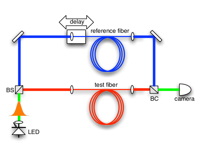
Figure 2$\cdot$1: C²-imaging setup: LED – light-emitting diode, BS – beam-splitter, BC – beam combiner, Delay – delay stage.

The electric field at the image plane of the camera is a superposition of two fields

$${\bf E}({\bf r},t)={\bf E}_{r}({\bf r},t)+{\bf E}_{s}({\bf r},t+\tau),$$ (2.1)

where ${\bf E}_{r}({\bf r},t)$ and ${\bf E}_{s}({\bf r},t)$ are the electric fields of the reference and signal beams, correspondingly.

The signal beam is delayed by time

$$\tau=d/c$$ (2.2)

with respect to the reference beam, where $d$ is the free-space difference between the two optical paths, and $c$ is the speed of light in vacuum. The time delay is introduced by the delay stage shown in Fig. 2$\cdot$1.

The camera records the intensity of light averaged over the exposure time, which allows to employ the two equivalent representations of the electric fields in time and frequency domains, ${\bf E}({\bf r},\omega)=\int dt\,e^{i\omega t}{\bf E}({\bf r},t)$, according to the well-known identity (Parseval’s theorem):

$$I({\bf r},\tau)=\int\limits_{-\Delta T/2}^{+\Delta T/2}\mbox{d}t|{\bf E}({\bf r},t)|^{2}=\int\limits_{-\infty}^{+\infty}\frac{\mbox{d}\omega}{2\pi}\,|\mathbf{E}({\bf r},\omega)|^{2},$$ (2.3)

where ${\bf r}=(x,y)$ defines the position of the camera pixel in the imaging plane, and $\Delta T$ is the exposure time of the camera, assumed to be much larger than the characteristic period of the electric field oscillations.

Upon substitution of the electric field (2.1) into Eq. (2.3), we arrive at the expression for the average intensity that contains the background intensities of the reference and the signal beams $I_{0}$, independent of the time-delay $\tau$, and also the interferometric intensity $I_{int}$

$$I({\bf r},\tau)=I_{0}({\bf r})+I_{int}({\bf r},\tau),$$ (2.4)

with two terms written explicitly as

$$I_{0}({\bf r})=\int_{-\infty}^{+\infty}\frac{d\omega}{2\pi}\,\left(|{\bf E}_{r}({\bf r},\omega)|^{2}+|{\bf E}_{s}({\bf r},\omega)|^{2}\right),$$ (2.5)

$$I_{int}({\bf r},\tau) = 2\mathbf{Re}\,\int_{-\infty}^{\infty}dt\,{\bf E}^{*}_{r}({\bf r},t){\bf E}_{s}({\bf r},t+\tau)$$ (2.6)

$$= 2{\rm\bf Re}\,\int_{-\infty}^{+\infty}\frac{d\omega}{2\pi}\,{\bf E}_{r}^{*}({\bf r},\omega){\bf E}_{s}({\bf r},\omega)e^{-i\omega\tau},$$

According to these equations, the interferometric signal $I_{int}\sim{\bf E}_{r}^{*}{\bf E}_{s}\sim e^{i\varphi_{rs}-i\omega\tau}$ is sensitive to the optical path difference $\varphi_{rs}=\varphi_{r}-\varphi_{s}$ and also the time-delay $\tau$.

2.1.2 Analysis of interferometric signal

The electric fields of the reference and signal beams in Eqs. (2.5) and (2.6) are given by

$${\bf E}_{r}({\bf r},\omega) = {\bf e}_{r}({\bf r},\omega)A_{r}(\omega)e^{i\varphi_{r}},$$

$${\bf E}_{s}({\bf r},\omega) = \sum_{m}\alpha_{m}{\bf e}_{m}({\bf r},\omega)A_{m}(\omega)e^{i\varphi_{m}},$$ (2.7)

where the electric field ${\bf E}_{s}$ is a superposition of waveguide modes ${\bf E}_{m}$ with real modal amplitudes $\alpha_{m}$. The power of the $m$-th mode is given by

$$p_{m}=\alpha_{m}^{2}.$$ (2.8)

The spectral properties of the reference beam and waveguide modes are encoded in the corresponding functions $A_{r}\left(\omega\right)$ and $A_{m}\left(\omega\right)$.

Every mode of the signal beam and the reference beam is characterized by the intensity distribution:

$$I_{ref}({\bf r},\omega)=|{\bf e}_{r}({\bf r},\omega)|^{2},\,I_{m}({\bf r},\omega)=|{\bf e}_{m}({\bf r},\omega)|^{2}.$$ (2.9)

The intensity distribution $I_{ref}({\bf r},\omega)$ of the reference beam is imaged directly by blocking the signal path of the interferometer. A similar direct measurement of the signal beam, done by blocking the reference path, produces only the total intensity distribution $I_{tot}=\sum_{m}I_{m}$ of all the modes propagating in the signal beam, and, thus, does not provide access to the intensities of individual modes.

The goal of this section is to demonstrate that C²-imaging allows to separately measure the intensity distribution and relative power level of every mode of the signal beam, employing the property of the modes to experience different phase shifts upon propagation in a waveguide.

Specifically, the $m$-th mode, after propagation in the test fiber of length $L$, acquires the phase

$$\varphi_{m}=\beta_{m}\left(\omega\right)L,$$ (2.10)

where $\beta_{m}\left(\omega\right)$ is the propagation constant of the mode.

The phase of the reference field, propagating in a single-mode reference fiber of length $L_{r}$, is given by

$$\varphi_{r}=\beta_{r}\left(\omega\right)L_{r},$$ (2.11)

where $\beta_{r}(\omega)$ is the propagation constant, and $L_{r}$ is the length of the reference fiber.

The transverse phase-profile of the reference beam is assumed flat at the imaging plane, which is satisfied by the collimation of the beam and also ensuring that the imaging plane coincides with the neck of the collimated beam. Regarding the signal beam, the near-field image of the output facet of the signal fiber is recorded, by focusing the beam at the imaging plane.

By substituting the electric field of Eq. (2.1.2) into Eq. (2.6), we arrive at the expression for the intensity $I_{int}({\bf r},\tau)$, which accounts for the interference between the reference field and the individual modes:

$$I_{int}({\bf r},\tau)=2\textbf{Re}\sum_{m}\int\limits_{-\infty}^{+\infty}\frac{\mbox{d}\omega}{2\pi}\,{\bf e}_{r}^{*}({\bf r},\omega)A_{r}^{*}(\omega)\alpha_{m}{\bf e}_{m}({\bf r},\omega)A_{m}(\omega)e^{i(\varphi_{m}-\varphi_{r}-\omega\tau)}.$$ (2.12)

The analysis of this expression simplifies if one makes several reasonable assumptions. In particular, since we are mainly interested in optical measurements, typically performed with relatively narrow spectral widths around the central frequency of the source, it is usually safe to assume that the electric fields do not significantly vary in this spectral window

$$\mathbf{e}\left({\bf r},\omega\right)\approx\mathbf{e}\left({\bf r},\omega_{0}\right),$$ (2.13)

where $\omega_{0}$ is the central frequency of the light source.

Then Eq. (2.12) simplifies:

$$I_{int}({\bf r},\tau)=2\textbf{Re}\sum_{m}\alpha_{m}{\bf e}_{r}^{*}({\bf r},\omega_{0}){\bf e}_{m}({\bf r},\omega_{0})G_{rm}\left(\tau+\tau_{rm}\right)e^{-i\theta_{rm}},$$ (2.14)

where I introduced the joint coherence function

$$G_{rm}\left(t\right) = \int\frac{d\Omega}{2\pi}\,e^{-i\Omega t}\,S_{rm}\left(\Omega\right),$$

$$S_{rm}(\Omega) = A^{*}_{r}(\Omega)A_{m}(\Omega)e^{-i\varphi_{rm}\left(\Omega\right)},$$ (2.15)

and defined the spectral functions with respect to a shifted frequency

$$\Omega=\omega-\omega_{0}.$$ (2.16)

The joint coherence function depends on the differential group-delay of every mode propagating in the signal beam with respect to the reference beam

$$\tau_{mr}=L/v_{gr,m}-L_{r}/v_{gr,r}.$$ (2.17)

The group-velocity dispersion mismatch between the two beams is accounted for by the frequency-dependent phase

$$\varphi_{mr}=\sum_{k\geq 2}(\beta_{m}^{(k)}L-\beta_{r}^{(k)}L_{r})\Omega^{k}/k!,$$ (2.18)

where $\beta^{(k)}$ stand for the Taylor-coefficients of the mode-propagation constant $\beta$ calculated at the central frequency $\omega_{0}$ of the source.

The dominant contribution to the time-delay variation of the interferometric intensity comes from the zero-order optical path mismatch of the beams defined at the central frequency of the source

$$\theta_{mr}=\beta_{m}^{(0)}L-\beta_{r}^{(0)}L_{r}-\omega_{0}\tau.$$ (2.19)

The joint coherence function describes the impact of the frequency-dependent mode-propagation constant and the spectral properties of the fields on the interferometric signal. In particular, the group-delay $\tau_{mr}$ defines the position of $m$-th mode in the interferometric trace recorded by the camera at a given transverse position in the imaging plane, and the shape of the trace is determined by the joint spectral function of the reference and the signal beams $S_{rm}$. In cases when waveguide modes do not undergo spectral filtering (e.g. due to a long period grating embedded in the waveguide), the spectral functions of the two beams are identical, $A=A_{m}=A_{r}$, and the joint spectral function is given by $S_{rm}=S_{0}e^{-i\varphi_{rm}}$, where $S_{0}=|A|^{2}$ is the spectrum of the light source.

The general expressions (2.14) and (2.1.2), describing interference of the signal and the reference beams, form the basis of further theoretical analysis and experiments.

2.1.3 Determination of mode dispersion and relative group delays

The structure of the coherence function defines dispersive properties of the modes. Specifically, the complex-valued joint coherence function may be represented as a product of the real-valued amplitude and the phase factor:

$$G_{mr}(\tau)={\cal G}_{mr}(\tau)e^{-i\psi_{mr}(\tau)},$$ (2.20)

which certainly depend on the detailed structure of the source spectrum. In general, however, these are slowly varying functions on the time scale of the electric field oscillations $2\pi/\omega_{0}$.

An important property of the joint coherence function is the normalization, which is independent of the dispersive properties of the modes. Indeed, it is determined only by the spectral properties, as it follows from the identities

$$\int\limits_{-\infty}^{\infty}d\tau\,|G_{mr}(\tau)|^{2}=\int\limits_{-\infty}^{\infty}d\tau\,{\cal G}^{2}_{mr}(\tau)=\int\limits_{-\infty}^{\infty}\frac{d\Omega}{2\pi}\,\left|A_{m}(\Omega)\right|^{2}\left|A_{r}(\Omega)\right|^{2}.$$ (2.21)

Normalization condition also indicates that the amplitude of the joint coherence function ${\cal G}_{mr}(t)$ has finite extent $\Lambda_{m}$ in the time domain defined as

$$t\in\Lambda_{m}:|t|\leq\delta t_{m}\sim 1/\Delta\omega,$$ (2.22)

which is dictated by the smallest spectral width of the reference and the signal beams $\Delta\omega$. The time-extent $\delta t_{m}$ is usually mode-dependent, due to the dispersion effects.

The separation of time-scales, $\delta t_{m}\gg 1/\omega_{0}$ suggests time-averaging of the square of the interference term (2.14) on the time-scale $1/\omega_{0}\ll\Delta t\ll\delta t_{m}$. After the averaging, we obtain

$${\cal P}_{r}({\bf r},\tau)=\frac{1}{2\Delta t}\int\limits_{\tau-\Delta t/2}^{\tau+\Delta t/2}dt\,I_{int}^{2}({\bf r},t)/I_{ref}({\bf r})=\sum_{m}p_{m}|\hat{e}^{*}_{r}\hat{e}_{m}|^{2}{\cal G}_{mr}^{2}(\tau-\tau_{mr})I_{m}({\bf r}),$$ (2.23)

where $p_{m}$ is the modal power, $\hat{e}_{r}$ and $\hat{e}_{m}$ are the polarization unit vectors of the reference and signal beams, and

$$I_{ref}({\bf r})=|{\bf e}_{r}({\bf r},\omega_{0})|^{2},\,I_{m}({\bf r})=|{\bf e}_{m}({\bf r},\omega_{0})|^{2}$$ (2.24)

are the intensity distributions of the reference and signal beam at the central frequency of the source.

By measuring the interference signal for a full set of polarization states of the reference beam, one finds the intensity as a function of the time-delay:

$${\cal P}({\bf r},\tau)=\sum_{r}{\cal P}_{r}({\bf r},\tau)=\sum_{m}p_{m}{\cal G}_{mr}^{2}(\tau-\tau_{mr})I_{m}({\bf r}).$$ (2.25)

This expression indicates a strategy for separating waveguide modes in the time-domain. In particular, provided the differential group delay of the two nearby modes is larger than the characteristic extent of the coherence function, i.e. $\tau_{m,m+1}\gtrsim\delta t$, the interference peaks corresponding to these modes are well-separated in the time-domain. In this case, the intensity ${\cal P}({\bf r},\tau)$ at every position ${\bf r}$ in the imaging plane exhibits a series of well-separated peaks located at $\tau=\tau_{mr}$, having the shapes determined by the spectral functions of the modes.

Therefore, by employing an appropriate fitting procedure of the joint coherence function to the measured interferometric signal, one finds the relative group delays and determines dispersive properties of the modes. In cases when the dispersion of the reference beam is unknown, one can measure the interferometric signal at several different lengths of the reference waveguide, and then use the resulting set of equations to determine dispersion characteristics of all the modes, including the reference mode.

2.1.4 Reconstruction of modal weights and intensity distributions

The structure of the joint coherence function allows determination of the modal weights without detailed knowledge of the source spectrum. Indeed, the modal intensity distribution and power of every mode can be found by, first, integrating Eq. (2.25) over the extent $\Lambda_{m}$ and then integrating over the imaging plane:

$$I_{m}({\bf r}) = \int\limits_{\Lambda_{m}}d\tau\,{\cal P}({\bf r},\tau),$$

$$p_{m} = \int\limits_{\Lambda_{m}}d\tau\int d{\bf r}\,{\cal P}({\bf r},\tau),$$ (2.26)

where it is assumed that the modal intensity and spectral function (same for all modes) are normalized to unity, i.e.

$$\int\frac{d\Omega}{2\pi}|S_{mr}(\Omega)|^{2}=1,\,\int d{\bf r}\,I_{m}({\bf r})=1.$$ (2.27)

The relative powers $p_{m}$ of all waveguide modes can be reliably extracted from the interference signal only when the coherence peaks do not significantly overlap. When some peaks do overlap, e.g. due to their relatively small differential group delay, the outlined procedure may still be used. However, in this case it will provide the relative power of the corresponding group of overlapping peaks. The formalism presented above can not discriminate the degenerate modes. Below, I introduce a polarization-sensitive modification of the method that allows the reconstruction of degenerate modes, using their polarization properties. One example of such reconstruction is demonstrated in Chapter 3. Other modifications, accounting for mode-dependent spectral properties, are also possible.

2.1.5 Gaussian model

The general description of the beam interferometry presented in the previous section is illustrated in this part, assuming same spectral characteristics of the signal and reference beams, $A=A_{m}=A_{r}$, and using a gaussian model of the light source

$$S(\Omega)=S_{0}\exp{\left[-(\Omega/\Delta\Omega)^{2}\right]},\,\Omega=\omega-\omega_{0},$$ (2.28)

centered at $\omega_{0}$ with the spectral width $\Delta\Omega$. To simplify the calculation, I consider only the effects of group-velocity dispersion

$$\varphi_{mr}\approx\left(\beta_{m}^{(2)}L-\beta_{r}^{(2)}L_{r}\right)\Omega^{2}/2.$$ (2.29)

Under these conditions, the integral in Eq.(2.1.2) can be analytically calculated, which leads to the following expression for the interferometric intensity

$${\cal P}({\bf r},\tau)=\sum_{m}p_{m}I_{m}({\bf r})\frac{\Delta\Omega}{\sqrt{2\pi\left(1+d_{mr}^{2}\right)}}\exp\left[-\frac{\left(\tau-\tau_{mr}\right)^{2}\Delta\Omega^{2}}{2\left(1+d_{mr}^{2}\right)}\right]$$ (2.30)

where the dispersion effects are included into the dimensionless parameter

$$d_{mr}=(\beta_{m}^{(2)}L-\beta_{r}^{(2)}L_{r})\Delta\Omega^{2}/2,$$ (2.31)

and the modal intensities $I_{m}({\bf r})$ are normalized.

Eq. (2.30) indicates that relative height of the interference peaks strongly depends on the dispersion effects: for larger dispersion, the time extent of the peak increases while its height correspondingly decreases, so that the normalization of the coherence function is preserved. This observation is generally true for any spectrum properties of the reference and signal beams and suggest the use of the integral characteristics instead of the peak value for measurements of the modal powers.

2.1.6 Dispersion compensation

The temporal extent of the interference peaks corresponding to different modes defines the temporal resolution of C²-imaging. Most clearly this limitation appears in the analysis of the gaussian model, where the temporal full-width at half-maximum of the interference peak

$$\Delta\tau_{FWHM}=\sqrt{8\ln 2}\sqrt{1+d^{2}_{mr}}/\Delta\Omega.$$ (2.32)

is determined by the spectral width $\Delta\Omega$ of the source and group-velocity dispersion mismatch between the two beams $d_{mr}$. Obviously, this expression provides an estimate for the temporal resolution of the method, assuming that a pair of the modes with small relative group delay have similar group-velocity dispersions.

As it follows from Eq. (2.32), temporal resolution approaches the limiting value

$$\Delta\tau_{FWHM}=\sqrt{8\ln 2}/\Delta\Omega,$$ (2.33)

when the lengths of the reference and the test fibers are matched, i.e.

$$L_{opt}=L\,\beta_{m}^{(2)}/\beta_{r}^{(2)},$$ (2.34)

so that the group-velocity dispersion is fully compensated.

For an arbitrary non-gaussian spectrum, the condition of the dispersion-compensation remains the same. Indeed, the dispersion effects are accounted for by the frequency-dependent phase

$$\varphi_{mr}=\sum_{k\geq 2}\left(\beta_{m}^{(k)}L-\beta_{r}^{(k)}L_{r}\right)\Omega^{k}/k!,$$ (2.35)

The structure of the phase shows that the impact of dispersion is minimized when the length of the reference waveguide satisfies

$$L_{opt}=L\,\beta_{m}^{(k)}/\beta_{r}^{(k)},$$ (2.36)

where $k$ is the order of the first non-vanishing dispersion term. The dispersion effects usually become noticeable already at $k=2$, and, as expected, this condition then reproduces Eq. (2.34). It’s worth noting that conditions (2.34), and (2.36) can be satisfied only when the ratios of the corresponding dispersive coefficients $\beta_{m}^{(k)}/\beta_{r}^{(k)}>0$.

In practice, it is possible to compensate the dispersion effects for a single mode or a group of modes with similar dispersion characteristics. The residual dispersion of other non-compensated modes results in their temporal broadening.

Certainly, the limit of the temporal resolution (2.33) can only be achieved for purely parabolic dispersion. In more general situations, higher-order dispersive terms may become important. For example, when the group-velocity dispersion is fully compensated, the third-order phase term contributes a correction to the spectrally limited temporal resolution of the order

$$d^{(3)}_{mr}\simeq L\Delta\Omega^{3}\left(\beta_{r}^{(2)}\beta_{m}^{(3)}-\beta_{r}^{(3)}\beta_{m}^{(2)}\right)/\left(6\beta_{r}^{(2)}\right),$$ (2.37)

which depends on the spectral properties of the system and the length of the test waveguide. Under usual conditions, this correction is expected to be small.

2.2 Polarization-sensitive imaging

In this section, I describe how C²-imaging can be used to reconstruct polarization state of the modes propagating in few-moded optical waveguides [Barankov et al., 2012b]. Specifically, I show that the measurement of the cross-correlation signal for six different polarization states of the reference beam allows full characterization of the polarization state of every mode of the test beam in terms of the spatially-dependent Stokes parameters. A specific implementation and application of this method is demonstrated in Chapter 3.

2.2.1 Polarization states

In spinor notations, every polarization state of $m$-th mode can be expressed as a vector with two components

$$\hat{e}_{m}=\left(\begin{array}[]{c}E_{x}\\ E_{y}\end{array}\right)=e^{i\alpha_{x}}\left(\begin{array}[]{c}|E_{x}|\\ |E_{y}|e^{i\varphi}\end{array}\right),$$ (2.38)

where $\varphi=\alpha_{y}-\alpha_{x}$ is the relative phase of the complex amplitudes $E_{x}=|E_{x}|e^{i\alpha_{x}}$ and $E_{y}=|E_{y}|e^{i\alpha_{y}}$. The absolute phase, without loss of generality, can be neglected.

The complete characterization of the polarization state requires identification of the following three pairs of orthonormal basis states. The first pair is formed by the states linearly polarized along $x$- and $y$-axis:

$$|H\rangle=\left(\begin{array}[]{c}1\\ 0\end{array}\right),\quad|V\rangle=\left(\begin{array}[]{c}0\\ 1\end{array}\right).$$ (2.39)

Another pair is obtained by rotating the basis by $\pi/4$ radians:

$$|+\rangle=\frac{1}{\sqrt{2}}\left(\begin{array}[]{c}1\\ 1\end{array}\right),\quad|-\rangle=\frac{1}{\sqrt{2}}\left(\begin{array}[]{c}1\\ -1\end{array}\right).$$ (2.40)

The last pair is given by the left and right circularly polarized states:

$$|L\rangle=\frac{1}{\sqrt{2}}\left(\begin{array}[]{c}1\\ -i\end{array}\right),\quad|R\rangle=\frac{1}{\sqrt{2}}\left(\begin{array}[]{c}1\\ i\end{array}\right).$$ (2.41)

Experimentally, projection onto these six states can be realized using combinations of a linear polarizer, half-wave and also quarter-wave plate, characterized by the following matrices

$$T_{LP}(\theta) = \left[\begin{array}[]{cc}\cos^{2}\theta&\sin\theta\cos\theta\\ \sin\theta\cos\theta&\sin^{2}\theta\end{array}\right],$$ (2.44)

$$T_{HWP}(\theta) = \left[\begin{array}[]{cc}-\cos 2\theta&-\sin 2\theta\\ -\sin 2\theta&\cos 2\theta\end{array}\right],$$ (2.47)

$$T_{QWP}(\theta) = \left[\begin{array}[]{cc}i\cos^{2}\theta+\sin^{2}\theta&(i-1)\sin\theta\cos\theta\\ (i-1)\sin\theta\cos\theta&i\sin^{2}\theta+\cos^{2}\theta\end{array}\right],$$ (2.50)

where $\theta$ determines the angle of the fast axis of the corresponding polarizing element.

A specific implementation of the projections onto these states is demonstrated in Chapter 3.

2.2.2 Stokes parameters

An arbitrary state of polarized or unpolarized light is characterized by the Stokes vector ${\bf S}=(S_{0},S_{1},S_{2},S_{3})$ with the following components:

$$S_{0} = \langle|E_{x}|^{2}\rangle+\langle|E_{y}|^{2}\rangle,$$

$$S_{1} = \langle|E_{x}|^{2}\rangle-\langle|E_{y}|^{2}\rangle,$$

$$S_{2} = 2\langle|E_{x}E_{y}|\cos\varphi\rangle,$$

$$S_{3} = 2\langle|E_{x}E_{y}|\sin\varphi\rangle,$$ (2.51)

where averaging $\langle...\rangle$ is taken with respect to an ensemble of measurements. When $E_{x}$, $E_{y}$ and $\varphi$ do not vary within the ensemble, the light is completely polarized.

2.2.3 Polarization distribution of waveguide modes

In C²-imaging, the intensity distribution function is proportional to the scalar product of the polarizations of the reference beam $\hat{e}_{r}$ and the $m$-th mode $\hat{e}_{m}({\bf r})=(E_{x}({\bf r}),E_{y}({\bf r}))^{T}$ (transposed vector) of the signal beam:

$${\cal P}_{rm}({\bf r},\tau)=p_{m}I_{m}({\bf r})\left|\hat{e}^{*}_{r}\hat{e}_{m}({\bf r})\right|^{2}{\cal G}^{2}_{rm}(\tau-\tau_{mr}),$$ (2.52)

The intensity distribution $I_{m}({\bf r})$ is obtained from this expression by summation over a complete set of reference states (e.g. $|H\rangle$ and $|V\rangle$) and then integrating over the temporal extent of the mode $\Lambda_{m}$, as described earlier in this Chapter.

The polarization state of every mode, corresponding to a peak value of the coherence function ${\cal G}(\tau-\tau_{mr})$ at $\tau=\tau_{mr}$, can be reconstructed from the measurement of six different polarization states of the reference beam $\hat{e}_{r}$. The number of measurements is reduced to four when one accounts for the symmetry of the basis states.

It is convenient to introduce polarization distribution function

$${\cal U}_{rm}({\bf r})=\int_{\Lambda_{m}}d\tau\,{\cal P}_{rm}({\bf r},\tau)/\left(p_{m}I_{m}({\bf r})\right)=\left|\hat{e}^{*}_{r}\hat{e}_{m}({\bf r})\right|^{2},$$ (2.53)

sensitive to the overlap of the reference polarization and spatially dependent mode-polarization.

Straightforward calculations carried out for six spatially uniform polarization states of the reference beam lead to the following set of equations:

$${\cal U}_{H} = |E_{x}|^{2},\quad{\cal U}_{V}=|E_{y}|^{2},$$

$${\cal U}_{+} = \frac{1}{2}\left(|E_{x}|^{2}+|E_{y}|^{2}\right)+|E_{x}E_{y}|\cos\varphi,$$

$${\cal U}_{-} = \frac{1}{2}\left(|E_{x}|^{2}+|E_{y}|^{2}\right)-|E_{x}E_{y}|\cos\varphi,$$

$${\cal U}_{L} = \frac{1}{2}\left(|E_{x}|^{2}+|E_{y}|^{2}\right)-|E_{x}E_{y}|\sin\varphi,$$

$${\cal U}_{R} = \frac{1}{2}\left(|E_{x}|^{2}+|E_{y}|^{2}\right)+|E_{x}E_{y}|\sin\varphi,$$ (2.54)

with the obvious symmetry identities ${\cal U}_{0}={\cal U}_{H}+{\cal U}_{V}={\cal U}_{+}+{\cal U}_{-}={\cal U}_{L}+{\cal U}_{R}$.

The spatial distribution of the Stokes vector of the $m$-th mode is directly obtained from these relations, by averaging over the ensemble of measurements:

$$S_{0}({\bf r}) = \langle{\cal U}_{H}\rangle+\langle{\cal U}_{V}\rangle=\langle{\cal U}_{0}\rangle,$$

$$S_{1}({\bf r}) = \langle{\cal U}_{H}\rangle-\langle{\cal U}_{V}\rangle=2\langle{\cal U}_{H}\rangle-\langle{\cal U}_{0}\rangle,$$

$$S_{2}({\bf r}) = \langle{\cal U}_{+}\rangle-\langle{\cal U}_{-}\rangle=2\langle{\cal U}_{+}\rangle-\langle{\cal U}_{0}\rangle,$$

$$S_{3}({\bf r}) = \langle{\cal U}_{R}\rangle-\langle{\cal U}_{L}\rangle=2\langle{\cal U}_{R}\rangle-\langle{\cal U}_{0}\rangle$$ (2.55)

In the case of a polarized light, the electric fields do not fluctuate within the measurement ensemble, and the formalism simplifies due to the identity $S_{0}^{2}=S_{1}^{2}+S_{2}^{2}+S_{3}^{2}$ limiting the polarization vector to the surface of the Poincaré sphere.

This formalism has been used to obtain the spatial distribution of the Stokes vector in the case of vortex states, as discussed in Chapter 3.

2.3 Phase-sensitive imaging

Spatial phase $\varphi_{m}({\bf r})$ is one of the key characteristics of waveguide modes, illustrating the complex nature of electric field:

$${\bf e}_{m}({\bf r},\omega_{0})=\sqrt{I_{m}({\bf r})}\exp\left[-i\varphi_{m}({\bf r})\right]\hat{e}_{m}({\bf r}),$$ (2.56)

Although in some trivial cases an irrelevant factor, the phase is essential for understanding the vortex modes recently obtained in optical waveguides.

In this section, I describe how one can use phase-sensitive C²-imaging for reconstruction of the spatial phase profile of waveguide modes [Barankov et al., 2012a]. In particular, the intensity distribution of the interferometric signal contains overlap of the reference and $m$-th waveguide modes:

$$I_{int}({\bf r},\tau)=2\textbf{Re}\sum_{m}\alpha_{m}{\bf e}_{r}^{*}({\bf r},\omega_{0}){\bf e}_{m}({\bf r},\omega_{0})G_{rm}\left(\tau-\tau_{mr}\right)e^{-i\theta_{rm}},$$ (2.57)

The intensity distributions of the reference beam and the $m$-th mode, as well as the polarization distributions can be obtained by the methods described earlier in this Chapter. It becomes possible, therefore, as it follows from Eq. (2.57), to introduce the phase function that accounts only for the impact of the temporal dependence of the coherence function and the spatially dependent phase of the $m$-mode:

$${\cal I}_{rm}({\bf r},\tau)={\cal G}_{rm}(\tau)\cos\left[\varphi_{m}({\bf r})-\omega_{0}\tau+\psi_{rm}(\tau)+\theta_{rm}(\tau_{mr})\right],$$ (2.58)

where, to simplify the notations, time variable was redefined: $\tau-\tau_{mr}\to\tau$. Here, $\psi_{rm}(\tau)$ and ${\cal G}_{rm}(\tau)$ are the phase and magnitude of the coherence function $G_{rm}(\tau)$, varying on the time-scale significantly larger than the period $2\pi/\omega_{0}$ of the electric field.

As it follows from Eq. (2.58), one can use the following strategy to extract the spatial phase $\varphi_{m}({\bf r})$ from the phase function (2.58). For a given position ${\bf r}_{*}$, we identify moments of time $\tau_{max}$ and $\tau_{0}$, such that $\tau_{max}-\tau_{0}\leq\pi/(2\omega_{0})$ and

$${\cal I}_{rm}({\bf r}_{*},\tau_{max})={\cal G}_{rm}(\tau_{max}),\quad{\cal I}_{rm}({\bf r}_{*},\tau_{0})=0:\,\tau_{max}-\tau_{0}\leq\pi/(2\omega_{0}).$$ (2.59)

As a result, one finds two complimentary functions

$${\cal I}_{rm}({\bf r},\tau_{max}) = {\cal G}_{rm}(\tau_{max})\cos\left[\varphi({\bf r})-\varphi({\bf r}_{*})\right],$$

$${\cal I}_{rm}({\bf r},\tau_{0}) = {\cal G}_{rm}(\tau_{0})\sin\left[\varphi({\bf r})-\varphi({\bf r}_{*})\right],$$ (2.60)

which allow reconstruction of the spatial phase

$$\varphi({\bf r})-\varphi({\bf r}_{*})=-i\,\ln\left[{\cal I}_{rm}({\bf r},\tau_{max})/{\cal G}_{rm}(\tau_{max})+i\,{\cal I}_{rm}({\bf r},\tau_{0})/{\cal G}_{rm}(\tau_{0})\right].$$ (2.61)

This approach has been used for reconstruction of spatial phases of the vortex modes, as demonstrated in Chapter 3.

Chapter 3 C²-imaging in experiments

In this Chapter, I discuss application of C²-imaging for characterization of several optical waveguides [Barankov and Ramachandran, 2012]. In Section 3.1, I demonstrate the consistency of the method in retrieving modal content of a few-moded specialty fiber with an embedded long-period Bragg grating, acting as a mode-converter. In this system, one waveguide mode is converted into another as a function of wavelength, by the resonant mode-coupling mechanism. Thus, an independent verification of the modal content measured using C²-imaging method becomes possible by an independent spectroscopic measurement of the mode-conversion efficiency of the mode-converter.

Next, in Section 3.2, the dispersion-compensation is discussed and applied for analysis of the modal content of large-mode area fibers.

Polarization-sensitive modification of the method is applied in Section 3.3 for reconstruction of mode-specific polarization distribution of vector modes propagating in a specialty fiber. Specifically, the Stokes parameters of the modes are compared to the theoretical predictions, providing the first to-date verification of the polarization patterns of these modes in multimoded fibers.

The specialty fiber also supports two degenerate vector modes carrying orbital angular momenta resulting in the characteristic discontinuity of their spatial phase distribution. In Section 3.4, I apply phase-sensitive modification of C²-imaging method for complete characterization of the vortex modes, and obtain their relative weights, polarization and phase properties.

In Section 3.5, I employ C²-imaging for identifying the mechanism of resonant mode-coupling observed in coiled large-mode-area leakage-channel fibers.

Regarding the experimental setup, the modal content of higher-order-mode fiber with embedded long-period grating, and also the measurements of large-mode-area fibers illustrating the concept of dispersion-compensation were carried out using the basic experimental setup discussed in Chapter 2. The polarization and phase-sensitive measurements were carried out using a later-developed polarization-sensitive modification of the setup discussed in Sections 3.3 and 3.4.

The content of Sections 3.1 and 3.2, with some clarifying textual changes, closely reproduces the corresponding parts of the journal article [Schimpf et al., 2011], to which I have been a key contributor. D. Schimpf and I have contributed equally to work reported in these sections.

3.1 Modal content of higher-order mode fiber with long-period grating

The specialty higher-order mode (HOM) fiber supplemented by a turn-around-point long-period grating (TAP-LPG) unit allows direct comparison of modal content retrieved by C²-imaging method to independent spectroscopic measurements of the conversion efficiency. Since the higher-order modes supported by this fiber demonstrate distinct dispersive behavior, the same fiber is used to illustrate the impact of dispersion on the interferometric signal.

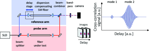
Figure 3$\cdot$1: Schematic of the experimental setup (SLD: superluminescent diode), and illustration of the cross-correlation trace expected at one pixel of the stack of images.

In the first set of experiments we employed free-space path for the reference beam (the dispersion of optical elements positioned in this path was negligible). A schematic of the setup is shown in Fig. 3$\cdot$1. The few-mode fiber under test is the final element of a module (L=0.6 m) consisting of a single-mode fiber, a TAP-LPG, and the higher-order mode fiber (L=0.4 m) [Ramachandran, 2005, Jespersen et al., 2010]. In this fiber, the LPG spectrum characterizes the mode conversion efficiency from the LP₀₁ core-mode to the LP₀₂ core-mode, which is used as an independent reference for comparison against the ratio of modal weights obtained by C²-imaging method.

The source spectrum, provided by an LED, was filtered by a bandpass with the central wavelength of about 780 nm and bandwidth of about 4 nm. Since the LPG mode-conversion bandwidth exceeds 20 nm, the wavelength-dependent LPG spectrum has a negligible impact on the spectra of HOM’s.

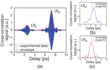
Figure 3$\cdot$2: (a): Cross-correlation trace for the entire image (data is offset corrected) for the bandpass centered at $\lambda_{center}$=780 nm. (b) and (c): fit of the model to the envelope of the experimental data, for the first and second peak, corresponding to LP₀₁ and LP₀₂, respectively.

Figure 3$\cdot$2(a) shows an example of cross-correlation trace between the reference field and the output of the fiber, integrated over all pixels of the camera. The peaks in the trace correspond to the two different modes in the HOM fiber. We analyze the data using elements of the theoretical analysis discussed in Chapter 2.

The envelope of the cross-correlation trace is obtained from the stack of images recorded by the camera, as shown in red color in Fig. 3$\cdot$2 (a). Then, the amplitude of the coherence function ${\cal G}_{rm}(\tau)$ is fitted to the extracted envelope, separately for the two peaks, as Figs. 3$\cdot$2(b) and (c) demonstrate.

The difference in shape of the two interference peaks reflects distinct modal dispersion of the corresponding modes. The side-lobes around the dominant peaks (clearly visible for the $LP_{02}$ mode) are due to the steep spectral edges of the filtered spectrum. By fitting ${\cal G}_{rm}(\tau)$ to these data, we obtain the relative group-delays and the dispersion of the two modes.

The dependence of the group-delay and dispersion on the wavelength is measured by shifting the central wavelength of the filtered spectrum (achieved by changing the incidence angle of light on the bandpass). The results are shown in Figs. 3$\cdot$3(a) and (b). For comparison, we have also simulated the modal properties of the tested fiber using a scalar mode-solver.

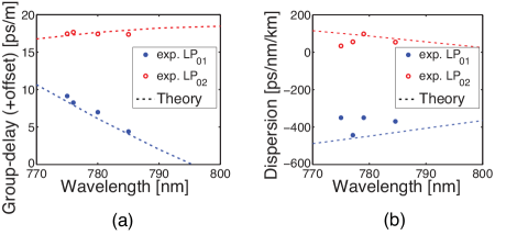
Figure 3$\cdot$3: (a) Group-delays, and (b) Dispersion values of the two modes as a function of center wavelength of the bandpass.

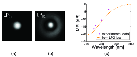
Figure 3$\cdot$4: (a) and (b), reconstructed $LP_{01}$ and $LP_{02}$-mode (gamma-adjusted) at a center wavelength of 780 nm, (c) multi-path interference (MPI) values as a function of center wavelength of the bandpass.

Figures 3$\cdot$4(a) and (b) show the reconstructed intensity distributions of $LP_{01}$ and $LP_{02}$ modes that match the expected pattern of the modes.

The relative (dispersion-corrected) weights of the normalized modes are characterized using the multi-path interference (MPI) value

$$MPI=10\log_{10}\left(p_{m}/p_{{}_{LP_{01}}}\right),$$ (3.1)

a useful measure of the relative power of a higher-order mode, $p_{m}$ to that of the fundamental mode $p_{{}_{LP_{01}}}$.

We demonstrate the accuracy of the C² imaging in Fig. 3$\cdot$4(c), where the multi-path interference (MPI) value is plotted as a function of the wavelength. The obtained MPI values match very well with the mode conversion efficiencies independently measured by recording the LPG spectrum.

3.2 Dispersion compensation for imaging of large-mode area fibers

The advantages of dispersion compensation are illustrated in characterization of large-mode-area (LMA) fibers supporting modes with similar dispersive characteristics. As I argued in Chapter 2, in this case, it is possible to achieve high temporal resolution of small intermodal group delays, although, obviously, at the expense of spectral resolution.

The temporal resolution of C²-imaging is related to the width of the coherence function ${\cal G}_{mr}(\tau)$, which is determined by the spectral properties of the light source. For a given shape of the spectrum, the temporal resolution $\Delta\tau_{FWHM}$ (defined here as the FWHM of ${\cal G}_{mr}(\tau)$) can be calculated as a function of the bandwidth of the spectrum and the residual group-velocity dispersion (GVD) $\Delta\varphi^{(2)}$.

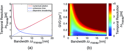
Figure 3$\cdot$5: (a) Temporal resolution as a function of the FWHM spectral bandwidth of a Gaussian spectrum (for GVD value of $\varphi^{(2)}=0.1ps^{2}$), (b) and as a function of both FWHM bandwidth and GVD.

We modeled the dependence of the temporal resolution for a Gaussian spectrum centered at 1060 nm and residual GVD of $\Delta\varphi^{(2)}=0.1ps^{2}$ (corresponding to about 4 m of LMA fiber and in the absence of the dispersion compensating fiber in the reference path). The results are shown in Fig. 3$\cdot$5(a).

For small bandwidths, dispersion plays a minor role, and the resolution is governed by the coherence time, which can be defined as $\Delta\tau_{FWHM}^{coh}=8\ln(2)/\Delta\omega_{FWHM}$, where $\Delta\omega_{FWHM}$ is the width of the spectrum at the angular frequency ($\Delta\omega_{FWHM}\approx 2\pi c_{0}\Delta\lambda_{FWHM}/\lambda_{0}^{2}$).

In the absence of dispersion, broad spectra may be used to achieve maximal temporal resolution. However, when the interferometer is not dispersion balanced, the broadening of cross-correlation signal is dominated by the dispersion, i.e. $\Delta\tau_{FWHM}^{disp}=\Delta\varphi^{(2)}\Delta\omega_{FWHM}$. Nonetheless, even in this case, it is possible to identify an optimal bandwidth of the spectrum (i.e. appropriate choice of the bandpass) corresponding to the optimal resolution, as Fig. 3$\cdot$5(b) clearly illustrates. The horizontal line in Fig. 3$\cdot$5(b) highlights the parameter configuration shown in Fig. 3$\cdot$5(a).

The temporal resolution may be noticeably improved in a dispersion-matched interferometer, a well-known result in optical coherence tomography (OCT) [Wojtkowski et al., 2004]. In our setup, we realize this idea by employing a single-mode fiber in the reference path, which balances the dispersion of the test fiber. Certainly, the dispersion can be exactly matched for a single mode or group of modes with similar dispersive characteristics. For the other modes, the residual dispersive phases cause broadening of the corresponding coherence peaks in the cross-correlation trace.

The shape and smoothness of the spectrum also have an impact on the cross-correlation trace, and thus, affect the temporal resolution. These effects have also been discussed in the context of OCT [de Boer et al., 2001].

For characterization of large-mode area (LMA) fibers, in which all the modes have similar magnitudes of chromatic dispersion and the relative delays are on a picosecond (or less) timescales, the results of dispersion-matching are particularly illuminating, as we demonstrate below.

We demonstrate dispersion compensation for characterization of the polarization-maintaining LMA fiber with a core diameter of approximately 27.5 $\mu m$ and a numerical aperture (NA) of 0.062, having the length of 5 m. We use a polarizer and a pair of half-wave plates to ensure launch of the beam into one of the dominant polarization states of the fiber. The dispersion is matched by using 4.08 meters of single-mode HI-1060 fiber in the reference path. This length has been determined by cutting the input of the reference fiber until the width of the dominant peak in the cross-correlation trace matched the coherence function calculated for the full spectrum of the source.

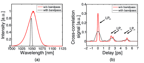
Figure 3$\cdot$6: (a): Full spectrum of the source and the 5-nm bandpass, (b): the envelopes of the cross-correlation traces.

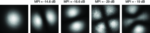
Figure 3$\cdot$7: Reconstructed mode profiles in the order of temporal delays shown in the cross-correlation trace of Fig. 3$\cdot$6 (b) for the case of the full spectrum of the source.

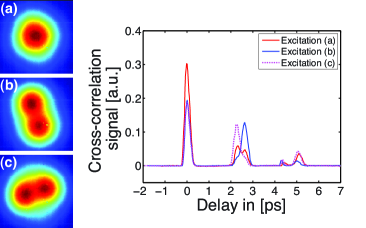
Figure 3$\cdot$8: (a-c) Output near-field images of the tested fiber, obtained for different in-coupling conditions, and corresponding changes in the cross-correlation trace.

The effect of dispersion-matching is clearly visible when comparing the cross-correlation traces, obtained using the full spectrum of the source in Fig. 3$\cdot$6(a), and those recorded using a spectrum filtered by a 5-nm bandpass filter in Fig. 3$\cdot$6(b). Most importantly, dispersion compensation combined with the use of full spectrum reveals the pairs of $LP_{11}$ and $LP_{21}$ modes, which overlap in the traces obtained using the filtered spectrum. The corresponding temporal resolution approaches values smaller than 300 fs. The impact of the shape of the spectrum on the cross-correlation trace is also noticeable: since the filtered spectrum has steep edges, the corresponding cross-correlation trace shows characteristic ringing (especially around the peak of the $LP_{01}$-mode). In contrast, the smooth full spectrum results in a cross-correlation trace without spectral artifacts.

Fig. 3$\cdot$7 demonstrates intensity distributions of all modes, arranged in the order of their time delay in Fig. 3$\cdot$6(b). The dispersion-corrected MPI values of the modes shown in Fig. 3$\cdot$6(b) (full spectrum) are estimated as -14.6 dB and -16.6 dB for the two $LP_{11}$ modes, and -29 dB and -19 dB for the two $LP_{21}$ modes. Interestingly, the dimensionless V-parameter of the test fiber is about 5, so the next higher $LP_{02}$-mode should also be present in the trace, but it is not observed in our measurements. Coiling of the fiber to a diameter of around 30 cm may be responsible for stripping off of the mode.

It is instructive to study the change of the modal pattern for different in-coupling conditions. A qualitative observation based upon the image of the output of the fiber in Fig. 3$\cdot$8(a), obtained when the reference beam is blocked, suggests fundamental-mode operation. Conversely, C²-imaging reveals that in fact the beam contains a significant amount of power in the higher-order modes. The evolution of the modal content for other in-coupling conditions measured by C²-imaging is illustrated in Fig. 3$\cdot$8. Here, the near-field image of the fiber-output in Fig. 3$\cdot$8(b) indicates a stronger excitation of the “slow” $LP_{11}$-mode, while Fig. 3$\cdot$8(c) shows a stronger “fast” $LP_{11}$-mode. Interestingly, in these two situations, $LP_{01}$-mode still carries most of the modal power.

These measurements also reveal that temporal splitting between the $LP_{21}$ modes is more pronounced compared to the splitting between the $LP_{11}$ modes. It is an indication that modes with higher orbital angular momentum (i.e. $LP_{lm}$ modes with higher $l$) are more susceptible to the birefringence effects in this polarization maintaining fiber [Golowich and Ramachandran, 2005].

3.3 Polarization reconstruction of vector modes

One of the major advantages of C²-imaging method compared to other waveguide characterization techniques [Nicholson et al., 2009] is the flexibility in choosing the polarization states of reference and signal beams independently of one another, as described in Chapter 2.

In this section, I employ this advantage of the method to characterize polarization properties of vector modes $TM_{01}$, $HE_{21}$, and $TE_{01}$ [Barankov et al., 2012b] propagating in the specialty fiber, where the degeneracy between the modes is lifted by the ingenious design of the index profile. The analysis is based on the formalism developed in Chapter 2.

The four vector modes propagating in the fiber can be represented in the following way:

$${\bf e}_{TM_{01}} = f(r)\left(\hat{x}\cos\varphi+\hat{y}\sin\varphi\right),$$

$${\bf e}_{TE_{01}} = f(r)\left(\hat{x}\sin\varphi-\hat{y}\sin\varphi\right),$$

$${\bf e}_{+} = f(r)e^{i\varphi}\left(\hat{x}+i\hat{y}\right)/\sqrt{2},$$

$${\bf e}_{-} = f(r)e^{-i\varphi}\left(\hat{x}-i\hat{y}\right)/\sqrt{2},$$ (3.2)

where $f(r)$ is the radial distribution of the modes that has characteristic “donut” shape; $\hat{x}$ and $\hat{y}$ are the unit vectors in the image plane. It is convenient to employ the cylindrical coordinate system, $x=r\cos\varphi$, $y=r\sin\varphi$, where $r$ is measured from the axis of the fiber, and $\varphi$ is the azimuthal angle.

The last two modes ${\bf e}_{\pm}\sim e^{\pm\varphi}$ are the degenerate orbital-angular-momentum (OAM) states characterized by the spatial phase $\varphi$ that encodes the orbital momentum $L_{z}=\pm 1$. Due to the spectral degeneracy, an arbitrary linear superposition of the modes defines $HE_{21}$ mode:

$${\bf e}_{HE_{21}}=c_{+}{\bf e}_{+}+c_{-}{\bf e}_{-},$$ (3.3)

where $c_{+}$ and $c_{-}$ are the complex-valued amplitudes of the modes normalized to unity, $|c_{+}|^{2}+|c_{-}|^{2}=1$. The amplitudes depend on the in-coupling conditions to the fiber.

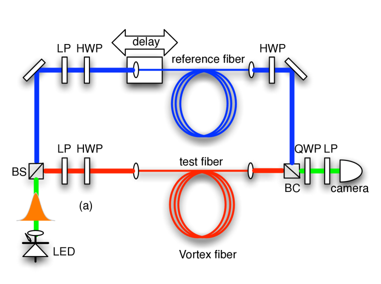
Figure 3$\cdot$9: C²-imaging setup: LED – light-emitting diode, LP-linear polarizer, HWP – half-wave plate, QWP – quarter-wave plate, BS – beam-splitter, BC – beam combiner.

The polarization-sensitive C²-imaging method is implemented using the experimental setup shown in Fig. 3$\cdot$9. I employ a pair of linear polarizers and half-wave plates to control the polarization state of the reference beam. The in-coupling conditions to the test fiber is also determined by a similar set of polarizing elements. Polarization selection at the output of the system is provided by a combination of a quarter-wave plate and a linear polarizer.

I used an LED source centered at about $\lambda=1524\,nm$ with spectral width of $\sim 30\,nm$. The output beam of the test fiber focused at the camera interferes with the collimated reference beam having well-defined linear polarization. The in-coupling conditions remain the same throughout our measurements. The length of the polarization-maintaining reference fiber is chosen to match the optical paths of the two beams and also to compensate for the modal dispersion of the test fiber. The effect of dispersion has been also minimized by using a spectral filter with a central wavelength of $\lambda\approx 1549\,nm$ and width $\lambda_{FWHM}\approx 6\,nm$. The camera detects a cross-correlation signal as a function of the group delay monitored by a computer-controlled delay stage. In the measurements, the cross-correlation trace has been recorded for three pairs of orthogonal polarization states of the reference beam: linear vertical, linear horizontal, linear at $+\pi/4$ radians, linear at $-\pi/4$ radians, left-circular and right-circular polarizations. The envelopes of the cross-correlation traces have been analyzed to study the polarization properties and the relative power of the modes.

Among the six polarization states used in the experiment, the left-circular and right-circular states are particularly important for identifying the topological charge of the OAM state. Specifically, as Fig. 3$\cdot$10 illustrates, $TE_{01}$ and $TM_{01}$ modes are insensitive to changes in orientation of the circular polarizer, as dictated by their spatial and polarization properties. In contrast, the two OAM states with the orbital angular momentum $L_{z}=\pm 1$, have the right and left circular polarizations, correspondingly. Therefore, one can detect each of these states using a circular polarizer, as shown in Fig. 3$\cdot$10. The peak values of the thus-recorded cross-correlation traces contain the relative weights of the two OAM’s, and also the weights of the other two modes.

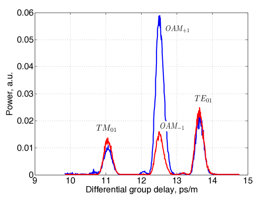
Figure 3$\cdot$10: Relative modal power as a function of group delay: blue line – right-circular polarization, red line – left- circular polarization

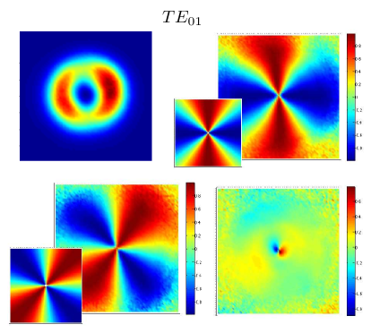
Figure 3$\cdot$11: Reconstruction of Stokes parameters of $TE_{01}$ mode: (a) component $S_{0}$, (b) component $S_{1}$, (c) component $S_{2}$, (d) component $S_{3}$. Inset: theoretical prediction.

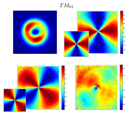
Figure 3$\cdot$12: Reconstruction of Stokes parameters of $TM_{01}$ mode: (a) component $S_{0}$, (b) component $S_{1}$, (c) component $S_{2}$, (d) component $S_{3}$. Inset: theoretical prediction.

Polarization-sensitive imaging method described in Chapter 2 allows complete reconstruction of the Stokes parameters of $TM_{01}$, $TE_{01}$, and $HE_{21}$ modes and direct comparison to the theoretical predictions based upon polarization patterns shown in Eqs. (3.3) and (3.3).

Specifically, for $TM_{01}$ the Stokes vector components are

$$S_{0}({\bf r})=f(r),\,S_{1}({\bf r})=-f(r)\cos(2\varphi),\,S_{2}({\bf r})=f(r)\sin(2\varphi),\,S_{3}({\bf r})=0.$$ (3.4)

Similarly, for $TE_{01}$, one obtains

$$S_{0}({\bf r})=f(r),\,S_{1}({\bf r})=f(r)\cos(2\varphi),\,S_{2}({\bf r})=-f(r)\sin(2\varphi),\,S_{3}({\bf r})=0.$$ (3.5)

In the most interesting case of $HE_{21}$ mode, the Stokes parameters $S_{1}$ and $S_{2}$ encode the interference term $c_{+}c^{*}_{-}=|c_{+}c_{-}|e^{i\alpha}$ of the two degenerate OAM states

$$S_{0}({\bf r}) = f(r),\,S_{1}({\bf r})=2|c_{+}c_{-}|f(r)\cos(2\varphi+\alpha),$$

$$S_{2}({\bf r}) = -2|c_{+}c_{-}|f(r)\sin(2\varphi+\alpha),\,S_{3}({\bf r})=|c_{+}|^{2}-|c_{-}|^{2}$$ (3.6)

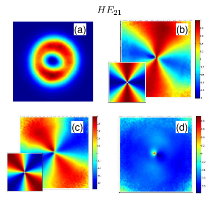
Figure 3$\cdot$13: Reconstruction of Stokes parameters of $HE_{21}$ mode: (a) component $S_{0}$, (b) component $S_{1}$, (c) component $S_{2}$, (d) component $S_{3}$. Inset: theoretical prediction

The intensity distribution of each mode, given by the component $S_{0}$ of the spatially dependent Stokes vector, as expected, demonstrates characteristic donut shape, as illustrated in Figs. 3$\cdot$11, 3$\cdot$12, and 3$\cdot$13.

In summary, the reconstructed Stokes parameters for all vector modes compare very well with the theoretical predictions. In addition, phase patterns $S_{1}$ and $S_{2}$ in Fig. 3$\cdot$13 reveal the relative phase of the degenerate OAM states ${\bf e}_{\pm}$.

3.4 Spatial phase reconstruction of vortex modes

Polarization properties of OAM states shown in Eqs.(3.3) suggest a simple method to measure their modal power. Indeed, by projecting the output beam to the left and right circular polarized states, one obtains the cross-correlation traces of the states independently of one another. Moreover, since the other two vector states, $TM_{01}$ and $TE_{01}$, are insensitive to the change of the circular polarization, these states can be easily identified and separated in the cross-correlation traces, as shown in Fig. 3$\cdot$10.

One of the key characteristics of OAM states

$${\bf e}_{+} = f(r)e^{i\varphi}\left(\hat{x}+i\hat{y}\right)/\sqrt{2},$$

$${\bf e}_{-} = f(r)e^{-i\varphi}\left(\hat{x}-i\hat{y}\right)/\sqrt{2},$$ (3.7)

is the phase factor $e^{\pm i\varphi}$ corresponding to the two eigen-values of orbital momentum $L_{z}=\pm 1$ along the direction of propagation.

In this section, I apply the phase-sensitive C²-imaging to measure the phase distribution of the vortex states [Barankov et al., 2012a]. First, I project the interferometric signal onto the right- and left- circular polarization states to select the two vortex states independent of one another. The resulting interferometric trace contains the information about the spatial phase that can be retrieved using simple phase-stepping algorithm developed in Chapter 2.

The cross-correlation signal is measured with high temporal resolution corresponding to a fraction of the wavelength in spatial translation of the delay stage. The phase-stepping algorithm is capable of retrieving the phase information even for relatively noisy conditions.

The results of phase reconstruction of the OAM states are shown in Figs. 3$\cdot$14 and 3$\cdot$15 for $L_{z}=+1$ and $L_{z}=-1$ states, correspondingly. The spatial pattern reveals clockwise and counterclockwise phase wrapping, which uniquely identifies the two states. The position of the phase discontinuity in Figs. 3$\cdot$14 and 3$\cdot$15 allows direct measurement of the relative phase of the states.

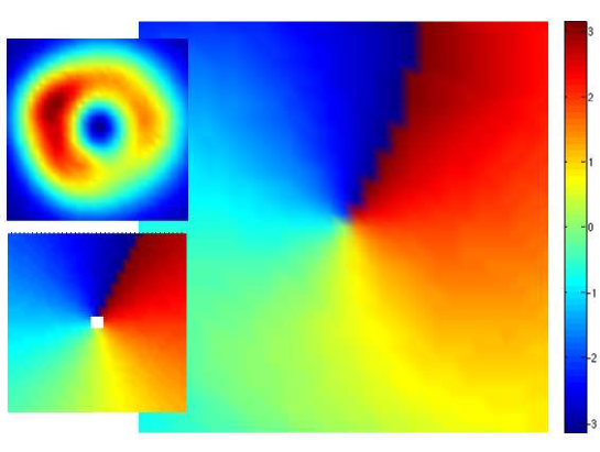
Figure 3$\cdot$14: Spatial phase of OAM state with $L_{z}=+1$ that shows characteristic phase wrapping in the counter-clockwise direction. Insets: (a) Intensity distribution of the mode, (b) theoretical distribution of spatial phase

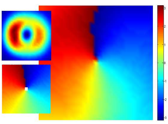
Figure 3$\cdot$15: Spatial phase of OAM state with $L_{z}=-1$ that shows characteristic phase wrapping in the clockwise direction. Insets: (a) Intensity distribution of the mode, (b) theoretical distribution of spatial phase

In summary, OAM states propagating in optical waveguides demonstrate distinct polarization and spatial patterns. Using polarization and phase-sensitive C²-imaging methods, I have completely characterized these modes, revealing their unique polarization and phase singularities, the modal power and also the relative phase of the states.

3.5 Resonant mode coupling in leakage channel fibers

For an updated description of this experiment, I refer the reader to a recent preprint “Resonant Bend Loss in Leakage Channel Fibers” by R. A. Barankov, K. Wei, B. Samson, and S. Ramachandran posted at arXiv:1205.5584v1 [physics.optics]. Below is the original write-up as submitted to the library of Boston University.

In this section, I describe modal characterization of large-mode-area leakage channel fibers, which demonstrate dramatic power loss at certain coiling radius. Using C²-imaging, I experimentally attribute this anomaly to a new physical mechanism of resonant mode-coupling [Barankov et al., 2012c].

Resonantly enhanced leakage-channel fibers (LCFs) with large mode areas are designed to provide high-power propagation of diffraction-limited beams in high-power fiber lasers [Dong et al., 2009]. The microstructure of these fibers is tailored to enhance the loss of higher-order modes (HOMs) while maintaining tolerable loss of the fundamental mode, resulting in single-mode operation with large field diameters. In the existing designs [Dong et al., 2009], the boundary between the light-guiding core and the cladding consists of low-index circular rods, so that index-continuity of the boundary in the azimuthal direction is broken. As a result, all modes propagating in the fiber are coupled to the radiative modes of the cladding. However, the presence of gaps at the interface naturally promotes significant differential power-loss dominated by HOMs. A careful study of the mechanism and different possible fiber-designs indicates that high confinement loss for HOMs and low confinement loss for the fundamental mode can be achieved, leading to effectively single-mode operation of the structures [Dong et al., 2009].

The physical mechanism underlying the LCF design suggests sensitivity of light propagation to the coiling conditions of the fibers. Indeed, it is well-known that coiled fibers experience power loss resulting from bend-induced coupling of the guided modes to the radiative modes of the cladding [Marcuse, 1976, Wong et al., 2005, Dong et al., 2006, Saitoh et al., 2011]. In this case, the loss is significantly higher for HOMs than for the fundamental mode, as dictated by larger modal overlap of HOMs and the cladding modes. Moreover, when the cladding modes become quasi-guided in coated fibers [Renner, 1992], a resonant behavior is observed [Murakami and Tsuchiya, 1978].

The bend-loss becomes significant for small enough coiling radii [Love, 1989]. The critical radius has been estimated in the case of photonic-crystal fibers [Birks et al., 1997] as $R_{c}\sim\Lambda^{3}/\lambda^{2}$ in the short-wavelength limit, where $\lambda$ is the wavelength of light, and $\Lambda$ is the characteristic core size [Birks et al., 1997, Nielsen et al., 2004]. This estimate should also hold for leakage-channel fibers characterized by similar geometry. For example, for the LCFs with core size $\Lambda\sim 50\,{\rm\mu m}$, significant bend loss is expected at $R_{c}\sim 10\,{\rm cm}$ in the $1\,{\rm\mu m}$ spectral range.

In addition to the power-loss resulting from direct radiative coupling of the core modes, bending of fibers induces inter-modal coupling in the core [Russell, 2006, Love and Durniak, 2007]. The coupling increases dramatically when the effective indices of the two modes approach one another as a function of the fiber curvature. The crossing occurs at some critical radius, which, in general, depends on the properties of the coupled modes. Interestingly, the crossing between the fundamental and the lowest HOM is also expected at the critical radius $R_{c}$ corresponding to onset of significant bend-loss [Russell, 2006].

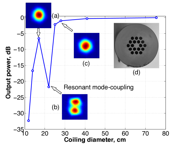
Figure 3$\cdot$16: Output power as a function of coiling diameter. Insets (a-c): Output mode profiles at different coiling diameters; (d) Cross-section of the LCF

In this work, we explore the effect of resonant mode-coupling on the bend-loss in a large-mode area LCF and observe an enhanced power loss at a certain coiling diameter. The results of power measurements in the $1\,{\rm\mu m}$ spectral range are shown in Fig. 3$\cdot$16. We observe a dramatic decrease of the output light power at a specific coiling diameter, while the power recovers to the levels offset by the usual mechanism of power loss outside the resonance. At small coiling radii, as expected, one obtains significant loss of power in accord with the usual bend-loss mechanism [Marcuse, 1976, Birks et al., 1997]. We characterize the observed anomaly by C²-imaging method [Schimpf et al., 2011]. Specifically, we find that for non-critical coiling radii, light propagation in the tested LCF is dominated by the fundamental mode with HOM extinction below $-25\,{\rm dB}$. Thus, at non-critical radii the power-loss can be explained by the usual bend-loss mechanisms [Birks et al., 1997, Russell, 2006]. In contrast, at the critical coiling radius, a higher-order mode dominates propagation, indicating resonant coupling of the fundamental mode to HOMs, which, by the design of LCFs, immediately radiate out of the core. Interestingly, this mechanism is reminiscent of resonant mode coupling observed in coated single-mode fibers [Renner, 1992]. While simple bend-loss measurements shown in Fig. 3$\cdot$16 reveal this anomalous behavior, C²-imaging method allows us to quantify this effect. As a result, this precise characterization method provides critical feedback for future fiber-designs, in which the critical radius $R_{c}$ should be defined for specific amplifier packaging constraints.

The tested LCF of $285\,{\rm cm}$-length has a core diameter of $50\,{\rm\mu m}$ and cladding diameter of $400\,{\rm\mu m}$. The two rings of low-index (fluorine-doped) silica regions shown in Fig. 3$\cdot$17(a) provide the leakage channel. The core, made of silica, is index matched to the outer silica glass. A high-index regular acrylate coating applied to the cladding ensures stripping out of the cladding modes. The LCF has been designed to have negligible HOM content at lengths greater than $3\,{\rm m}$. The input end of the fiber was spliced to a single-mode fiber to provide same in-coupling conditions throughout the experiments.

The modal content of the LCF was analyzed using C²-imaging method developed in Chapter 2. The basic idea of the method is to study the interference of the beam radiated from an optical waveguide with an external reference beam, and detect different waveguide modes in the time-domain by changing the relative optical paths of the two beams.

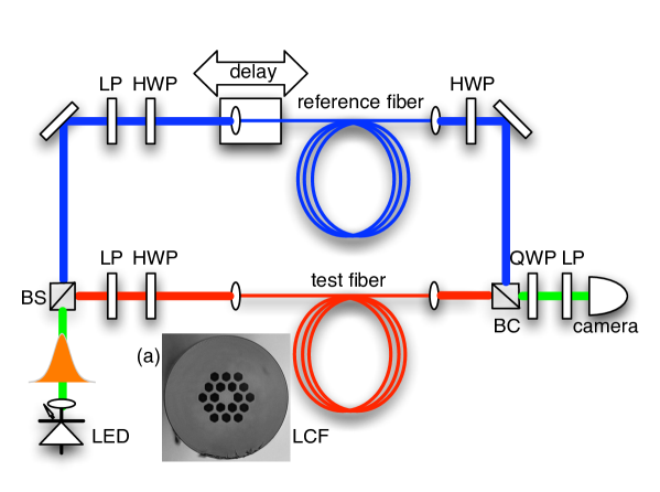
Figure 3$\cdot$17: C²-imaging setup: LED – light-emitting diode, LP-linear polarizer, HWP – half-wave plate, QWP – quarter-wave plate, BS – beam-splitter, BC – beam combiner. Inset (a): Cross-section of the LCF

Figure 3$\cdot$17 shows a schematic diagram of the experimental setup based on a Mach-Zehnder interferometer. We used a superluminescent diode (SLD) source centered at $\lambda\sim 1050\,{\rm nm}$ with a spectral width of $\sim 30\,{\rm nm}$. The output beam of the LCF (focused at the imaging plane) interferes with the collimated reference beam radiated from the reference fiber. The length of polarization-maintaining reference fiber is chosen to compensate for the optical path difference between the two paths and also to reduce the effects of group-velocity dispersion of the LCF. The latter is important since we employ a light source with a relatively broad spectrum, which, in the absence of dispersion compensation, leads to significant dispersion broadening of the cross-correlation signal. In particular, the mode-specific resolution of C²-imaging method is defined by the spectral width of the source and also by the dispersion mismatch of the reference and the test modes. In large-mode-area LCFs, the material dispersion dominates the spectral broadening, which results in similar dispersion properties of HOMs. We chose the length of the reference fiber to match the material dispersion of LCF and, thus, reduced the dispersive broadening of all the modes simultaneously.

The cross-correlation signal ${\cal P}({\bf r},\tau)$ as a function of the group delay $\tau$ and the coordinate ${\bf r}$ in the imaging plane is detected by the camera for different positions $d=c\tau$ ($c$ is the speed of light in vacuum) of the delay stage:

$${\cal P}({\bf r},\tau)=\sum_{m}p_{m}{\cal G}_{mr}^{2}(\tau-\tau_{mr})I_{m}({\bf r}).$$ (3.8)

Here, the summation extends over the modes propagating in LCF, $p_{m}$ is the relative modal power of $m$-th mode ($\sum_{m}p_{m}=1$), ${\cal G}_{mr}(\tau)$ is the mutual coherence function of the reference and test beams, $I_{m}({\bf r})$ is the modal intensity, and $\tau_{mr}$ is the relative group delay of the $m$-th mode with respect to the reference mode.

Coiling of the fiber affects polarization properties of the test beam. To extract the power of every elliptically-polarized mode, we have recorded the cross-correlation trace for two orthogonal polarization states of the reference beam. The resulting trace, combining the two measurements, is represented in Eq. (3.8). The modal intensity distribution $I_{m}({\bf r})$ of every mode was obtained by integrating this expression over the time extent of the mode. The relative power of the modes is encoded in the net cross-correlation trace obtained by integration of the spatially-dependent trace in Eq. (3.8) over the imaging plane position.

The result of this procedure, applied to the cross-correlation traces recorded at the critical coiling radius, is shown in Fig. 3$\cdot$18. In this figure, the cross-correlation peaks identify the modes propagating in the fiber at the corresponding relative group delays. The shape of the peaks reflects the corresponding mutual coherence functions, while the peak values encode the relative power of the modes. The insets demonstrate the intensities of the reconstructed modes.

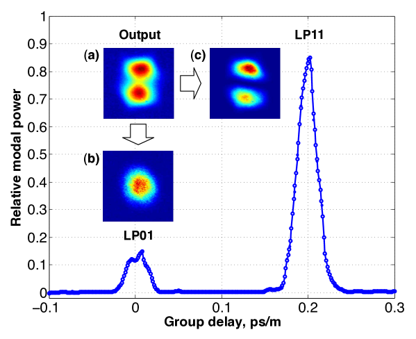
Figure 3$\cdot$18: Relative modal power as a function of group delay at the resonance (D=22cm). Insets: output image and the images of reconstructed modes

The dependence of the output power on the coiling diameter was measured using a power meter. The results are shown in Fig. 3$\cdot$16. We observe a dramatic decrease of the output light power at a specific coiling diameter. The observed critical radius $R_{exp}\approx 11\,{\rm cm}$ is close to the estimate $R_{c}\sim 10\,{\rm cm}$, suggesting resonant mode-coupling as the mechanism responsible for the anomalous power loss. Indeed, at the resonance, the output image demonstrates domination of HOM’s as shown in Fig. 3$\cdot$16(b), while the output images in Fig. 3$\cdot$16(a) and 3$\cdot$16(c), recorded at coiling diameters outside the resonance, indicate single-mode operation.

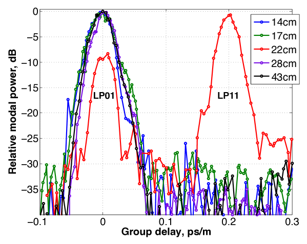
Figure 3$\cdot$19: Relative modal power of $LP_{01}$ and $LP_{11}$ (peak values) as a function of the relative group delay, for different coiling diameters

C²-imaging [Schimpf et al., 2011] provides insight into the resonant behavior. The envelope of the integrated correlation trace shown in Fig. 3$\cdot$18 at the critical coiling diameter demonstrates two modes ($LP_{01}$ and $LP_{11}$) propagating with a relative group delay of about $0.2\,{\rm ps/m}$, with the fundamental mode contributing only about 15% of the total power. In contrast, at other coiling diameters, HOM’s are suppressed at the power level below $-25\,{\rm dB}$, as shown in Fig. 3$\cdot$19. The strength of the resonance depends on the length of the coiled fiber. In a set of similar measurements conducted on the LCF of smaller length of about $180\,{\rm cm}$, a relatively shallow resonance was found at the same coiling diameter. We expect a significantly deeper resonance for longer fiber lengths.

In summary, coiled few-mode fibers experience bend-induced coupling between the core modes and power-loss via direct coupling of core modes to the radiative modes of the cladding. Using C²-imaging, we explore the interplay of these phenomena in LCFs. We identify a new resonant power-loss mechanism in these fibers, in which higher-order core modes mediate coupling of the fundamental mode to the radiative modes. The effect becomes evident at a specific coiling diameter, where we observe a dramatic decrease of the output power. Outside the resonance, the power recovers to the levels determined by the usual bend-loss mechanism. In this work, we quantify this anomaly by C²-imaging, thus providing critical feedback for the fiber-based amplifier designs with certain coiling constraints.

Chapter 4 Conclusions

In this work, I have developed a novel interferometric method, called C²-imaging, suitable for complete characterization of waveguide modes. In particular, using this method one obtains the modal weights, relative group delays and dispersion properties of the modes. Modifications of the method, involving polarization post-selection and the analysis of high-frequency oscillations of interferometric signal, reveal polarization and phase distributions of all the modes.

The developed method has been successfully applied to modal characterization of waveguides with distinct modal properties. In particular, in a specialty higher-order mode fiber, the method allowed accurate reconstruction of the modes having small relative group delays and distinct dispersive behavior. The reconstructed modal weights agree well with the mode-conversion of the long-period grating spectrum. The multi-path interference values down to $-30\,{\rm dB}$ can be accurately retrieved. The concept of dispersion-compensation was demonstrated in the case of large-mode-area fibers, where sufficient temporal resolution was achieved to observe temporal birefringent splitting between odd and even higher order modes propagating in the polarization maintaining fiber.

Polarization-sensitive modification of C²-imaging method was successfully tested for modal characterization of a specialty fiber supporting several vector modes. The reconstructed polarization patterns, demonstrating non-trivial space dependence, compare very well with the theoretical predictions. In addition, I have directly observed optical orbital angular momentum states propagating in the fiber, by employing circular polarization selectivity of the modes. The observed phase patterns of the modes are consistent with the theoretical expectations for the corresponding spatially dependent Stokes parameters.

Phase-sensitivity of C²-imaging was also demonstrated in the experiments with the same specialty fiber. I have directly measured, for the first time to the best of my knowledge, the phase distribution of the orbital momentum states, using a phase-retrieval algorithm based upon analysis of high-frequency oscillations of the interferometric cross-correlation signal. As a result, I have completely characterized the vortex modes and identified their relative power and the complex relative phase.

I have also used C²-imaging to explore the resonant behavior of power output in large-mode-area leakage-channel fibers. In particular, I have identified the resonant mode-coupling as the mechanism responsible for the observed dramatic power loss at a specific coiling radius.

The versatility of C² imaging, demonstrated in this work, identifies this method as a powerful new tool, suitable for waveguide characterization in optical applications.

I kindly acknowledge support of this project by ARL Grant No. W911NF-06-2-0040, ONR Grant Nos. N00014-11-1-0133 and N00014-11-1-0098.

Education

2012	Boston University, Boston, Massachusetts
	– M.S. in Electrical Engineering (May 2012),
	Research advisor – Prof. Siddharth Ramachandran
2006	Massachusetts Institute of Technology, Cambridge, Massachusetts
	– Ph.D. in Physics
	Research advisor – Prof. Leonid Levitov
1998	Moscow Engineering Physics Institute, Moscow, Russia
	– Diploma with honors in Physics

Employment

2007-2012	Boston University, Boston, Massachusetts
	– Research Assistant at the Department of Electrical and Computer Engineering
	– Research Scientist at the Physics Department
2010-2012	Simmons College, Boston, Massachusetts
	– Lecturer at the Department of Chemistry and Physics
2005-2007	University of Illinois at Urbana-Champaign, Urbana, Illinois
	– Postdoctoral Research Associate at the Physics Department
2002-2005	Massachusetts Institute of Technology, Cambridge, Massachusetts
	– Research Assistant at the Department of Physics

Research Area

Applied Optics: interferometric methods for waveguide characterization
Theoretical condensed matter and atomic physics:
many-body dynamics of cold atoms and quantum fluids

Related Professional Experience

Member of the American Physical Society (since 2003)
Referee for Physical Review Letters and Physical Review A

Journal Publications

• “Cross-correlated ($C^{2}$) imaging of fiber and waveguide modes”, D. N. Schimpf, R. A. Barankov, and S. Ramachandran, Optics Express 19, Issue 14, pp. 13008-13019 (2011).

• “Adiabatic nonlinear probes of one-dimensional Bose gases”, C. De Grandi, R. A. Barankov, and A. Polkovnikov, Phys. Rev. Lett. 101, 230402 (2008).

• “Optimal non-linear passage through a quantum critical point”, Roman Barankov and Anatoli Polkovnikov, Phys. Rev. Lett. 101, 076801 (2008).

• “Phase-Slip Avalanches in the Superflow of ⁴He through Arrays of Nanosize Apertures”, David Pekker, Roman Barankov, and Paul M. Goldbart, Phys. Rev. Lett. 98, 175301 (2007).

• “Coexistence of Superfluid and Mott Phases of Lattice Bosons”, R. A. Barankov, C. Lannert, and S. Vishveshwara, Phys. Rev. A 75, 063622 (2007).

• “Synchronization in the BCS Pairing Dynamics as a Critical Phenomenon”, R. A. Barankov and L. S. Levitov, Phys. Rev. Lett. 96, 230403 (2006).

• “Dynamical Selection in Emergent Fermionic Pairing”, R. A. Barankov and L. S. Levitov, Phys. Rev. A 73, 033614 (2006).

• “Atom-molecule Coexistence and Collective Dynamics near a Feshbach Resonance of Cold Fermions”, R. A. Barankov and L. S. Levitov, Phys. Rev. Lett. 93, 130403 (2004).

• “Solitons and Rabi Oscillations in a Time-Dependent BCS Pairing Problem”, R. A. Barankov, L. S. Levitov and B. Z. Spivak, Phys. Rev. Lett. 93, 160401 (2004).

• “Dissipative Dynamics of a Josephson Junction in the Bose-Gases”,
  R. A. Barankov and S. N. Burmistrov, Phys. Rev. A 67, 013611 (2003).

• “Boundary of Two Mixed Bose-Einstein Condensates”, R. A. Barankov, Phys. Rev. A 66, 013612 (2002).

Bibliography

- Barankov et al., 2012a Barankov, R. A., Kristensen, P., and Ramachandran, S. (2012a). Direct observation of orbital angular momentum states in fibers. in preparation.
- Barankov et al., 2012b Barankov, R. A., Kristensen, P., and Ramachandran, S. (2012b). Polarization reconstruction of vector modes using cross-correlation-imaging. in preparation.
- Barankov and Ramachandran, 2012 Barankov, R. A. and Ramachandran, S. (2012). Cross-correlation imaging for waveguide characterization. in preparation.
- Barankov et al., 2012c Barankov, R. A., Wei, K., Samson, B., and Ramachandran, S. (2012c). Anomalous bend loss in large-mode area leakage channel fibers. in preparation.
- Berdagué and Facq, 1982 Berdagué, S. and Facq, P. (1982). Mode division multiplexing in optical fibers. Applied Optics, 21(11):1950–1955.
- Birks et al., 1997 Birks, T. A., Knight, J. C., and Russell, P. S. (1997). Endlessly single-mode photonic crystal fiber. Optics Letters, 22(13):961–963.
- de Boer et al., 2001 de Boer, J. F., Saxer, C. E., and Nelson, J. S. (2001). Stable carrier generation and phase-resolved digital data processing in optical coherence tomography. Applied Optics, 40(31):5787–5790.
- Dong et al., 2006 Dong, L., Li, J., and Peng, X. (2006). Bend-resistant fundamental mode operation in ytterbium-doped leakage channel fibers with effective areas up to 3160. Optics Express, 14(24):11512–11519.
- Dong et al., 2009 Dong, L., Mckay, H. A., Marcinkevicius, A., Fu, L., Li, J., Thomas, B. K., and Fermann, M. E. (2009). Extending effective area of fundamental mode in optical fibers. Journal of Lightwave Technology, 27(11):1565–1570.
- Feder et al., 2003 Feder, K., Westbrook, P., Ging, J., Reyes, P., and Carver, G. (2003). In-fiber spectrometer using tilted fiber gratings. IEEE Photonics Technology Letters, 15(7):933 –935.
- Galvanauskas et al., 2008 Galvanauskas, A., Swan, M. C., and Liu, C.-H. (2008). Effectively single-mode large core passive and active fibers with chirally coupled-core structures. In CLEO/QELS 08: Conference on Lasers and Electro-Optics, 2008 and 2008 Conference on Quantum Electronics and Laser Science/San Jose. Piscataway, NJ: IEEE, page CMB1.
- Golowich and Ramachandran, 2005 Golowich, S. and Ramachandran, S. (2005). Impact of fiber design on polarization dependence in microbend gratings. Optics Express, 13(18):6870–6877.
- Golowich et al., 2004 Golowich, S. E., Reed, W. A., and Ritger, A. J. (2004). A new modal power distribution measurement for high-speed short-reach optical systems. Journal of Lightwave Technology, 22(2):457.
- Hanzawa et al., 2011 Hanzawa, N., Saitoh, K., Sakamoto, T., Matsui, T., Tomita, S., and Koshiba, M. (2011). Demonstration of mode-division multiplexing transmission over 10 km two-mode fiber with mode coupler. In Optical Fiber Communication Conference, page OWA4. Optical Society of America.
- Jespersen et al., 2010 Jespersen, K. G., Le, T., Grüner-Nielsen, L., Jakobsen, D., Pederesen, M. E. V., Smedemand, M. B., Keiding, S. R., and Palsdottir, B. (2010). A higher-order-mode fiber delivery for ti:sapphire femtosecond lasers. Optics Express, 18(8):7798–7806.
- Koplow et al., 2000 Koplow, J. P., Kliner, D. A. V., and Goldberg, L. (2000). Single-mode operation of a coiled multimode fiber amplifier. Optics Letters, 25(7):442–444.
- Love, 1989 Love, J. (1989). Application of a low-loss criterion to optical waveguides and devices. IEE Proceedings Optoelectronics, 136(4):225 –228.
- Love and Durniak, 2007 Love, J. and Durniak, C. (2007). Bend loss, tapering, and cladding-mode coupling in single-mode fibers. IEEE Photonics Technology Letters, 19(16):1257 –1259.
- Ma et al., 2009 Ma, Y., Sych, Y., Onishchukov, G., Ramachandran, S., Peschel, U., Schmauss, B., and Leuchs, G. (2009). Fiber-modes and fiber-anisotropy characterization using low-coherence interferometry. Applied Physics B: Lasers and Optics, 96:345–353. 10.1007/s00340-009-3517-9.
- Marcuse, 1976 Marcuse, D. (1976). Curvature loss formula for optical fibers. Journal of the Optical Society of America, 66(3):216–220.
- Menashe et al., 2001 Menashe, D., Tur, M., and Danziger, Y. (2001). Interferometric technique for measuring dispersion of high order modes in optical fibres. Electronics Letters, 37(24):1439 –1440.
- Murakami and Tsuchiya, 1978 Murakami, Y. and Tsuchiya, H. (1978). Bending losses of coated single-mode optical fibers. IEEE Journal of Quantum Electronics, 14(7):495 – 501.
- Nandi et al., 2009 Nandi, P., Chen, Z., Witkowska, A., Wadsworth, W. J., Birks, T. A., and Knight, J. C. (2009). Characterization of a photonic crystal fiber mode converter using low coherence interferometry. Optics Letters, 34(7):1123–1125.
- Nicholson et al., 2009 Nicholson, J., Yablon, A., Fini, J., and Mermelstein, M. (2009). Measuring the modal content of large-mode-area fibers. IEEE Journal of Selected Topics in Quantum Electronics, 15(1):61 –70.
- Nicholson et al., 2008 Nicholson, J. W., Yablon, A. D., Ramachandran, S., and Ghalmi, S. (2008). Spatially and spectrally resolved imaging of modal content in large-mode-area fibers. Optics Express, 16(10):7233–7243.
- Nielsen et al., 2004 Nielsen, M., Mortensen, N., Albertsen, M., Folkenberg, J., Bjarklev, A., and Bonacinni, D. (2004). Predicting macrobending loss for large-mode area photonic crystal fibers. Optics Express, 12(8):1775–1779.
- Ramachandran, 2005 Ramachandran, S. (2005). Dispersion-tailored few-mode fibers: a versatile platform for in-fiber photonic devices. Journal of Lightwave Technology, 23(11):3426 – 3443.
- Ramachandran et al., 2005 Ramachandran, S., Ghalmi, S., Bromage, J., Chandrasekhar, S., and Buhl, L. (2005). Evolution and systems impact of coherent distributed multipath interference. IEEE Photonics Technology Letters, 17(1):238 –240.
- Ramachandran et al., 2003 Ramachandran, S., Nicholson, J., Ghalmi, S., and Yan, M. (2003). Measurement of multipath interference in the coherent crosstalk regime. IEEE Photonics Technology Letters, 15(8):1171 –1173.
- Ramachandran et al., 2006 Ramachandran, S., Nicholson, J. W., Ghalmi, S., Yan, M. F., Wisk, P., Monberg, E., and Dimarcello, F. V. (2006). Light propagation with ultralarge modal areas in optical fibers. Optics Letters, 31(12):1797–1799.
- Renner, 1992 Renner, H. (1992). Bending losses of coated single-mode fibers: a simple approach. Journal of Lightwave Technology, 10(5):544 –551.
- Richardson et al., 2010 Richardson, D. J., Nilsson, J., and Clarkson, W. A. (2010). High power fiber lasers: current status and future perspectives, invited. Journal of the Optical Society of America B, 27(11):B63–B92.
- Rittich, 1985 Rittich, D. (1985). Practicability of determining the modal power distribution by measured near and far fields. Journal of Lightwave Technology, 3(3):652 – 661.
- Russell, 2006 Russell, P. S. (2006). Photonic-crystal fibers. Journal of Lightwave Technology, 24(12):4729–4749.
- Ryf et al., 2011 Ryf, R., Randel, S., Gnauck, A. H., Bolle, C., Essiambre, R.-J., Winzer, P., Peckham, D. W., McCurdy, A., and Lingle, R. (2011). Space-division multiplexing over 10 km of three-mode fiber using coherent mimo processing. In Optical Fiber Communication Conference, page PDPB10. Optical Society of America.
- Saitoh et al., 2011 Saitoh, K., Varshney, S., Sasaki, K., Rosa, L., Pal, M., Paul, M. C., Ghosh, D., Bhadra, S. K., and Koshiba, M. (2011). Limitation on effective area of bent large-mode-area leakage channel fibers. Journal of Lightwave Technology, 29(17):2609–2615.
- Salsi et al., 2011 Salsi, M., Koebele, C., Sperti, D., Tran, P., Brindel, P., Mardoyan, H., Bigo, S., Boutin, A., Verluise, F., Sillard, P., Bigot-Astruc, M., Provost, L., Cerou, F., and Charlet, G. (2011). Transmission at 2x100gb/s, over two modes of 40km-long prototype few-mode fiber, using lcos based mode multiplexer and demultiplexer. In Optical Fiber Communication Conference, page PDPB9. Optical Society of America.
- Schimpf et al., 2011 Schimpf, D. N., Barankov, R. A., and Ramachandran, S. (2011). Cross-correlated (c2) imaging of fiber and waveguide modes. Optics Express, 19(14):13008–13019.
- Siegman, 1990a Siegman, A. E. (1990a). Defining, measuring, and optimizing laser beam quality. Proceedings of SPIE, 1868:2.
- Siegman, 1990b Siegman, A. E. (1990b). New developments in laser resonators. Proceedings of SPIE, 1224:2.
- Stutzki et al., 2011 Stutzki, F., Jansen, F., Eidam, T., Steinmetz, A., Jauregui, C., Limpert, J., and Tünnermann, A. (2011). High average power large-pitch fiber amplifier with robust single-mode operation. Optics Letters, 36(5):689–691.
- Wagener et al., 1997 Wagener, J. L., Strasser, T. A., Pedrazzani, J. R., DeMarco, J., and DiGiovanni, D. J. (1997). Fiber grating optical spectrum analyser tap. IOOC-ECOC97: 11th International Conference on Integrated Optics and Optical Fibre Communications. 23rd European Conference on Optical Communications, 22-25 September 1997. IEE Conference Publication 448. London: Institution of Electrical Engineers., pages 65–68.
- Westbrook et al., 2000 Westbrook, P., Strasser, T., and Erdogan, T. (2000). In-line polarimeter using blazed fiber gratings. IEEE Photonics Technology Letters, 12(10):1352 –1354.
- Wielandy, 2007 Wielandy, S. (2007). Implications of higher-order mode content in large mode area fibers with good beam quality. Optics Express, 15(23):15402–15409.
- Wojtkowski et al., 2004 Wojtkowski, M., Srinivasan, V., Ko, T., Fujimoto, J., Kowalczyk, A., and Duker, J. (2004). Ultrahigh-resolution, high-speed, fourier domain optical coherence tomography and methods for dispersion compensation. Optics Express, 12(11):2404–2422.
- Wong et al., 2005 Wong, W., Peng, X., McLaughlin, J., and Dong, L. (2005). Breaking the limit of maximum effective area for robust single-mode propagation in optical fibers. Optics Letters, 30(21):2855–2857.
- Yan et al., 2012 Yan, L., Barankov, R. A., Steinvurzel, P., and Ramachandran, S. (2012). Side-tap modal channel monitor for mode division multiplexed (mdm) systems. In Optical Fiber Communication Conference, page OM3C.2. Optical Society of America.
- Yang et al., 2005 Yang, C., Wang, Y., and Xu, C.-Q. (2005). A novel method to measure modal power distribution in multimode fibers using tilted fiber bragg gratings. IEEE Photonics Technology Letters, 17(10):2146 – 2148.
CURRICULUM VITAE
Roman A. Barankov
e-mail: barankov@bu.edu; voice: 617-620-3408
Laboratory of Nanostructured Fibers & Nonlinear Optics
ECE Department and Photonics Center, Boston University
8 Saint Mary’s Street, Boston, MA 02215