Landau Gauge Fixing on GPUs

Abstract

In this paper we present and explore the performance of Landau gauge fixing in GPUs using CUDA. We consider the steepest descent algorithm with Fourier acceleration, and compare the GPU performance with a parallel CPU implementation. Using $32^{4}$ lattice volumes, we find that the computational power of a single Tesla C2070 GPU is equivalent to approximately 256 CPU cores.

1 Introduction

Quantum Chromodynamics (QCD) describes the interaction of quarks and gluons. The fundamental fields of the theory have not been observed so far as free particles in nature. Quarks and gluons are confined inside hadrons, glueballs or other possible color singlet states. The description of the low energy properties of hadrons, such as confinement and chiral symmetry breaking, clearly is beyond the reach of perturbative solutions of QCD. The simulation of the theory on an hypercubic space-time lattice offers a first principle approach to solve QCD.

The fundamental fields on the formulation of gauge theories on the lattice, the link variables, live on the gauge group and not on the algebra. Further, the link variables are related to the usual continuum gauge fields via a non-linear transformation. For SU(N) gauge theories, the group is a compact manifold and, therefore, the lattice formulation does not require gauge fixing.

Physical observables are gauge invariant and as long as one is interested only in gauge invariant operators, in principle, one can avoid gauge fixing. However, if one wants to understand the dynamics of the QCD fundamental fields of QCD via the computation of quark and gluon correlation functions, as well as expectation values of operators between quark and gluon states, then one needs to choose a particular gauge (Elitzur’s theorem [1]). For example, the non-perturbative computation of the renormalization constant of composite operators can be realized by looking at the expectation values between quark states [2]. The quark and gluon Green’s functions allow for a first principles determination of the QCD running coupling [3, 4], a computation of the gluon running mass [5], of the quark running mass [6, 7] or the non-perturbative $\langle A^{2}\rangle$ condensate [8, 9]. Furthermore, gauge fixing has also been used as a way to smooth the gauge configurations, to improve the signal to noise ratio and access various functions with smaller statistical errors. For a general overview on gauge fixing in lattice gauge theories and related issues see [10].

On the lattice, the most common procedure for lattice gauge fixing is defined by maximizing a functional of the link variables, generated by importance sampling, over the gauge orbits of each link. Recall that a gauge orbit is the set of all links obtained from a given one by means of a gauge transformation. The gauge fixing problem requires finding the maxima of a functional defined over a manifold with a very large dimension. For sufficiently large lattices, the bottleneck of a simulation is actually the maximizing problem, i.e. the gauge fixing when required, rather than the importance sampling. Therefore, it is important to access fast algorithms which, for large systems, do not suffer from the problem of the critical slowing down problems and profit from modern high performant computers including graphical processor units (GPU).

In the present work we discuss the implementation of Fourier accelerated steepest descent method for Landau gauge fixing in lattice QCD [11] on GPUs using CUDA and compare its performance with an MPI implementation based on the Chroma library. This Landau gauge fixing algorithm has a dynamical critical exponent close to zero and should remain efficient for large lattices. In [12, 13] strategies for parallelizing the algorithm using MPI, as well as possible alternative approaches to avoid relying on parallel fast Fourier transformations, were investigated.

The paper is organized as follows. In section 2 we describe briefly the basics of lattice QCD simulations together with the definitions required to gauge fix to the Landau gauge. In section 3 we detail the parallel implementation of the Fourier accelerated steepest descent method using MPI and CUDA. In section 4 the GPU code is compared against an MPI implementation running on a high performance cluster,

using $32^{4}$ lattice volumes. Finally, in section 5 we conclude.

2 Lattice QCD and Landau Gauge Fixing

In the lattice formulation of QCD, the fundamental fields are the link variables

$$U_{\mu}(x)\leavevmode\nobreak\ =\leavevmode\nobreak\ \exp\left(iag_{0}A_{\mu}(x+a\hat{e}_{\mu}/2)\right)\,,$$ (1)

where $\hat{e}_{\mu}$ are unit vectors along the $\mu$ direction and $A^{a}_{\mu}$ the usual gluon fields. The links belong to the SU(3) group. QCD is a gauge theory and the fields related by gauge transformations

$$U_{\mu}(x)\leavevmode\nobreak\ \longrightarrow\leavevmode\nobreak\ g(x)\leavevmode\nobreak\ U_{\mu}(x)\leavevmode\nobreak\ g^{\dagger}(x+a\hat{e}_{\mu})\,,\hskip 28.45274ptg\in SU(3)\,,$$ (2)

are physically equivalent. The set of fields related by gauge transformations defines a gauge orbit and it is enough to pick one field from each of the orbits to study gauge theories. The identification of one field in each gauge orbit is called gauge fixing.

On a typical simulation, an ensemble of gauge configurations, where a configuration is understood as the set of links defined on each space-time point, is generated via importance sampling using, for example, the Wilson action. The gauge fixing is performed a posteriori on each of the gauge configurations. The Landau gauge is defined by maximizing the functional

$$F_{U}[g]=\frac{1}{4N_{c}V}\sum_{x}\sum_{\mu}\mbox{\rm Re}\left[\mbox{\rm Tr}\left(g(x)U_{\mu}(x)g^{\dagger}(x+\mu)\right)\right]\,,$$ (3)

where $N_{c}$ the dimension of the gauge group and $V$ the lattice volume, on each gauge orbit. One can prove, [14], that picking a maxima of $F_{U}[g]$ on a gauge orbit is equivalent to demanding the usual continuum Landau gauge condition $\partial_{\mu}A^{a}_{\mu}=0$ and to require the positiveness of the Faddeev-Popov determinant. In the literature this gauge is known as the minimal Landau gauge.

The functional $F_{U}[g]$ can be maximized using the steepest descent method [11, 14]. However, when the method is applied to large lattices, it faces the problem of critical slowing down, which can be attenuated by Fourier acceleration. In the Fourier accelerated method, at each iteration one chooses

$$g(x)=\exp\left[\hat{F}^{-1}\frac{\alpha}{2}\frac{p^{2}_{\text{max}}a^{2}}{p^{2}a^{2}}\hat{F}\left(\sum_{\nu}\Delta_{-\nu}\left[U_{\nu}(x)-U_{\nu}^{\dagger}(x)\right]-\text{trace}\right)\right]$$ (4)

with

$$\Delta_{-\nu}\left(U_{\mu}(x)\right)=U_{\mu}(x-a\hat{\nu})-U_{\mu}(x)$$ (5)

$p^{2}$ are the eigenvalues of $\left(-\partial^{2}\right)$, $a$ is the lattice spacing and $\hat{F}$ represents a fast Fourier transform (FFT). For the parameter $\alpha$, we use the recommended value 0.08 [11]. In what concerns the computation of $g(x)$, for numerical purposes, it is enough to expand the exponential in equation (4) to first order in $\alpha$, followed by a reunitarization, i.e. a projection to the SU(3) group.

The evolution and convergence of the gauge fixing process can be monitored by

$$\theta=\frac{1}{N_{c}V}\sum_{x}\mbox{\rm Tr}\left[\Delta(x)\Delta^{\dagger}(x)\right]$$ (6)

where

$$\Delta(x)=\sum_{\nu}\left[U_{\nu}(x-a\hat{\nu})-U_{\nu}(x)-\text{h.c.}-\text{trace}\right]$$ (7)

is the lattice version of $\partial_{\mu}A_{\mu}=0$ and $\theta$ is the mean value of $\partial_{\mu}A_{\mu}=0$ evaluated over all space-time lattice points per color degree of freedom. In all the results shown below, gauge fixing was stopped only when $\theta\leq 10^{-15}$.

The Landau gauge fixing algorithm using FFTs is described in Algo. 1.

Algorithm 1 Landau gauge fixing using FFTs.

1:  calculate $\Delta(x)$, $F_{g}[U]$ and $\theta$

2:  while $\theta\geq\epsilon$ do

3:     for all  element of $\Delta(x)$ matrix  do

4:        apply FFT forward

5:        apply $p^{2}_{\text{max}}/p^{2}$

6:        apply FFT backward

7:        normalize

8:     end for

9:     for all $x$ do

10:        obtain $g(x)$ and reunitarize

11:     end for

12:     for all $x$ do

13:        for all $\mu$ do

14:           $U_{\mu}(x)\rightarrow g(x)U_{\mu}(x)g^{\dagger}(x+\hat{\mu})$

15:        end for

16:     end for

17:     calculate $\Delta(x)$, $F_{g}[U]$ and $\theta$

18:  end while

3 Parallel Implementation of the Gauge Fixing Algorithm

3.1 CPU Implementation

The MPI parallel version of the algorithm was implemented in C++, using the machinery provided by the Chroma library [15]. The Chroma library is built on top of QDP++, a library which provides a data-parallel programming environment suitable for Lattice QCD. The use of QDP++ allows the same piece of code to run both in serial and parallel modes. For the Fourier transforms, the code uses PFFT, a parallel FFT library written by Michael Pippig [16]. Note that, in order to optimize the interface with the PFFT routines, we have compiled QDP++ and Chroma using a lexicographic layout.

3.2 GPU Implementation

For the parallel implementation of the SU(3) Landau gauge fixing pure gauge on GPUs we used version 4.1 of CUDA.

CUDA programs call parallel kernels, each of which executes in parallel across a set of parallel threads. These threads are then organized, by the compiler or the programmer, in thread blocks and grids of thread blocks. The GPU instantiates a kernel program on a grid of parallel thread blocks. Within the thread blocks, an instance of the kernel will be executed by each thread, which has a thread ID within its thread block, program counter, registers, per-thread private memory, inputs, and output results. Thread blocks are sets of concurrently executing threads, cooperating among themselves by barrier synchronization and shared memory. Thread blocks also have block IDs within their grids. A grid is an array of thread blocks. This array executes the same kernel, reads inputs from global memory, writes results to global memory, and synchronizes between dependent kernel calls.

For the 4D dimensional lattice, we address one thread per lattice site. Although CUDA supports up to 3D thread blocks [17], the same does not happen for the grid, which can be up to 2D or 3D depending on the architecture and CUDA version. For grids up to 3D, this support happens only for CUDA version 4.x and for a CUDA device compute capability bigger than 1.3, i.e. at this moment only for the Fermi and Kepler architectures. Nevertheless, the code is implemented with 3D thread blocks and for the grid we adapted the code for each situation. Since our problem needs four indexes, using 3D thread blocks (one for t, one for z and one for both x and y), we only need to reconstruct the other lattice index inside the kernel. We use the GPU constant memory to put most of the constants needed by the GPU, like the number of points in the lattice, using cudaMemcpyToSymbol().

To store the lattice array in global memory, we use a SOA type array as described in [18]. The main reason to do this is due to the FFT implementation algorithm, Algo. (1). The FFT is applied for all elements of the $\Delta(x)$ matrix separately. Using the SOA type array, the FFT can be applied directly to the elements without the necessity of copying data or data reordering.

In order to apply the Fast Fourier Transform in CUDA, we use CUFFT [19], the NVIDIA CUDA Fast Fourier Transform (FFT) library. The FFT is a divide-and-conquer algorithm for efficiently computing discrete Fourier transforms of complex or real-valued data sets. The CUFFT library provides a simple interface for computing parallel FFTs on an NVIDIA GPU, which allows users to leverage the floating-point power and parallelism of the GPU without having to develop a custom, CUDA FFT implementation.

While the CUFFT library by Nvidia supports 1D, 2D and 3D FFTs, there is no direct support for 4D FFTs. As the FFT is cartesian separable, it is however possible to do a 4D FFT by applying four consecutive 1D FFTs. CUFFT has currently four different types of FFT plan configuration, cufftPlan1d(), cufftPlan2d() and cufftPlan3d() for 1D, 2D and 3D respectively. Finally the cufftPlanMany() can be used in 1D, 2D and 3D with support for advanced data layouts. While cufftPlan1d() and cufftPlanMany() allow the execution of multiple independent FFTs in parallel, in cufftPlan2d() and cufftPlan3d() this is not possible.

To perform a 4D FFT, a batch of 1D FFTs are applied along the first dimension in which the data is stored; i.e., along x if the data is stored as (x, y, z, t). Between each 1D FFT, it is thereby necessary to change the order of the data; e.g., from (x, y, z, t) to (y, z, t, x). The drawback with this approach is that the time it takes to change the order of the data can be longer than to actually perform the 1D FFT. Using 3D FFT plus 1D FFT or two 2D FFTs, we can avoid the necessity to change the order of the data several times compared with using only 1D FFTs. Therefore, with cufftPlanMany(), which supports launching a batch of 1D, 2D and 3D FFTs, it is sufficient to change the order of the data once, and the same to perform the inverse FFT (IFFT).

The Landau gauge fixing using FFTs is described in Algo. (1). The Landau gauge fixing implementation with FFTs requires more memory than the overrelaxation algorithm, see, for example, [20]. Indeed, in addition to the lattice gauge array, it is necessary to have three more arrays to store $\Delta(x)$, $g(x)$ (with one fourth of the lattice array size) and to perform a data ordering (a complex array with the size of the lattice volume).

In order to reduce memory traffic we can use the unitarity of SU(3) matrices and store only the first two rows (twelve real numbers) and reconstruct the third row on the fly when needed, instead of storing it,

$$\begin{array}[]{cccccc}\begin{pmatrix}a_{1}&a_{2}&a_{3}\\ b_{1}&b_{2}&b_{3}\\ c_{1}&c_{2}&c_{3}\end{pmatrix}&\in\text{SU(3)},&&\mathbf{c}=(\mathbf{a}\times\mathbf{b})^{*}\end{array}$$ (8)

Although, in SU(3), we can use eight real numbers, this approach proves to be numerically unstable, [21, 22].

To perform Landau gauge fixing in GPUs using CUDA, we developed the following kernels:

• k1: kernel to obtain an array with $p^{2}_{\text{max}}/p^{2}$.

• k2: kernel to calculate $\Delta(x)$, $F_{g}[U]$ and $\theta$. The sum of $F_{g}[U]$ and $\theta$ over all the lattice sites are done with the parallel reduction code in the NVIDIA GPU Computing SDK package [23], which is already an optimized code.

• k3: kernel to perform a data ordering.

• k4: apply $p^{2}_{\text{max}}/p^{2}$ and normalize.

• k5: obtain $g(x)$ and reunitarize.

• k6: perform $U_{\mu}(x)\rightarrow g(x)U_{\mu}(x)g^{\dagger}(x+\hat{\mu})$.

In Table 1, we show the number of floating-point operations and the number of memory loads/stores per thread by kernel. The number of floating-point operations using 2D plus 2D FFTs is given by $nx\times ny\times nz\times nt\times 5(\log_{2}(nx\times ny)+\log_{2}(nz\times nt))$.

kernel	18real		12real
per thread	load/store	flop	load/store	flop
k1	0/1	20	0/1	20
k2	144/20	505	96/14	841
k3	2/2	0	2/2	0
k4	3/1	2	3/1	2
k5	18/18	153	12/12	153
k6	162/72	1584	108/48	1962

Table 1: Kernel memory loads/stores and number of floating-point operations (flop) per thread by kernel. The total number of threads is equal to the lattice volume. For kernel details see the text.

4 Results

In this section we show the benchmarks for the steepest descent Fourier accelerated code for Landau gauge fixing in lattice QCD. The runs using the MPI implementation were performed on the Centaurus cluster at the University of Coimbra. The Centaurus has 8 cores per node machine, each node has 24 GB of RAM, with 2 intel Xeon E5620@2.4 GHz (quad core) and has a DDR Infiniband interconnecting the various nodes. The runs on GPU were performed at Instituto Superior Técnico on an NVIDIA Tesla C2070 and using version 4.1 of CUDA. The main characteristics of the NVIDIA graphic card are summarized in Table 2. Our GPU code can be downloaded from the Portuguese Lattice QCD collaboration homepage [24].

We have checked that the two independent codes produced the same configuration, within machine precision.

NVIDIA Tesla C2070
Number of GPUs	1
CUDA Capability	2.0
Multiprocessors (MP)	14
Cores per MP	32
Total number of cores	448
Global memory	6144 MB
Shared memory (per SM)	48KB or 16KB
L1 cache (per SM)	16KB or 48KB
L2 cache (chip wide)	768KB
Clock rate	1.15 GHz
Device with ECC support	yes

Table 2: NVIDIA’s graphics card specifications used in this work.

(a)

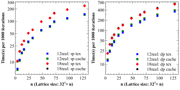
(b)

Figure 1: Time (s) per 1000 iterations. LABEL:sub@fig:time_32_3_ecc_off with ECC Off and LABEL:sub@fig:time_32_3_ecc_on with ECC On. sp: single precision, dp: double precision, 18real: full SU(3) matrix, 12real: 12 real parameterization, tex: using texture memory and cache: using L1 and L2 cache memory.

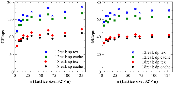
(a)

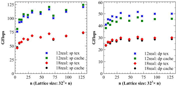
(b)

Figure 2: Performance in GFlops. LABEL:sub@fig:perf_32_3_ecc_off with ECC Off and LABEL:sub@fig:perf_32_3_ecc_on with ECC On. sp: single precision, dp: double precision, 18real: full SU(3) matrix, 12real: 12 real parameterization, tex: using texture memory and cache: using L1 and L2 cache memory.

For the GPU code the performance of the algorithm using a 12 parameter reconstruction and the full (18 number) representation in single and double precision was measured. Further, the GPU memory access using cache and texture memory was compared. We have also compared the performance of the three different ways to implement the 4D FFTs (1D FFTs, 3D plus 1D FFTs and 2D plus 2D FFTs) using a 12 parameter reconstruction and the full (18 number) representation in double precision, ECC off, L1 and L2 cache memory and texture memory for a $32^{4}$ lattice configuration with $\beta=6.0$. It turned out that using 2D plus 2D FFTs is 39-43% faster than using only 1D FFTs and 7-8% faster than using 3D plus 1D FFTs. The best performance for our 4D problem was achieved with 2D plus 2D FFTs using cufftPlanMany(). In the following, we will report on the results using such a type of decomposition for the GPU simulations.

For the run tests we generated a number of $32^{3}\times n$ gauge configurations at $\beta=6.2$. In Figs. 1 and 2 we show the outcome of the simulation when using the GPU and compare the effects of switching from single precision to double precision. The change in precision leads to a decrease in performance when going to double precision by a factor which can be $2.5$. The maximum of the performance code was 186 GFlops for a run in single precision with 12 parameter reconstruction using the texture memory. It was observed that using texture memory instead of L1 and L2 cache memory produced always a better performance. Turning on or off ECC also leads to differences in performance around 1.6 - see Fig. 2.

The performance of the GPU code against the parallel implementation of the same algorithm using MPI is compared in Fig. 3 and Table 3 for a $32^{4}$ lattice volume and for $\beta=5.8,6.0$ and $6.2$ - see the caption of the figure and table for further details. The MPI scaling shows a good strong scaling with a linear speed-up against the number of computing nodes. The GPU code was clearly much faster than the MPI. The MPI implementation of the algorithm requires 32 Centaurus computing nodes, i.e. 256 CPU cores, to reproduce the performance of the GPU code.

$32^{4}$		GPU - 12 real		GPU - 18 real		CPU $-$ # nodes
$\beta$	iter.	Tex.	Cache	Tex.	Cache	8	4	2	1
5.8	10427	637.44	699.49	1049.42	1086.97	2512.31	4649.83	8157.63	16323.97
5.8	8772	536.31	588.49	882.80	914.36	2126.49	3927.31	6940.21	13766.01
5.8	5038	308.02	338.39	507.03	525.25	1219.21	2254.74	3919.44	7835.32
5.8	3806	232.67	255.34	383.02	396.76	916.74	1695.71	2962.78	5932.83
6.0	3286	200.87	220.57	330.71	342.57	792.92	1466.55	2570.43	5145.40
6.0	2954	180.65	198.17	297.29	307.93	719.52	1318.45	2309.70	4615.02
6.0	2320	141.84	155.73	233.50	241.86	561.31	1034.58	1823.44	3638.41
6.0	4189	256.31	281.04	421.65	436.64	1014.53	1877.51	3276.73	6582.08
6.2	1083	66.42	72.69	109.00	112.92	263.78	484.91	849.60	1690.28
6.2	1342	82.06	90.07	135.07	139.92	325.81	600.56	1046.26	2087.11
6.2	5403	330.33	362.54	543.83	563.19	1307.71	2403.98	4201.31	8462.38
6.2	765	46.78	51.35	77.01	79.77	185.05	342.56	599.99	1272.64

Table 3: Number of iterations and time (s) to perform Landau gauge fixing for a lattice volume of $32^{4}$ in double precision. This was done for three values of $\beta$ with four configurations each. The GPU code was tested in a Tesla C2070 GPU with ECC Off with and without the 12 parameter reconstruction for SU(3), the CPU code was tested in the Centaurus cluster, where each node has 8 computing cores and DDR Infiniband interconnecting the various nodes, using a full SU(3) matrix representation. The value of $\alpha$ is $0.08$ and the stop criterion is $\theta<1\times 10^{-15}$.

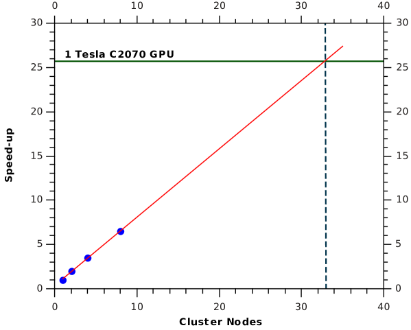
Figure 3: Strong scaling CPU tested for a $32^{4}$ lattice volume and comparison with the GPU for the best performance, 12 real number parameterization, ECC Off and using texture memory in double precision. In the Centaurus a cluster node means 8 computing cores.

5 Conclusion

We have compared the performance of the GPU implementation of the Fourier accelerated steepest descent Landau gauge fixing algorithm using CUDA with a standard MPI implementation built on the Chroma library. The run tests were done on $32^{4}$ and $\beta=5.8,6.0$ and $6.2$ pure gauge configurations, generated using the standard Wilson action.

In order to optimize the GPU code, its performance was investigated on $32^{3}\times n$ gauge configurations. The runs on a C2070 Tesla show that, for a 4D dimension lattice, the best performance was achieved with 2D plus 2D FFTs using cufftPlanMany() and using a 12 real parameter reconstruction with texture memory. From all the runs using a C2070 Tesla GPU, peak performance was measured as 186/71 GFlops for single/double precision. From the performance point of view, a run on a single GPU delivers the same performance as the CPU code when running on 32 nodes (256 cores), if one assumes a linear speed-up behavior.

As for the generation of gauge configurations, the use of GPUs reduces considerably the time of a simulation. At present, the main limitation of the GPUs both for gauge generation and for Landau gauge fixing is its limited memory size. For the Tesla C2070, the memory is 6GB. This allows us to consider lattice volumes up to $56^{4}$ using 12 real number parameterization in double precision to perform gauge fixing on a single GPU. In order to consider larger lattice volumes on GPU architectures, one has to consider a multi-GPU implementation. We leave this for future work.

References

- [1] S. Elitzur, Impossibility of Spontaneously Breaking Local Symmetries, Phys.Rev. D12 (1975) 3978–3982. doi:10.1103/PhysRevD.12.3978.
- [2] G. Martinelli, C. Pittori, C. T. Sachrajda, M. Testa, A. Vladikas, A General method for nonperturbative renormalization of lattice operators, Nucl.Phys. B445 (1995) 81–108. arXiv:hep-lat/9411010, doi:10.1016/0550-3213(95)00126-D.
- [3] O. Oliveira, P. Silva, Exploring the infrared gluon and ghost propagators using large asymmetric lattices, Braz. J. Phys. 37 (2007) 201–207.
- [4] I. L. Bogolubsky, E. M. Ilgenfritz, M. Muller-Preussker, A. Sternbeck, Lattice gluodynamics computation of landau-gauge green’s functions in the deep infrared, Phys. Lett. B 676 (2009) 69.
- [5] O. Oliveira, P. Bicudo, Running Gluon Mass from Landau Gauge Lattice QCD Propagator, J.Phys.G G38 (2011) 045003. arXiv:1002.4151, doi:10.1088/0954-3899/38/4/045003.
- [6] P. O. Bowman, U. M. Heller, D. B. Leinweber, M. B. Parappilly, A. G. Williams, J. Zhang, Unquenched quark propagator in landau gauge, Phys. Rev. 71 (2005) 054507.
- [7] S. Furui, H. Nakajima, Unqueched kogut-susskind quark propagator in lattice landau gauge qcd, Phys. Rev. D 73 (2006) 074503.
- [8] P. Boucaud, F. D. Soto, J. P. Leroy, A. L. Yaouanc, Micheli, O. Pene, J. Rodriguez-Quintero, Ghost-gluon running coupling, power corrections, and the determination of , Phys. Rev. D79 (2009) 014508.
- [9] D. Dudal, O. Oliveira, N. Vandersickel, Indirect lattice evidence for the Refined Gribov-Zwanziger formalism and the gluon condensate in the Landau gauge, Phys.Rev. D81 (2010) 074505. arXiv:1002.2374, doi:10.1103/PhysRevD.81.074505.
- [10] L. Giusti, M. Paciello, C. Parrinello, S. Petrarca, B. Taglienti, Problems on lattice gauge fixing, Int.J.Mod.Phys. A16 (2001) 3487–3534. arXiv:hep-lat/0104012, doi:10.1142/S0217751X01004281.
- [11] C. Davies, G. Batrouni, G. Katz, A. S. Kronfeld, G. Lepage, et al., Fourier acceleration in lattice gauge theories. I. Landau gauge fixing, Phys.Rev. D37 (1988) 1581. doi:10.1103/PhysRevD.37.1581.
- [12] A. Cucchieri, T. Mendes, A multigrid implementation of the fourier acceleration method for landau gauge fixing, Phys. Rev. D57 (1998) 3811–3826.
- [13] A. Cucchieri, T. Mendes, 1. The Influence of Gribov copies on gluon and ghost propagators in Landau gauge. 2. A New implementation of the Fourier acceleration method, Nucl.Phys.Proc.Suppl. 63 (1998) 841–843. arXiv:hep-lat/9710040, doi:10.1016/S0920-5632(97)00917-1.
- [14] O. Oliveira, P. Silva, An Algorithm for Landau gauge fixing in lattice QCD, Comput.Phys.Commun. 158 (2004) 73–88. arXiv:hep-lat/0309184, doi:10.1016/j.cpc.2003.12.001.
- [15] R. G. Edwards, B. Joo, The Chroma software system for lattice QCD, Nucl. Phys. Proc. Suppl. 140 (2005) 832.
- [16] M. Pippig, PFFT - An extension of FFTW to Massively Parallel Architectures, Department of Mathematics, Chemnitz University of Technology, 09107 Chemnitz, Germany Preprint 06.
- [17] NVIDIA, NVIDIA CUDA C Programming Guide, version 4.1 Edition (2011).
- [18] N. Cardoso, P. Bicudo, Generating SU(Nc) pure gauge lattice QCD configurations on GPUs with CUDA and OpenMP arXiv:1112.4533.
- [19] NVIDIA, CUDA Toolkit 4.1 CUFFT Library (2012).
- [20] M. Schrock, The chirally improved quark propagator and restoration of chiral symmetry, Phys.Lett. B711 (2012) 217–224. arXiv:1112.5107.
- [21] M. Clark, R. Babich, K. Barros, R. Brower, C. Rebbi, Solving Lattice QCD systems of equations using mixed precision solvers on GPUs, Comput.Phys.Commun. 181 (2010) 1517–1528. arXiv:0911.3191, doi:10.1016/j.cpc.2010.05.002.
- [22] R. Babich, M. A. Clark, B. Joo, Parallelizing the QUDA Library for Multi-GPU Calculations in Lattice Quantum Chromodynamics arXiv:1011.0024.
- [23] M. Harris, Optimizing Parallel Reduction in CUDA, NVIDIA Developer Technology, NVIDIA GPU computing SDK, 3rd Edition (2010).
- [24] Portuguese Lattice QCD collaboration, http://nemea.ist.utl.pt/~ptqcd.