Time dependent action in $\phi^{6}$ potential

Abstract: The false vacuum decay in field theory from a coherently oscillating initial state is studied for $\phi^{6}$ potential. An oscillating bubble solution is obtained. The instantaneous bubble nucleation rate is calculated.

keywords: phase transition, tunneling, scalar field theory.

PACS numbers: 03.65.Sq, 04.62.1v

1 Introduction

Problems involving quantum mechanical tunneling in a time dependent setting may arise in a wide variety of contexts, such as Schwinger vacuum pair production for time-dependent laser pulses [1], pair creation of charged particles in time dependent background electromagnetic fields [2, 3, 4], quantum interference in vacuum pair production [5], Hawking radiation from black holes [6], spontaneous nucleation of topological defects in expanding universes [7] and false vacuum decay with time dependent initial states or time dependent potentials [8, 9].

Barrier penetration and tunneling for a particle moving in a one-dimensional potential are treated in all textbooks on quantum mechanics. The procedure is by making a WKB approximation and expanding the logarithm of the wave function in powers of $\hbar$. An alternative way to tunneling makes use of the Euclidean-path-integral (EPI) formulation of the theory [10]. According to Feynman [11], the amplitude for going from one state to another is given by the sum over all paths connecting the states weighted by ${\rm e}^{iS/\hbar}$, where $S$ is the action evaluated along the path. For classically allowed motion, the dominant contribution to the path corresponding to the solution of the real-time equation of motion. A convenient way to calculate the action is to switch to Euclidean time. In this case, the probability amplitude is ${\rm e}^{-S_{E}/\hbar}$, where $S_{E}$ is the difference of Euclidean actions between the instanton solution (instanton solution: the classical solution of the Euclidean equation of motion with appropriate boundary conditions) and false vacuum solution.

Most decay of the false-vacuum calculations in single scalar field theory make use of the EPI formalism. The Lagrangian of the theory is

$${\mathcal{L}}=\frac{1}{2}\partial_{\mu}\phi\partial_{\mu}\phi-V(\phi),$$

where $V(\phi)$ is a potential which has two nondegenerate minima: $\phi_{+}$ ($\phi_{-}$) is the false (true) vacuum. One begins by writing the Euclidean action and the equation of motion. The equations are solved to obtain the instanton solution with boundary conditions $\phi\rightarrow\phi_{+}$ for $\eta\rightarrow\infty$ and $\phi\simeq\phi_{-}$ for $\eta\rightarrow 0$, where $\eta=\sqrt{\tau^{2}+r^{2}}$ and $\tau$ is the Euclidean time. The instanton solution corresponds to a bubble being nucleated at $r=0$.

The bubble nucleation rate per unit time per unit volume is given by

$${\Gamma}=A\,{\rm e}^{-S_{E}/\hbar},$$

where $S_{E}$ is the difference of Euclidean action and $A$ is a constant. The relevant solution is the one which gives the least action. In flat space and at zero temperature, the dominant contribution comes from the unique O(4)-symmetric solution [12].

As pointed out in [8], EPI has several limitations. We are lost at the outset if $\phi$ couples to some external current or field which is time dependent. As an example of this case is a scalar field in a Friedmann-Robertson-Walker (FRW) cosmology, since the FRW space is a time dependent and cannot be written in static coordinates. Another example arises with the theories of two or more coupled field. Also, there is a limitation of EPI formalism in the theory of a single scalar field in flat space if the initial field configuration is more complicated than simply $\phi(\vec{x})=\phi_{+}$ or time-dependent potential. In this work we can consider the case where $\phi$ is homogenous and undergoing coherent oscillations about the false vacuum.

One approach to overcome these limitations is presented in [8]. The author studied the false-vacuum decay of a scalar field by making use of the functional Schrodinger equation. He studied the vacuum decay of a scalar field coupled to a time-dependent external field and derived the traversal time for bubble nucleation.

An alternative approach is presented in [9]. The authors presented a method based on WKB approximation combined with complex time path methods, which can be used to calculate the relevant tunneling probabilities. They applied their algorithm to production of charged particle-antiparticle pairs in a time-dependent electric field and false vacuum decay in field theory from a coherently oscillating initial state. For the field theory example, they considered the potential discussed in Coleman [10],

$$V(\phi)=\frac{\lambda}{2}(\phi^{2}-a^{2})^{2}+\frac{\epsilon}{2a}(\phi-a).$$

The influence of nontrivial background and decoherence on vacuum tunneling is presented in [13]. In this work we follow the algorithm presented in [9], and we discuss the effect of coherent oscillating false vacuum state on vacuum decay in the thin-wall approximation (TWA), but we choose the $\phi^{6}$ potential which was investigated by many authors in the context of condensed matter as well as particle physics (see for example [14, 15, 16, 17, 18, 19, 20, 21, 22, 23]). We have noticed that there is a large correction to the nucleation rate and the small oscillations about the false vacuum rendered the state more unstable.

The plan of this paper is as follows. In section $2$, the vacuum decay without oscillation about the false in TWA is discussed using Coleman’s approach. In section $3$, decay with oscillation about the false vacuum in the TWA is presented based on complex time method. In section $4$ the structure of the oscillating bubble is obtained, while in section $5$ bubble nucleation decay rate is calculated. Finally, the results are discussed.

2 Decay without oscillation about the false vacuum: Coleman’s approach

Let us consider a scalar field theory with a Lagrangian density

$${\mathcal{L}(\phi)}={1\over 2}~{}({\partial_{\mu}\phi})^{2}-V(\phi),$$

where the potential $V(\phi)$ is the effective potential at zero temperature and is given by

$$V(\phi)=g\phi^{6}-2g\lambda^{2}\phi^{4}+(g\lambda^{4}-\delta)\phi^{2},$$ (1)

we choose $g=0.07$ and $\lambda=2.39$. The potential is shown in Figure 1, it has two nondegenrate minima $\phi_{+}$(false vacuum) and $\phi_{-}$ (true vacuum) which are all independent of time.

Figure 1: The scalar field potential $V(\phi)$ with parameters: $g=0.07$, $\lambda=2.39$, and $\delta=0.2$.

Let us expand the true vacuum in powers of $\delta$

$$\phi_{-}=\lambda+e_{1}\delta+e_{2}\delta^{2}+...$$

To first order in $\delta$,

$$\phi_{-}=\lambda+\frac{1}{4g\lambda^{3}}\delta+\mathcal{O}(\delta^{2}),$$

$$V(\phi_{-})=-\delta\lambda^{2}+\mathcal{O}(\delta^{2})4$$

Similarly for the false vacuum

$$\phi_{+}=0+e_{1}\delta+e_{2}\delta^{2}+...,$$

and

$$\phi_{+}=0~{}{\rm for\,~{}all\,~{}orders~{}\,of\,}~{}\delta,$$

$$V(\phi_{+})=0~{}{\rm for\,~{}all\,~{}orders\,~{}of\,}~{}\delta$$

To calculate the probability of decay of the false vacuum in quantum field theory at zero temperature, one should first solve the Euclidean equation of motion of the instanton:

$$\partial_{\mu}\partial_{\mu}\phi={dV(\phi)\over d\phi},$$ (2)

with the boundary condition $\phi\to\phi_{+}$ as $\vec{x}^{2}+\tau^{2}\to\infty$ , where $\tau$ is the imaginary time. The probability of tunnelling per unit time per unit volume is given by

$$\Gamma=A~{}~{}e{{}^{-S_{E}[\phi]}},$$ (3)

where $S_{E}[\phi]$ is the Euclidean action corresponding to the solution of Eq. (2) and given by the following expression :

$$S_{E}[\phi]=\int d^{4}{x}\left[{1\over 2}\Big{(}{\partial\phi\over\partial\tau}\Big{)}^{2}+{1\over 2}\Big{(}\nabla\phi\Big{)}^{2}+V(\phi)\right].$$ (4)

Since we are interested in the lowest-action instanton, we can reduce the problem to one of one degree of freedom. If we assume O(4) rotational symmetry in Euclidean space, then an O(4) invariant solution of Eq. (2) exists and its action $S_{E}[\phi]$ will be lower than that of any O(4) noninvariant solution [12]. In this case Eq. (2) takes the simpler form

$${d^{2}\phi\over d\eta^{2}}+{3\over\eta}~{}{d\phi\over d\eta}={dV(\phi)\over d\phi},$$ (5)

where $\eta=\sqrt{\vec{x}^{2}+\tau^{2}}$, with boundary conditions

$$\mathrm{\phi\to\phi_{+}~{}~{}as}~{}~{}\eta\to\infty~{},~{}~{}{d\phi\over d\eta}=0~{}~{}\mathrm{at~{}~{}\eta=0}.$$

We denote the action of this solution by $S_{0}$. There is an interesting case (in the sense that the action can be calculated analytically) when

$$V(\phi_{+})-V(\phi_{-})=\lambda^{2}\delta+\mathcal{O}(\delta^{2})\equiv\rho_{0}$$ (6)

is much smaller than the height of the barrier. This is known as the thin-wall approximation (TWA) and the equation of motion (Eq. 5) becomes

$$\frac{d^{2}\phi}{d\eta^{2}}=\frac{dV(\phi)}{d\phi},$$ (7)

which can be solved analytically for some potentials. For the $\phi^{6}$ potential, the solution has the form [16, 17]

$$\phi^{2}_{\rm wall}(\eta)=\frac{\lambda^{2}}{1+{\rm e}^{\mu\eta}},$$ (8)

where $\mu=\sqrt{8g}\lambda^{2}$, and $\mu^{2}$ is the second derivative of the potential in the TWA limit evaluated at $\phi_{-}$.

The action $S_{0}$ of the O(4)-symmetric bubble is equal to

$$S_{0} = 2\pi^{2}\int_{0}^{\infty}d\eta~{}\eta^{3}~{}\left[{1\over 2}\Big{(}{d\phi\over d\eta}\Big{)}^{2}+V(\phi)\right]$$ (9)

$$= -{1\over 2}\pi^{2}\rho_{0}R_{0}^{4}+2\pi^{2}\sigma_{0}R_{0}^{3}.$$

Here $R_{0}$ is the radius of the bubble and $\sigma_{0}$ is the bubble wall surface energy (surface tension), which is given by

$$\sigma_{0} = \int_{0}^{\infty}d\eta\left[\Big{(}{d\phi\over d\eta}\Big{)}^{2}+g\,\phi^{2}(\phi^{2}-\lambda^{2})^{2}\right]$$ (10)

$$= -\int_{0}^{\lambda}d\phi\>\sqrt{2g\,\phi^{2}(\phi^{2}-\lambda^{2})^{2}}$$

$$= \frac{\sqrt{g}\lambda^{4}}{2\sqrt{2}},$$

and the integral should be calculated in the limit $\rho_{0}\to 0$.

The bubble radius $R_{0}$, is calculated by minimizing $S_{0}$, this gives us

$$R_{0}={{3\sigma_{0}}\over\rho_{0}},$$

whence it follows that

$$S_{0}={{27\pi^{2}\sigma_{0}^{4}}\over{2\rho_{0}^{3}}}.$$ (11)

The nucleation rate is then

$$\Gamma=A{\rm e}^{-S_{0}}=A{\rm e}^{-\frac{\pi^{2}}{6}\rho_{0}R_{0}^{4}}.$$ (12)

Another parameter which is defined to test the applicability of the TWA is the bubble wall thickness $L$ which must be much less than $R_{0}$ and is given by

$$L=\frac{1}{\mu}=\Bigg{(}\frac{d^{2}V(\phi_{-})}{d\phi^{2}}\Bigg{)}^{-1/2},$$ (13)

The same results can be obtained using the algorithm proposed in [9].

To summarize, in the TWA the instanton takes the following shape:

$$\phi(\eta)=\left\{\begin{array}[]{lll}\phi_{+}=\lambda+\mathcal{O}(\delta),&{\eta<<R~{}({\rm True~{}vacuum})}\\[5.69046pt] \phi_{\rm wall}(\eta)=\frac{\lambda^{2}}{1+{\rm e}^{\mu\eta}},&{\eta\sim R}\\[5.69046pt] \phi_{-}=0,&{\eta>>R~{}({\rm False~{}vacuum})}.\end{array}\right.$$ (14)

3 Decay with oscillation about the false vacuum: Complex time method

In this section we review the results obtained in [9]. We assume that the field is initially oscillating around the false vacuum $\phi_{f}$ and takes the form

$$\phi_{f}(t)=\phi_{+}+\alpha_{0}\,{\rm sin}\,\omega t.$$ (15)

Since the energy is conserved, then $E({\rm inside})+E({\rm wall})$ of the bubble must equal the energy present in the region before nucleation of the bubble: $E_{\rm initial}.$ Thus

$$E_{\rm bubble}({\rm inside})=\frac{4\pi}{3}V(\phi_{t})R^{3},$$

where $\phi_{t}$ is the true vacuum and the bubble wall has the energy

$$E_{\rm bubble}({\rm wall})=\frac{4\pi\sigma_{E}^{\rm bubble}R^{2}}{\sqrt{1-\dot{R}^{2}}},$$

where

$$\sigma_{E}^{\rm bubble}=\int_{\rm wall}dr\Bigg{[}\frac{1}{2}(\dot{\phi}_{\rm bubble})^{2}+\frac{1}{2}(\phi^{\prime}_{\rm bubble})^{2}+V(\phi_{\rm bubble})\Bigg{]}.$$

The initial energy from the false vacuum $\phi_{f}(t)$ has two contributions, namely

$$E_{\rm initial}({\rm inside})=\frac{4\pi}{3}R^{3}\Bigg{[}\frac{1}{2}(\dot{\phi}_{f}(t))^{2}+\frac{1}{2}(\phi^{\prime}_{f}(t))^{2}+V(\phi_{f}(t))\Bigg{]}=\frac{4\pi}{3}\rho_{E}^{\rm FV}R^{3},$$

and

$$E_{\rm initial}({\rm wall})=\frac{4\pi\sigma_{E}^{\rm FV}R^{2}}{\sqrt{1-\dot{R}^{2}}},$$

where

$$\sigma_{E}^{\rm FV}=\int_{\rm wall}dr\Bigg{[}\frac{1}{2}(\dot{\phi}_{f}(t))^{2}+V(\phi_{f}(t))\Bigg{]}.$$

From conservation of energy

$$E_{\rm bubble}({\rm inside})+E_{\rm bubble}({\rm wall})=E_{\rm initial}({\rm inside})+E_{\rm initial}({\rm wall})$$

which can be written as

$$\frac{4\pi\sigma_{E}R^{2}}{\sqrt{1-\dot{R}^{2}}}-\frac{4\pi}{3}\rho_{E}R^{3}=0,$$

with

$$\sigma_{E}=\sigma_{E}^{\rm bubble}-\sigma_{E}^{\rm FV},$$ (16)

and

$$\rho_{E}=\rho_{E}^{\rm FV}-V(\phi_{t}).$$ (17)

From the above two equations, we can define the radius of the bubble at some time $t_{0}$ as

$${\mathcal{R}_{0}}={3\sigma_{E}\over\rho_{E}},$$ (18)

and the radius at any later time $t$ (the trajectory) is

$$R(t)=\sqrt{{\mathcal{R}_{0}}^{2}+(t-t_{0})^{2}}.$$ (19)

The action ($S=S_{\rm bubble}-S_{\rm FV}$) is integrated over an imaginary time contour running from some initial time $t_{0}$ to $t_{0}+i{\mathcal{R}_{0}}$, where the bubble shrinks to zero size. The bubble action is given by

$$S_{\rm bubble}=-\int dt\Bigg{[}4\pi\sigma_{L}^{\rm bubble}(t)R^{2}(t)\sqrt{1-\dot{R}^{2}}+\frac{4\pi}{3}V(\phi_{t})R^{3}\Bigg{]},$$ (20)

where

$$\sigma_{L}^{\rm bubble} = -\int_{\rm wall}dr\Bigg{[}\frac{1}{2}\Big{(}\dot{\phi}_{\rm bubble}\Big{)}^{2}-\frac{1}{2}\Big{(}\phi^{\prime}_{\rm bubble}\Big{)}^{2}-V(\phi_{\rm bubble})\Bigg{]}$$

$$= \sigma_{E}^{\rm bubble}-\int_{\rm wall}dr\,\dot{\phi}^{2}_{\rm bubble}$$

while the false vacuum action is

$$S_{\rm FV}=-\int dt\Bigg{[}4\pi\sigma_{L}^{\rm FV}(t)R^{2}(t)\sqrt{1-\dot{R}^{2}}+\frac{4\pi}{3}\rho_{L}^{\rm FV}R^{3}\Bigg{]},$$ (21)

where

$$\sigma_{L}^{\rm FV}=\sigma_{E}^{\rm FV}-\int_{\rm wall}dr\,\dot{\phi}^{2}_{f}$$

and

$$\rho_{L}^{\rm FV}=\rho_{E}^{\rm FV}-\dot{\phi}^{2}_{f}$$

From Eqs. (20) and (21) the action is

$$S=-\int dt\Bigg{[}4\pi\sigma_{L}(t)R^{2}(t)\sqrt{1-\dot{R}^{2}}-\frac{4\pi}{3}\rho_{L}(t)R^{3}\Bigg{]},$$ (22)

where

$$\sigma_{L}(t)=\sigma_{E}-\int_{\rm wall}dr\,[\dot{\phi}^{2}_{\rm bubble}-\dot{\phi}^{2}_{f}],$$

$$\rho_{L}(t)=\rho_{E}-\dot{\phi}^{2}_{f}.$$

4 Structure of the Oscillating Bubble

We calculate the oscillating bubble $\phi_{\rm bubble}(r,t)$ for the $\phi^{6}$ potential which interpolates between the true vacuum $\phi_{t}$ and the false vacuum $\phi_{f}$. Since the initial state oscillates coherently then it breaks the symmetry of the theory from SO$(3,1)$ to SO$(3)$. Therefore, Eq. (2) becomes

$$\ddot{\phi}-\frac{1}{r^{2}}(r^{2}\phi^{\prime})^{\prime}=-\frac{dV}{d\phi}.$$ (23)

with the potential

$$V(\phi)=g\phi^{6}-2g\lambda^{2}\phi^{4}+(g\lambda^{4}-\delta)\phi^{2}.$$

Following [9], we will find a time-dependent solution $\phi_{\rm bubble}(r,t),$ which will be reduced to coherently oscillating field

$$\phi_{f}(t)=\phi_{+}+\alpha_{0}\,{\rm sin}\,\omega t$$ (24)

about the false vacuum as $r\rightarrow\infty.$ The frequency of the oscillations $(\omega)$ about the false vacuum is

$$\omega^{2}=\frac{d^{2}V}{d\phi^{2}}(\phi_{+})=2(g\lambda^{4}-\delta),$$

and its range is $0<\omega^{2}<4.57.$

We assumed the $\phi_{\rm bubble}(r,t)$ is a function of both space and time and takes the form

$$\phi_{\rm bubble}(r,t)=\phi_{0}(r)+\alpha(r)\,{\rm sin}\,\omega t.$$ (25)

After substituting Eq.(25) in Eq.(23) we get

$$\alpha^{\prime\prime}(r)+\frac{2}{r}\alpha^{\prime}(r)+\left[\omega^{2}-\frac{d^{2}V}{d\phi^{2}}(\phi_{0})\right]\alpha(r)=0.$$ (26)

Now we will solve the above equation of motion in three different regions.

Firstly, the region outside the bubble $(r>R)$. In this case, $\phi_{0}=\phi_{+}$ (false vacuum), $\frac{d^{2}V}{d\phi^{2}}(\phi_{0})\rightarrow\frac{d^{2}V}{d\phi^{2}}(\phi_{+})=\omega^{2}$, and Eq. (26) becomes

$$\alpha^{\prime\prime}(r)+\frac{2}{r}\alpha^{\prime}(r)=0,$$

which has a general solution

$$\alpha(r)=\frac{C}{r}+D.$$

As $r\to\infty$, $\alpha(r)=0$, hence $D=0$. At $r=R$, $\alpha(R)=C/R={\rm constant}$ which we set it equals to $\alpha_{0}$. So, in this region Eq. (25) becomes

$$\phi_{\rm bubble}(r,t)=\phi_{+}+\alpha_{0}\,{\rm sin}\,\omega t,$$

which is the same equation (24).

Secondly, the region inside the bubble $(r<R)$. Again, in this case, $\phi_{0}=\phi_{-}$ (true vacuum), $\frac{d^{2}V}{d\phi^{2}}(\phi_{0})\rightarrow\frac{d^{2}V}{d\phi^{2}}(\phi_{-})=\omega^{2}+k^{2}$, where $k^{2}=6g\lambda^{4}+18\delta$ and Eq. (26) becomes

$$\alpha^{\prime\prime}(r)+\frac{2}{r}\alpha^{\prime}(r)-k^{2}\alpha(r)=0,$$

which has a general solution

$$\alpha(r)=A\frac{{\rm sinh}kr}{kr}.$$

At $r=R$, $\alpha(r)=\alpha_{0}$ and $A=\alpha_{0}\frac{kR}{{\rm sinh}kR}.$ Hence

$$\alpha(r)=\alpha_{0}\frac{R}{r}\frac{{\rm sinh}kr}{{\rm sinh}kR}.$$

Note that when $\alpha(r)=0$, the oscillation decays to zero inside the bubble. Therefore, the thickness of this region ($\Delta$) is given by

$$\Delta=\frac{1}{\sqrt{6g\lambda^{4}+18\delta}}\simeq\frac{1}{\sqrt{18\delta}}$$

for small values of $\delta$. Since

$$kR\sim\frac{12\sigma_{0}}{\lambda^{2}\sqrt{\delta}}>>1,$$

then the solution for $\alpha(r)$ can be approximated to

$$\alpha(r)=\alpha_{0}\frac{R}{r}\frac{{\rm e}^{kr}-{\rm e}^{-kr}}{{\rm e}^{kR}-{\rm e}^{-kR}}\simeq\alpha_{0}\frac{R}{r}{\rm e}^{(r-R)/\Delta}$$ (27)

As pointed out in [9], there are three scales which characterizes the structure of the oscillating bubbles: the radius of the bubble $R\simeq 3\sigma_{0}/(\lambda^{2}\delta)$, the thickness of the bubble wall $L\simeq 1/\mu\simeq 1/\sqrt{\frac{d^{2}V}{d\phi^{2}}(\phi_{-})}\simeq 1/(\sqrt{8g}\lambda^{2})$ and the thickness of the region inside the bubble where the oscillations decay $\Delta\simeq 1/(\sqrt{18\delta})$ and they are related as $L<<\Delta<<R.$

Finally, the region near the wall $(r\sim R).$ In this case $\phi_{0}(r)=\phi_{\rm wall}(r)$ and it is computed when the potential is degenerate, i.e., when $\delta\rightarrow 0$ and is satisfying the differential equation

$$\frac{d^{2}\phi_{\rm wall}(r)}{dr^{2}}=\frac{dV}{d\phi}({\phi_{\rm wall}}),$$

which has a solution

$$\phi_{\rm wall}(r)=\frac{\lambda^{2}}{1+{\rm e}^{\mu r}},$$

where $\mu=V^{\prime\prime}(\phi_{-})=\sqrt{8g}\lambda^{2}$ up to a correction of first order in $\delta$ and it is the mass of excitations around the true vacuum. Since we are working within the frame of the TWA, we can neglect the term $\frac{2}{r}\alpha^{\prime}(r)$ in Eq. (26) and we approximate $\omega^{2}$ to $\omega^{2}\simeq 2g\lambda^{4}$. Then Eq. (26) becomes

$$\alpha^{\prime\prime}(r)+\left[\omega^{2}-\frac{d^{2}V}{d\phi^{2}}(\phi_{\rm wall}\right]\alpha(r)=0$$

which can be simplified to

$$\alpha^{\prime\prime}(r)+6g\lambda^{4}\left[\frac{4}{1+{\rm e}^{\mu(r-R)}}-\frac{5}{(1+{\rm e}^{\mu(r-R)})^{2}}\right]\alpha(r)=0$$

By assuming $x=\mu(r-R)$, then the above equation becomes

$$\alpha^{\prime\prime}(x)+\frac{3}{4}\left[\frac{4}{1+{\rm e}^{x}}-\frac{5}{(1+{\rm e}^{x})^{2}}\right]\alpha(x)=0.$$ (28)

We have solved the above equation numerically which is shown in Figure 2. One can interpolate the solution to an approximate function given by

$$\alpha(r)\simeq\frac{B}{4}\Bigg{[}0.013(\mu(r-R))^{2}+5.0\,{\rm tanh}^{2}0.15(\mu(r-R))-1.0\Bigg{]}$$ (29)

Since $\alpha(r)\to B$ in regions $r\leq R$, where we know that $\alpha(r)=\alpha_{0}$, we set $B=\alpha_{0}$.

Figure 2: The dots represents the numerical solution of Eq. (28) while the solid line as an approximate fit (Eq. (29)).

To summarize, we have found a solution for the oscillating bubble in the thin-wall approximation

$$\phi_{\rm bubble}(r,t)=\phi_{0}(r)+\alpha(r)\,{\rm sin}\,\omega t,$$ (30)

where $\phi_{0}(r)$ is the static solution given by Eq. (14), and $\alpha(r)$ is given by

$$\alpha(r)=\left\{\begin{array}[]{lll}\alpha_{0},&r\geq R+\frac{L}{2}\\[8.5359pt] \frac{\alpha_{0}}{4}\Big{[}0.013(\mu(r-R))^{2}+5.0\,{\rm tanh}^{2}0.15\mu(r-R)-1\Big{]},&R-\frac{L}{2}\leq r\leq R+\frac{L}{2}\\[8.5359pt] \alpha_{0}\frac{R}{r}{\rm e}^{(r-R)/\Delta},&r\leq R+\frac{L}{2}\end{array}\right.$$ (31)

5 Bubble Nucleation Decay Rate

The bubble nucleation rate per unit time per unit volume is given by

$$\Gamma=A\,{\rm e}^{-2{\rm Im}[S(t_{0})]}.$$ (32)

We need a time path which shrinks the bubble to zero size. As an example of a path is

$$R^{2}={\mathcal{R}_{0}^{2}}+(t-t_{0})^{2}$$

which yields to

$$t=t_{0}+i\sqrt{\mathcal{R}_{0}^{2}-R^{2}},~{}~{}{\rm for}~{}R<\mathcal{R}_{0}.$$

We divide the action in Eq. (22) into two parts:

$$S_{1}=-\int_{t_{0}+i\mathcal{R}_{0}}^{t_{0}}dt\left[4\pi\sigma_{E}R^{2}\sqrt{1-\dot{R}^{2}}-\frac{4\pi}{3}\rho_{E}R^{3}\right]$$ (33)

and

$$S_{2}=-\int_{t_{0}+i\mathcal{R}_{0}}^{t_{0}}dt\left[4\pi R^{2}\sqrt{1-\dot{R}^{2}}\int_{R-\frac{L}{2}}^{R+\frac{L}{2}}dr(\dot{\phi}^{2}_{\rm bubble}-\dot{\phi}_{f}^{2})-\frac{4\pi}{3}R^{3}\dot{\phi}^{2}_{t}\right]$$ (34)

For the first part $S_{1}$, the calculations proceed as in the static case as shown in section $2$. The result is:

$${\rm Im}S_{1}=\frac{\pi^{2}}{12}\rho_{E}\mathcal{R}_{0}^{4}$$ (35)

where $\rho_{E}$ is the energy density and is given by:

$$\rho_{E} = \rho_{E}^{\rm FV}-V(\phi_{t})$$

$$= \frac{1}{2}[\dot{\phi}_{f}(t)]^{2}+V(\phi_{f})-V(\phi_{t})=\rho_{0}+\frac{1}{2}\alpha_{0}^{2}\omega^{2},$$

which is time independent. Note that the oscillation about the false vacuum increases the energy density and in the limit $\alpha_{0}\to 0$, $\rho_{E}=\rho_{0}$ as expected.

The surface tension $\sigma_{E}$ is given by

$$\sigma_{E}=\sigma_{E}^{\rm bubble}-\sigma_{E}^{\rm FV},$$

where $\sigma_{E}^{\rm bubble}$ is given by

$$\sigma_{E}^{\rm bubble}=\int_{\rm wall}dr\left[\frac{1}{2}\left(\dot{\phi}_{\rm bubble}(r,t)\right)^{2}+\frac{1}{2}\left(\phi^{\prime}_{\rm bubble}(r,t)\right)^{2}+V(\phi_{\rm bubble}).\right]$$

Using

$$\phi_{\rm bubble}(r,t)=\phi_{0}(r)+\alpha(r)\,{\rm sin}\,\omega t=\phi_{0}(r)+\beta(r,t)$$

and

$$V(\phi_{\rm bubble})=V(\phi_{0})+\beta(r,t)\frac{dV}{d\phi}(\phi_{0})+\frac{1}{2}\beta^{2}(r,t)\frac{d^{2}V}{d\phi^{2}}(\phi_{0})$$

then

$$\sigma_{E}^{\rm bubble} = \int_{\rm wall}dr\Bigg{[}\frac{1}{2}\omega^{2}\alpha^{2}(r){\rm cos}^{2}\,\omega t+\frac{1}{2}\phi^{{}^{\prime}2}_{0}(r)+\frac{1}{2}\beta^{{}^{\prime}2}(r,t)+\phi_{0}^{\prime}(r)\beta^{\prime}(r,t)+V(\phi_{0})$$

$$+ \beta(r,t)\frac{dV}{d\phi}(\phi_{0})+\frac{1}{2}\beta^{2}(r,t)\frac{d^{2}V}{d\phi^{2}}(\phi_{0})\Bigg{]}$$

$$= \sigma_{0}+\sigma_{1}+\sigma_{2},$$

where

$$\sigma_{0}=\int_{\rm wall}dr\Big{[}\frac{1}{2}\phi^{{}^{\prime}2}_{0}(r)+V(\phi_{0})\Big{]},$$

and

$$\sigma_{1}=\int_{\rm wall}dr\Big{[}\phi_{0}^{\prime}(r)\beta^{\prime}(r,t)+\beta(r,t)\frac{dV}{d\phi}(\phi_{0})\Big{]},$$

which can be shown equals to zero. While

$$\sigma_{2} = \int_{\rm wall}dr\Big{[}-\frac{1}{2}\omega^{2}\alpha^{2}(r){\rm sin}^{2}\,\omega t+\frac{1}{2}\alpha^{\prime 2}(r){\rm sin}^{2}\,\omega t+\frac{1}{2}\beta^{2}(r,t)\frac{d^{2}V}{d\phi^{2}}(\phi_{0})+\frac{1}{2}\omega^{2}\alpha^{2}\Big{]}$$

$$= \int_{\rm wall}dr\frac{1}{2}\Bigg{[}\Bigg{(}\alpha^{2}(r)\Big{(}\frac{d^{2}V}{d\phi^{2}}(\phi_{0})-\omega^{2}\Big{)}+\alpha^{\prime 2}(r)\Bigg{)}{\rm sin}^{2}\omega t+\omega^{2}\alpha^{2}(r)\Bigg{]}$$

$$= \int_{\rm wall}dr\frac{1}{2}\Bigg{[}\Bigg{(}\alpha(r)\alpha^{\prime\prime}(r)+(\alpha^{\prime}(r))^{2}\Bigg{)}{\rm sin}\,^{2}\omega t+\omega^{2}\alpha^{2}(r)\Bigg{]}$$

$$= \frac{1}{2}\omega^{2}\int_{\rm wall}dr\alpha^{2}(r)=0.06\frac{\omega^{2}}{2}L\alpha_{0}^{2}$$

Therefore,

$$\sigma_{E}^{\rm bubble}=\sigma_{0}+0.06\frac{\omega^{2}}{2}\alpha_{0}^{2}L$$

while the value surface density due to the false vacuum is

$$\sigma_{E}^{\rm FV}=\int_{\rm wall}dr\Big{[}\frac{1}{2}\dot{\phi}_{f}^{2}(r,t)+V(\phi_{f})\Big{]}=\frac{1}{2}\alpha_{0}^{2}\omega^{2}\int_{R-\frac{L}{2}}^{R+\frac{L}{2}}dr=\frac{1}{2}\alpha_{0}^{2}\omega^{2}L$$

Hence,

$$\sigma_{E}=\sigma_{0}-0.47\omega^{2}\alpha_{0}^{2}L$$ (36)

which is again independent of time, but the oscillation decreases its value and in the limit $\alpha_{0}\to 0$, $\sigma_{E}=\sigma_{0}$ as expected. Moreover, notice that $\sigma_{E}$ equals to zero when $\alpha_{0}^{2}=\sigma_{0}/(0.47\omega^{2}L).$ We would like to see the effect of $\alpha$ on the radius of the bubble. Figure $3$ shows the ratio of the relative difference of the radius of the bubble with oscillation about the false vacuum ($\mathcal{R}$) and radius without oscillation ($R_{0}$) versus $\alpha_{0}$. We notice from the figure that at $\alpha_{0}=0$ the value of $\mathcal{R}$ equals to $R_{0}$ and at $\alpha_{0}=2.57$ its value is zero for $\delta=0.2$. So, the allowed value of $\alpha_{0}$ is $0<\alpha_{0}<2.57$.

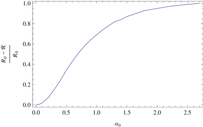
Figure 3: The ratio of the relative difference of the radius of the bubble with oscillation about the false vacuum and radius without oscillation versus $\alpha_{0}$.

The second part of the action $S_{2}$ is given by

$$S_{2} = -\int_{t_{0}+i\mathcal{R}_{0}}^{t_{0}}dt\Bigg{[}4\pi R^{2}(t)\sqrt{1-\dot{R}^{2}(t)}\int_{\rm wall}dr\Big{(}\dot{\phi}_{\rm bubble}^{2}(r,t)-\dot{\phi}_{f}^{2}(r,t)\Big{)}-\frac{4\pi}{3}R^{3}(t)\dot{\phi}_{f}^{2}(r,t)\Bigg{]}$$

$$= -4\pi\omega^{2}\alpha_{0}^{2}\int_{t_{0}+i\mathcal{R}_{0}}^{t_{0}}dt\Bigg{[}LDR^{2}(t)\sqrt{1-\dot{R}(t)^{2}}-\frac{1}{3}R^{3}(t)\Bigg{]}{\rm cos}^{2}\omega t$$

where $D=-0.94$. Using $R(t)=\sqrt{\mathcal{R}_{0}^{2}+(t-t_{0})^{2}}$ and $t-t_{0}={\mathcal{R}_{0}}zi$, then

$$S_{2} = -4\pi\omega^{2}\alpha_{0}^{2}\Bigg{[}\frac{i}{2}{\mathcal{R}_{0}}\int_{1}^{0}dz\left(LD{\mathcal{R}_{0}^{2}}\sqrt{1-z^{2}}-\frac{1}{3}{\mathcal{R}_{0}^{3}}(1-z^{2})^{\frac{3}{2}}\right)$$

$$+ i{\mathcal{R}_{0}}\int_{1}^{0}dzLD{\mathcal{R}_{0}^{2}}\sqrt{1-z^{2}}\frac{1}{4}\Big{(}{\rm e}^{2i\omega t_{0}}{\rm e}^{-2\omega{\mathcal{R}_{0}}z}+{\rm e}^{-2i\omega t_{0}}{\rm e}^{2\omega{\mathcal{R}_{0}}z}\Big{)}$$

$$+ i{\mathcal{R}_{0}}\int_{1}^{0}dz\Big{(}-\frac{1}{3}{\mathcal{R}_{0}^{3}}(1-z^{2})^{\frac{3}{2}}\Big{)}\frac{1}{4}\Big{(}{\rm e}^{2i\omega t_{0}}{\rm e}^{-2\omega{\mathcal{R}_{0}}z}+{\rm e}^{-2i\omega t_{0}}{\rm e}^{2\omega{\mathcal{R}_{0}}z}\Big{)}\Bigg{]}$$

$$= -4\pi\omega^{2}\alpha_{0}^{2}(I_{1}+I_{2}+I_{3})$$

It can be easily shown that

$${{\rm Im}I_{1}} = \frac{1}{2}{\mathcal{R}_{0}}\int_{1}^{0}dz\Bigg{[}LD{\mathcal{R}_{0}^{2}}\sqrt{1-z^{2}}-\frac{1}{3}{\mathcal{R}_{0}^{3}}(1-z^{2})^{\frac{3}{2}}\Bigg{]}$$

$$= \frac{\pi}{16\omega}(0.94){\mathcal{R}_{0}^{3}}+\frac{\pi}{32}\mathcal{R}_{0}^{4}.$$

and

$${\rm Im}I_{2} = {\mathcal{R}_{0}^{3}}DL\int_{1}^{0}dz\sqrt{1-z^{2}}\frac{1}{4}\Big{(}{\rm cos}\,2\omega t_{0}\Big{)}\Big{(}{\rm e}^{-2\omega{\mathcal{R}_{0}}z}+{\rm e}^{2\omega{\mathcal{R}_{0}}z}\Big{)}$$

$$= -{\mathcal{R}_{0}^{3}}DL\frac{1}{4}\Big{(}{\rm cos}\,2\omega t_{0}\Big{)}\int_{-1}^{1}dz\sqrt{1-z^{2}}{\rm e}^{2\omega{\mathcal{R}_{0}}z}$$

$$= -\frac{D}{2\omega}\frac{{\mathcal{R}_{0}^{3}}}{4}\frac{\pi}{2\omega\mathcal{R}_{0}}\Big{(}{\rm cos}\,2\omega t_{0}\Big{)}I_{1}(2\omega\mathcal{R}_{0})$$

by using Modified Bessel Functions

$$I_{\nu}(z)=\frac{(z/2)^{\nu}}{\sqrt{\pi}\Gamma(\nu+1/2)}\int_{-1}^{1}(1-t^{2})^{\nu-1/2}{\rm e}^{\pm zt}dt$$

and $L\simeq 1/\sqrt{8g\lambda^{2}}\simeq 1/(2\omega)$. Similarly for $I_{3}$,

$${\rm Im}I_{3} = \frac{\mathcal{R}_{0}^{4}}{3}\frac{1}{4}\Big{(}{\rm cos}\,2\omega t_{0}\Big{)}\int_{-1}^{1}dz({1-z^{2}})^{3/2}{\rm e}^{2\omega{\mathcal{R}_{0}}z}$$

$$= \frac{1}{16}\pi{\mathcal{R}_{0}^{2}}\frac{1}{\omega^{2}}\Big{(}{\rm cos}\,2\omega t_{0}\Big{)}I_{2}(2\omega\mathcal{R}_{0}).$$

Therefore,

$${\rm Im}S_{2} = \pi^{2}{\mathcal{R}_{0}^{2}}\alpha_{0}^{2}\Bigg{(}\Big{(}\frac{0.94}{8}\Big{)}(2\omega\mathcal{R}_{0})+\frac{(2\omega\mathcal{R}_{0})^{2}}{32}$$ (37)

$$+ \Bigg{(}(\frac{0.94}{4})I_{1}(2\omega\mathcal{R}_{0})+\frac{1}{4}I_{2}(2\omega\mathcal{R}_{0})\Bigg{)}{\rm cos}\,2\omega t_{0}\Bigg{)}$$

The total instantaneous bubble nucleation rate is then

$$\Gamma(t_{0}) = {\rm Exp}\Bigg{[}-\frac{\pi^{2}}{6}\rho_{E}\mathcal{R}_{0}^{4}-\pi^{2}{\mathcal{R}_{0}^{2}}\alpha_{0}^{2}\Bigg{(}\Big{(}\frac{3.76}{32}\Big{)}(2\omega\mathcal{R}_{0})+\Big{(}\frac{1}{32}\Big{)}(2\omega\mathcal{R}_{0})^{2}$$ (38)

$$+ \Bigg{(}(\frac{0.94}{4})I_{1}(2\omega\mathcal{R}_{0})+\frac{1}{4}I_{2}(2\omega\mathcal{R}_{0})\Bigg{)}{\rm cos}\,2\omega t_{0}\Bigg{)}\Bigg{]}.$$

By fixing the value of $\delta$ to $0.2$, we have shown that total action of the instanton (${\rm Im}S$) varies with $\alpha_{0}$. It has a maximum value ($S_{\rm max.}$) at $\alpha_{0}\approx 0.12$, if we assume ${\rm cos}\,2\omega t_{0}=1$. Figure $4$ shows a plot of ($(S-S_{0})/S_{\rm max}$) versus $\alpha_{0}$ where $S_{0}$ is the action give by Eq. (11). At $\alpha_{0}=0$, we have $S=S_{0}$ while at $\alpha_{0}\approx 0.12$, most contribution of the action comes from the oscillatory part $\omega\mathcal{R}_{0}$ when it has its maximum value. For $\alpha_{0}>0.12$, the contribution from the oscillatory part starts decreasing and the total action converges to $S_{0}$ for higher values of $\alpha_{0}$. So, we conclude that the effect of oscillation about the false vacuum has a significant contribution to the tunneling for small specific value of $\alpha_{0}$.

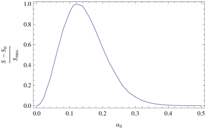
Figure 4: The plot of ($(S-S_{0})/S_{\rm max}$) versus $\alpha_{0}$.

6 Conclusion

In this paper we have discussed the problem of false vacuum decay in field theory, where the initial state consists of coherent field oscillations about the false vacuum for $\phi^{6}$ potential. We have shown that there is an upper limit for the amplitude of the oscillation of the field about the false vacuum. Moreover, The effect of oscillation about the false vacuum has a significant contribution to the tunneling for small specific values of the amplitude. The method we have used is based on the WKB approximation and the solutions of classical equation of motion of the instanton along complex time contour. We obtained a time-dependent decay rate in the case of small oscillations.

The importance of our work is for cosmological models which are based on quantum tunneling, for example: eternal inflation [24], the Hartle-Hakwing-instanton [25], the Hawking-Moss instanton [26], the quantum creation of topological defects, e.g. strings and branes in a fixed space-time [27]. Moreover, several authors have suggested that string theory in four dimensions might have many different vacua [28], which are all represent local minima and the tunneling between different local minima is of great importance. Finally, we would like to mention here that an important problem which can be investigated is the quantum nucleation of cosmic strings and domain walls in an expanding universe.

References

[1] Cesim K. Dumlu, Gerald V. Dunne, Phys.Rev. D83 (2011)
065028.
Cesim K. Dumlu, Gerald V. Dunne,
Phys.Rev.Lett. 104 (2010) 250402.
[2] E. Brezin and C. Itzykson, Phys. Rev. D 2 (1970) 1191.
[3] M. S. Marinov and
V. S. Popov, Fortschr. Phys. 25 (1977) 373.
[4] J. Audretsch, J. Phys. A 12 (1979) 1189.
[5] Cesim K. Dumlu, Gerald V. Dunne,
Phys.Rev. D 84 (2011) 125023.