Z(2) Gauge Neural Network and its Phase Structure

Abstract

We study general phase structures of neural-network models that have Z(2) local gauge symmetry. The Z(2) spin variable $S_{i}=\pm 1$ on the $i$-th site describes a neuron state as in the Hopfield model, and the Z(2) gauge variable $J_{ij}=\pm 1$ describes a state of the synaptic connection between $j$-th and $i$-th neurons. The gauge symmetry allows for a self-coupling energy among $J_{ij}$’s such as $J_{ij}J_{jk}J_{ki}$, which describes reverberation of signals. Explicitly, we consider the three models; (I) annealed model with full and partial connections of $J_{ij}$, (II) quenched model with full connections where $J_{ij}$ is treated as a slow quenched variable, and (III) quenched three-dimensional lattice model with the nearest-neighbor connections. By numerical simulations, we examine their phase structures paying attention to the effect of reverberation term, and compare them each other and with the annealed 3D lattice model which has been studied beforehand. By noting the dependence of thermodynamic quantities upon the total number of sites and the connectivity among sites, we obtain a coherent interpretation to understand these results. Among other things, we find that the Higgs phase of the annealed model is separated into two stable spin-glass phases in the quenched cases (II) and (III).

Keywords: neural network; lattice gauge theory; phase structure

1 Introduction

Although it is just a collection of neurons and other biological cells, the human brain exhibits quite various functions such as learning patterns and recalling them. We are still in a way to obtain a physical understanding of these functions in a comprehensive manner. As a well-known and convincing step on this way, one may refer to the Hopfield model[1] for explanation of associative memory. Here, the state of $i$-th neuron is described simply by a Z(2) variable as $S_{i}=1$(excited), -1(unexcited). This model is a good example of a simple physical model that describes essential mechanism of some functions of the human brain.

Concerning to the learning process, many models have been proposed and studied[2]. In Ref.[3, 4], the Z(2) gauge model is introduced as a model of learning, where the state of synaptic connections from the $j$-th neuron to the $i$-th neuron is described by the gauge variable $J_{ij}=1$(excitatory connection) and -1(inhibitory connection). The plasticity of $J_{ij}$ is described by the equation of motion which basically decreases the gauge-invariant energy subject to fluctuations caused by random noises. The reason why the local gauge symmetry is implemented there is two fold;

(i) There is a freedom to assign two physical neuron states(excited and unexcited) to a two-valued local variable $S_{i}=\pm 1$ (See Ref.[4] for more details).

(ii) In the real human brain, electric signals are transfered according to the rule of electromagnetism which is based on the U(1) local gauge symmetry. Because Z(2) is a subgroup of U(1) group, the Z(2) gauge symmetry may be viewed as a remnant of this U(1) symmetry.

A by-product of the gauge symmetry is that the time evolution of $J_{ij}$ automatically involves a term suggested by Hebb’s law[6], $J_{ij}(t+\Delta t)-J_{ij}(t)\propto S_{i}S_{j}+\cdots$[4].

In Ref.[4] we introduced a simple Z(2) gauge model defined on the three-dimensional (3D) lattice and studied its various aspects such as the phase structure, ability of learning and recalling patterns, etc. We obtained some interesting results such as an existence of confinement phase in which neither learning and recalling is possible.

Although these results warrant that the Z(2) gauge neural network is worth further studies, the 3D lattice model has some flaws as a model of the human-brain functions. For example, (i) its nearest-neighbor connections of the 3D lattice model are too scarce compared with those of the human brain, and (ii) treating $S_{i}$ and $J_{ij}$ on an equal footing in the time evolution is not realistic because, in the human brain, the rate of time variation of synaptic strength is much slower than that of neuron state. One certainly needs to incorporate ample synaptic connections and different scales in time evolution of variables.

In this paper we consider various models of Z(2) gauge neural network respecting these two points, and study their properties numerically. Comparison of these results with those of the above 3D lattice model[3, 4] provides us with more understanding of the general properties of the Z(2) gauge network and relevance of Z(2) gauge symmetry to modeling the human brain. In particular, we consider certain quenched models in which the synaptic variables are treated as slow-varying quenched variables, and find that there appear spin-glass (SG) states.

The paper is organized as follows: In Sect.2 we explains the explicit models (I-III) in detail. In Sect.3-5 we present the results of Monte Carlo (MC) simulations for the phase structure of each model. In Sect.6 we present conclusions and discussions. In Appendices A-E some technical topics are studied.

2 Z(2) Gauge Models

In this section we introduce the Z(2) gauge models, Model I-III, that we shall study. They are classified by the following two points;

(a) magnitude of connectivity of synaptic connections; full and partial connections or the nearest-neighbor connections on the 3D lattice,

(b) nature of synaptic variables; annealed one ($J_{ij}$ varies in a similar time-scale as $S_{i}$) or quenched one ($J_{ij}$ varies much slower than $S_{i}$).

These models are listed in Table 1 together with the 3D annealed lattice model which we call Model 0. We note here that Models 0 and III are put on the 3D lattice where neurons reside on lattice sites, and therefore the distance between a pair of neurons can be defined. In contrast, Models II and III have full (or partial) connections and there are no concepts of distance between neurons as long as one does not introduce explicitly a metric space in which neurons reside.

	model	connections	synaptic variables
0	3D lattice/anneal	3D lattice	anneal
I	full/anneal	full and partial	anneal
II	full/quench	full	quench
III	3D lattice/quench	3D lattice	quench

Table 1. List of Z(2) gauge models classified by connections and treatment of synaptic variables: Model 0 studied in Ref.[4] and Models I-III studied in the present paper.

2.1 Model 0: Annealed 3D Lattice Model

Before going to Models I-III, let us review Model 0 and its results[4] briefly. The energy $E_{0}$ of Model 0 is given by[5]

$$E_{0} = -c_{1}\sum_{x}\sum_{\mu}S_{x+\mu}J_{x\mu}S_{x}-c_{2}\sum_{x}\sum_{\mu>\nu}J_{x\mu}J_{x+\mu,\nu}J_{x+\nu,\mu}J_{x\nu}.$$ (2.1)

$S_{x}(=\pm 1)$ is the neuron variable ($S_{i}$) put on the site $x$ of the 3D lattice and $J_{x\mu}(=\pm 1)$ is the synaptic variable ($J_{ij}$) put on the link $(x,x+\mu)$ connecting nearest-neighbor sites, where $\mu=1,2,3$ is the direction index as well as the unit vector in that direction. $c_{1}$ and $c_{2}$ are real parameters. The $c_{1}$-term, the Hopfield energy[1], describes the process of signals transferring from the neuron at $x$ to the neuron at $x+\mu$ (and vice versa), and the $c_{2}$-term describes the process of signals running around the contour $(x,x+\mu,x+\mu+\nu,x+\nu)$ (and the reversed one) as a reverberating circuit[6, 7]. This $c_{2}$-term also corresponds to the magnetic energy in the U(1) gauge theory[8].

$E_{0}$ is invariant under the Z(2) gauge transformation,

$$S_{x}\rightarrow S_{x}^{{}^{\prime}}\equiv V_{x}S_{x},\ \ J_{x\mu}\rightarrow J_{x\mu}^{{}^{\prime}}\equiv V_{x+\mu}J_{x\mu}V_{x},\ \ V_{x} = \pm 1,$$ (2.2)

due to $V_{x}^{2}=1$.

We introduce the fictitious temperature $T$ as a parameter to control the fluctuations of $S_{x}$ and $J_{x\mu}$. The partition function at $T$ is given by

$$Z_{0} = \sum_{S}\sum_{J}\exp(-E_{0}),$$

$$\sum_{S} \equiv \prod_{x}\sum_{S_{x}=\pm 1},\ \sum_{J}\equiv\prod_{x}\prod_{\mu}\sum_{J_{x\mu}=\pm 1},$$ (2.3)

where we have included the inverse temperature $\beta\equiv 1/T$ into the coefficients $c_{1}$ and $c_{2}$ ($c_{i}$ is proportional to $\beta$). The average $\langle O(S,J)\rangle$ of a function $O(S,J)$ w.r.t. $Z_{0}$ is given by

$$\langle O(S,J)\rangle = \frac{1}{Z_{0}}\sum_{S}\sum_{J}\ O(S,J)\exp(-E_{0}).$$ (2.4)

The phase diagram in the $c_{2}$-$c_{1}$ plane is given in Fig.1. There are three phases as listed in Table.2, where the order parameters of the mean-field theory (MFT) and the ability of learning and recalling patterns are also given. The order of transition is of first-order for the confinement-Higgs transition, while it is of second-order for the confinement-Coulomb transition and for the Coulomb-Higgs transition[9].

phase	$\langle J_{x\mu}\rangle$	$\langle S_{x}\rangle$	ability
Higgs	$\neq 0$	$\neq 0$	learning and recalling
Coulomb	$\neq 0$	$0$	learning
confinement	$0$	$0$	N.A.

Table2. Phases, order parameters of the mean-field theory[10], and ability of learning and recalling patterns in the 3D Z(2) lattice gauge model, Model 0 of (2.3) (See Ref.[4]). The names for three phases are those used in lattice gauge theory[8].

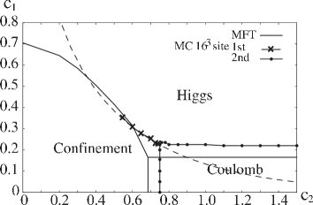
Figure 1: Phase structure of the 3D Z(2) lattice gauge model, Model 0 of (2.3), in the $c_{2}$-$c_{1}$ plane (taken from Ref.[4]). The crosses and filled squares denote first and second-order transitions respectively. The real curves are the result of MFT, and the dashed curve is the self-dual curve on which a part of phase transition points may locate.

2.2 Model I: Annealed Model with full and partial connections

The annealed model with full and partial connections involves $N$ neurons. The state of the neuron at the $i$-th site ($i=1,\cdots,N$) is described by the neuron variable $S_{i}(=\pm 1)$, and the state of synaptic connection connecting $j$-th neuron and $i$-th neuron is described by the synaptic variable $J_{ij}(=\pm 1)$. In this paper we consider the case of symmetric coupling, $J_{ij}=J_{ji}$, and only $J_{ij}$ with $i<j$ are independent[11]. The total number of independent variables of $J_{ij}$ is $N_{\rm l}\equiv{}_{N}C_{2}=N(N-1)/2$. We also have the connection parameter $\epsilon_{ij}$,

$$\epsilon_{ij}=\left\{\begin{array}[]{ll}1&{\rm connected},\\ 0&{\rm disconnected}.\end{array}\right.$$ (2.7)

The energy $E_{\rm I}(\epsilon)$ for a fixed configuration of connections, $\epsilon\equiv\{\epsilon_{ij}\}$, is given by

$$E_{\rm I}(\epsilon) = -c_{1}\sum_{i<j}\epsilon_{ij}S_{i}J_{ij}S_{j}-\frac{c_{2}}{N}\sum_{i<j<k}\epsilon_{ij}\epsilon_{jk}\epsilon_{ki}J_{ij}J_{jk}J_{ki}.$$ (2.8)

Each term is depicted in Fig.2. It may be viewed as a direct extension of the energy (2.1) of Model 0. We note that the $c_{2}$-term for reverberation consists of the product of three $J$’s in contrast to the product of four $J$’s in the 3D model, Model 0, reflecting the difference of the minimum number of $J$’s to construct nontrivial (not a constant) gauge-invariant term. We have introduced the factor $N^{-1}$ in the coefficient of the $c_{2}$-term for later convenience. One may include other gauge-invariant terms to the energy, such as $c_{4}J_{ij}J_{jk}J_{kl}J_{li}$, but the properties of the “minimum” form (2.8) should be studied first. $E_{\rm I}(\epsilon)$ is invariant under Z(2) gauge transformation similar to (2.2),

$$S_{i}\rightarrow S_{i}^{{}^{\prime}}\equiv V_{i}S_{i},\ \ J_{ij}\rightarrow J_{ij}^{{}^{\prime}}\equiv V_{i}J_{ij}V_{j},\ \ V_{i}=\pm 1.$$ (2.9)

Figure 2: Each term of the energy $E_{\rm I}(\epsilon)$ of (2.8) of Model I for the case $\epsilon_{ij}=\epsilon_{jk}=\epsilon_{ki}=1$. The filled circle denotes $S_{i}$ and the segment denotes $J_{ij}$.

The partition function $Z_{\rm I}(\epsilon)$ for a fixed configuration $\epsilon$ and the average $\langle O\rangle_{\epsilon}$ over $Z_{\rm I}(\epsilon)$ are given by

$$Z_{\rm I}(\epsilon) = \sum_{S}\sum_{J}\exp\left(-E_{\rm I}(\epsilon)\right),$$

$$\langle O\rangle_{\epsilon} = \frac{1}{Z_{\rm I}(\epsilon)}\sum_{S}\sum_{J}O(S,J)\exp\left(-E_{\rm I}(\epsilon)\right),$$

$$\sum_{S} \equiv \prod_{i}\sum_{S_{i}=\pm 1},\ \sum_{J}\equiv\prod_{i<j}\sum_{J_{ij}=\pm 1}.$$ (2.10)

The connectivity $p(\epsilon)$ for a fixed set of $\epsilon_{ij}$ is defined by

$$p(\epsilon)=\frac{1}{{}_{N}C_{2}}\sum_{i<j}\epsilon_{ij}.$$ (2.11)

The average $\langle O(S,J)\rangle_{p}$ for a fixed value $p$ of connectivity is defined by

$$\langle O(S,J)\rangle_{p} = \frac{1}{N_{\epsilon}}\sum_{\epsilon}\delta_{p(\epsilon),p}\langle O(S,J)\rangle_{\epsilon},$$

$${N_{\epsilon}} = \sum_{\epsilon}\delta_{p(\epsilon),p},\ \sum_{\epsilon}\equiv\prod_{i<j}\sum_{\epsilon_{ij}=0,1}.$$ (2.12)

Namely, we sum over different “samples” with the same value $p$ of connectivity, where each sample has different configurations of $\epsilon_{ij}$. To judge phase boundaries, we measure the internal energy $U$ and the specific heat $C$ defined by

$$U \equiv \langle E_{\rm I}\rangle_{p},\ C\equiv\langle E_{\rm I}^{2}\rangle_{p}-\langle E_{\rm I}\rangle_{p}^{2}.$$ (2.13)

We note that, for the case of full connections $p=1$, $\epsilon_{ij}=1$ and so the summation over $\epsilon_{ij}$ is unnecessary.

2.3 Model II: Quenched model with full connections

In Model II, the synaptic variables $J_{ij}$ are treated as slowly varying quenched variables. Then a suitable way to take average may be to (i) consider a configuration of $J_{ij}$, which we call a sample, generated by certain probability $P(J)$ and take an average over first variables $S_{i}$, and then (ii) take average over different samples of $J_{ij}$. Explicitly, as $P(J)$ we take the Boltzmann factor of the reverberation term ($c_{2}$-term) of energy, and write the average over $P(J)$ by

$$\langle f(J)\rangle_{J}\equiv\sum_{J}f(J)P(J).$$ (2.14)

Then we have the final average $\langle O(S,J)\rangle$ of $O(S,J)$ as

$$E_{1}(S,J) = -c_{1}\sum_{i<j}S_{i}J_{ij}S_{j},\ \ Z_{1}(J)=\sum_{S}\exp\left(-E_{1}(S,J)\right),$$

$$\langle O(S,J)\rangle_{S} \equiv \frac{1}{Z_{1}(J)}\sum_{S}O(S,J)\exp\left(-E_{1}(S,J)\right),$$

$$E_{2}(J) = -\frac{c_{2}}{N}\sum_{i<j<k}J_{ij}J_{jk}J_{ki},\ \ Z_{2}=\sum_{J}\exp\left(-E_{2}(J)\right),$$

$$P(J) = \frac{1}{Z_{2}}\exp\left(-E_{2}\right),\ \ \langle f(J)\rangle_{J}\equiv\sum_{J}f(J)P(J),$$

$$\langle O(S,J)\rangle = \langle\langle O(S,J)\rangle_{S}\rangle_{J}.$$ (2.15)

Similar treatment has been adopted in the theory of SG[12, 13]. However, the distribution $P_{\rm SG}(J)$ of $J_{ij}\in(-\infty,\infty)$ is taken there as a Gaussian form,

$$P_{\rm SG}(J)\propto\exp\left(-a\sum_{i<j}(J_{ij}-J_{0})^{2}\right),$$ (2.16)

which has no correlations among $J_{ij}$ in strong contrast with $P(J)$ of (2.15). Also we note that $P_{\rm SG}(J)$ of (2.16) loses Z(2) gauge symmetry for $J_{0}\neq 0$[14].

As the thermodynamic quantities, we consider

$$U \equiv \langle E_{1}(S,J)\rangle,$$

$$C \equiv \langle E_{1}(S,J)^{2}\rangle-\langle\langle E_{1}(S,J)\rangle_{S}^{2}\rangle_{J}.$$ (2.17)

We also measure the following order parameters $m$ and $q$,

$$m \equiv \frac{1}{N}\sum_{i}\langle S_{i}\rangle=\frac{1}{N}\sum_{i}\langle\langle S_{i}\rangle_{S}\rangle_{J},$$

$$q \equiv \frac{1}{N}\sum_{i}\langle\langle S_{i}\rangle_{S}^{2}\rangle_{J}.$$ (2.18)

$m$ and $q$ are the generalization of the order parameters of SG[12, 13] to the present model. Namely, if $m=0$ and $q\neq 0$, then we call this the SG phase. Here one may guess that $m$ is the average of a gauge-variant quantity $S_{i}$ and should vanish according to Elitzur’s theorem[15]. In fact, we show in Appendix A that this theorem holds also for quenched systems, so $m=0$ always. We shall see that our simulation confirms this point. In contrast, $q$ is gauge-invariant and free from Elitzur’s theorem, and develops nonvanishing values in some regions.

One may expect that the similar set of averages

$$m_{J} \equiv \frac{1}{N_{l}}\sum_{i<j}\langle J_{ij}\rangle=\frac{1}{N_{l}}\sum_{i<j}\langle\langle J_{ij}\rangle_{S}\rangle_{J},$$

$$q_{J} \equiv \frac{1}{N_{l}}\sum_{i<j}\langle\langle J_{ij}\rangle_{S}^{2}\rangle_{J},$$ (2.19)

are able to serve as order parameters for the “gauge-glass” phase. However, they give rise to trivial values

$$m_{J}=0,\ q_{J}=1,$$ (2.20)

and don’t work as order parameters.

2.4 Model III: Quenched lattice model

The quenched lattice model is defined in a similar manner as Model II but on the 3D lattice. Its energies $E_{1}(S,J)$ and $E_{2}(J)$ are given by

$$E_{1}(S,J) = -c_{1}\sum_{x}\sum_{\mu=1}^{3}S_{x+\mu}J_{x\mu}S_{x},$$

$$E_{2}(J) = -c_{2}\sum_{x}\sum_{\mu<\nu}J_{x\nu}J_{x+\nu,\mu}J_{x+\mu,\nu}J_{x\mu}.$$ (2.21)

Each term has the same form as in $E_{0}$ of Eq.(2.1). We first take the average over $S_{x}$ as

$$Z_{1}(J) = \sum_{S}\exp\left(-E_{1}(S,J)\right),$$

$$\langle O(S,J)\rangle_{S} = \frac{1}{Z_{1}(J)}\sum_{S}O(S,J)\exp\left(-E_{1}(S,J)\right),$$ (2.22)

where $\sum_{S}$ and $\sum_{J}$ are defined in Eq.(2.3).

Then quenched averages are taken w.r.t. $P(J)$ as in Model II,

$$P(J) = \frac{\exp\left(-E_{2}(J)\right)}{Z_{2}},\ \ Z_{2}=\sum_{J}\exp\left(-E_{2}(J)\right),$$

$$\langle O\rangle = \langle\langle O\rangle_{S}\rangle_{J}\equiv\sum_{J}\langle O(S,J)\rangle_{S}P(J).$$ (2.23)

As observables we measure $U,C,q$ which are defined by the same expressions (2.17) and (2.18) as in Model II.

Before going to MC results of next section, we account here for some details of our MC method. We first use Metropolis algorithm[16] for update of variables. For some cases of large hysteresis (such as Fig.7a below), we adopt the multicanonical method[17]. For Model I, the typical number of sweeps for single run is 5000, and we estimate errors using data of 20 runs. For Model II, typical sweep number for a fixed configuration of quenched variable $J_{ij}$ is 5000$\times 20$, and we repeat it for typically 200 samples(configurations) of $J_{ij}$. For Model III, we use the periodic boundary condition, and the typical number of sweeps is either 5000$\times 20$ over 200 samples or $500\times 20$ over 1000 samples.

3 Model I: Annealed Model with full and partial connections

In this section we present the results of MC simulations of Model I, the annealed model with full and partial connections. We study the case of $p=1$ in Sec.3.1 and $p<1$ in Sec.3.2.

3.1 full connections ($p=1.0$)

In Fig.3 we present the phase diagram for $p=1.0$ in the $c_{2}-c_{1}$ plane. There is one crossover curve and two curves of phase boundaries:
(i) $0\leq c_{2}\lesssim 1.3$ Crossover;
(ii)$1.3\lesssim c_{2}\lesssim 2.0$; First-order transitions;
(iii)$2.0\lesssim c_{2}$; Second-order transitions.
They are determined by the peak of $C$ and possible discontinuity of $U$. Before going into the details of the analysis of each transition, let us present some analytic arguments (a-c) related to our MC results.

(a) The case $c_{2}=0$ can be analyzed exactly by the single-link sum, because $J_{ij}$ is factorized in the $c_{1}$-term. For example, for $p=1$, the partition function is calculated as

$$Z_{\rm I}(c_{2}=0) = \sum_{S}\sum_{J}\prod_{i<j}\exp(c_{1}S_{i}J_{ij}S_{j})=\sum_{S}\prod_{i<j}\sum_{J_{ij}}\exp(c_{1}S_{i}J_{ij}S_{j})$$ (3.1)

$$= \sum_{S}\left(2\cosh c_{1}\right)^{N_{\rm l}}=2^{N}\left(2\cosh c_{1}\right)^{N_{\rm l}},$$

where we used $\cosh(c_{1}S_{i}S_{j})=\cosh c_{1}$ due to $S_{i}^{2}=1$.

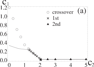
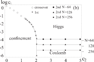
Figure 3: Phase structure in the $c_{2}$-$c_{1}$ plane of Model I with full connections $p=1$. (a) $N=64$, (b) Several $N$. As indicated, there are first-order transitions, second-order ones and crossovers. The critical value $c_{1c}$ of $c_{1}$ for $c_{2}\lesssim 2.0$ has almost no $N$ dependence, whereas $c_{1c}$ for $c_{2}\gtrsim 2.0$ behaves as $O(1/N)$. The latter $c_{1c}$ should approach to the critical value of the infinite-range Ising model $c_{1c}=1/N$ of Appendix C in the limit of $c_{2}\to\infty$ and large $N$. It gives Log(1/N)=-4.16(N=64), -4.85(N=128), -5.55(N=256), as marked on the vertical axis in (b). In (a) the dashed curves are results of MFT of Appendix D. They are almost same as MC results for $c_{2}\gtrsim 1.3$ but give first-order transitions instead of crossovers for $0\leq c_{2}\lesssim 1.3$.

Because $Z_{\rm I}$ has no singularity in $c_{1}$, there are no phase transitions at $c_{2}=0$. This is consistent with Fig.3 where we have a crossover at $c_{2}\lesssim 1.3$. In Appendix B, we study the case $p<1$ where $U$ and $C$ are shown to have a form $U(p)=p\;U(p=0),\ C(p)=p\;C(p=0)$.

(b) In the region of large $c_{2}$ (explicitly speaking, $c_{2}\gtrsim 2.0$), fluctuations of $J_{ij}$ are small and so the $c_{2}$-term of $E_{\rm I}$ becomes almost constant. We note that the (fully-connected) $c_{2}$-term of the energy has the lowest value $U=-c_{2}{}_{N}C_{3}/N$ at $J_{ij}J_{jk}J_{ki}=1$ for all the triangle $ijk$. This is achieved by the trivial configuration $J_{ij}=1$ and its gauge transformed ones[18].

To estimate the critical value $c_{1c}$ in this region, one may set $J_{ij}=1$. Then the behavior of the system at $p=1$ is controlled by the $c_{1}$-term with $J_{ij}=1$. That is, the system reduces to the so-called infinite-range Ising (IRI) spin model, the energy $E_{\rm IRI}$ of which is given by

$$E_{\rm IRI}=-c_{1}\sum_{i<j}S_{i}S_{j}.$$ (3.2)

In Appendix C we analyze the IRI model by the saddle-point method, which gives rise to the exact result for $N\to\infty$. We see there that the nontrivial phase structure is obtained for small $c_{1}$ such that $c_{1}\propto N^{-1}$. In fact, there is a second-order phase transition at $c_{1}N=1$. Then, if we consider the internal energy $U_{1,2}$ and the specific heat $C_{1,2}$ of the $c_{1,2}$-term of the energy separately as

$$E_{\rm I} = E_{1}+E_{2},$$

$$U_{a} = \langle E_{a}\rangle,\ C_{a}=\langle E_{a}^{2}\rangle-\langle E_{a}\rangle^{2},\ (a=1,2),$$ (3.3)

we expect $U_{1},C_{1}=O(N),\ U_{2},C_{2}=O(N^{2})$ for $c_{2}\gtrsim 2.0$. That is, the magnitudes of $U_{a},C_{a}$ are of different order for $a=1,2$ for the choice $c_{1}=O(N^{-1})$ and $c_{2}=O(N^{0})$. This consideration is supported by Fig.3b, which shows that the exact value of $c_{1c}$ for $c_{2}\gtrsim 2.0$ is very near to the value of IRI model, i.e., $c_{1c}=1/N$. The discrepancy is attributed to the corrections of $O(N^{-2})$ and $O(c_{2}^{-1})$.

At first, it may sound strange to have a phase transition for $c_{2}\gtrsim 2.0$ because $U_{1}$ and $U_{2}$ are unbalanced there. However, that transition is not due to the competition between these two terms, but the competition between the energy and entropy of the $c_{1}$-term itself (with fixed $J_{ij}$’s) as explained above. Therefore, that unbalance does not matter.

On the contrary, as we shall see, in the region $c_{2}\lesssim 2.0$, the critical value $c_{\rm 1c}$ of $c_{1}$ is $O(N^{0})$, which is almost independent of $N$. Then, both $U_{1}$ and $U_{2}$ is of $O(N^{2})$ with $c_{1},c_{2}=O(N^{0})$. In summary, we always take $c_{2}=O(N^{0})$, and therefore $U_{2}=O(N^{2})$, whereas we allow $c_{1}$ to vary from $O(N^{-1})$ to $O(N^{0})$, so $U_{1}$ varies from $O(N)$ to $O(N^{2})$ accordingly.

(c) Let us comment on the phase structure obtained by MFT based on a variational principle[19], which is summarized in Appendix D. As shown in Fig.3a, it predicts that the first-order confinement-Higgs transition continues down to $c_{2}=0$ instead of the MC results which has an end point $c_{2}\simeq 1.3$ at which the first-order terminates and becomes crossover. We note here that this MFT does not necessarily predict the correct results even in the limit $N\to\infty$ in contrast with the Sherrington-Kirkpatrick model[13]. This is due to the $c_{2}$-term which has mutual couplings among $J_{ij}$.

Let us see the details of each phase transition(crossover) in Fig.3. We consider the following four cases (i)-(iv) in order.

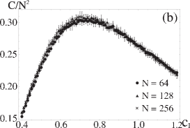
Figure 4: (a) $U/N^{2}$ and (b) $C/N^{2}$ of Model I at $c_{2}=0.5$ and $p=1.0$. There is no systematic development of the peak of $C$, so there are no transitions but a crossover.

(i) Between confinement and Higgs phases($0\leq c_{2}\lesssim 1.3$)

In Fig.4 we present $C$ and $U$ between the confinement and Higgs phases at $c_{2}=0.5$. The round peak of $C$ has no development as $N$ increases. So we conclude that there is only a crossover between these two phases. This is consistent with the above argument (a) for $c_{2}=0$ that there is no phase transition along $c_{2}=0$.

(ii) Between confinement and Higgs phases($1.3\lesssim c_{2}\lesssim 2.0$)

In Fig.5 we present $C/N^{2}$ and $U/N^{2}$ for $c_{2}=1.4$. The peak of $C$ is sharp and develops rapidly as $N$ increases, and also $U$ exhibit a jump (small hysteresis). So we conclude that there is a first-order transition between these two phases in this region of $c_{2}$.

(iii) Between Higgs and Coulomb phases($2.0\lesssim c_{2}$)

In Fig.6 we present $U_{a}$ and $C_{a}$ of Eq.(3.3) for $c_{2}=10.0$. There is a systematic $N$ dependence of the peak of $C_{1}/N$, indicating a second-order transition at $c_{1}\simeq 1/N$. This is consistent with the above result (b) of IRI spin model that corresponds to $c_{2}=\infty$. The critical value $c_{1c}N$ approaches to 1 as expected.

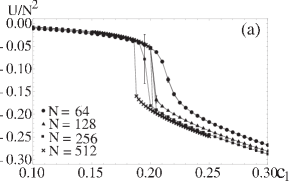
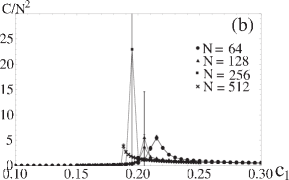
Figure 5: (a) $U/N^{2}$, (b) $C/N^{2}$ of Model I vs. $c_{1}$ at $c_{2}=1.4$ and $p=1.0$. There is a hysteresis in $U$, and the peak of $C$ develops rapidly as $N$ increases. So there is a first-order transition at $c_{1}\simeq 0.2$.

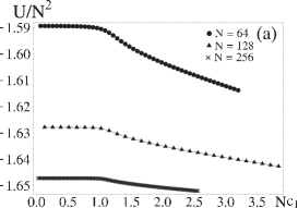
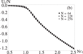
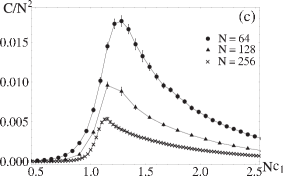
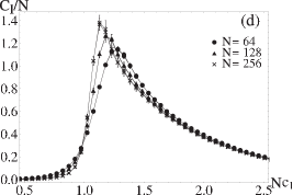
Figure 6: (a) $U/N^{2}$, (b) $U_{1}/N$, (c) $C/N^{2}$ and (d) $C_{1}/N$ of Model I vs. $Nc_{1}$ at $c_{2}=10.0$ and $p=1.0$ ($U_{1}$ and $C_{1}$ are defined in Eq.(3.3)). There is a second-order transition at $c_{1}\simeq O(1/N)$. In the limit of $c_{2}\to\infty$ and $N\to\infty$, the peak location of $C$ should approach to the value $Nc_{1c}=1.0$ of the IRI model of Appendix C.

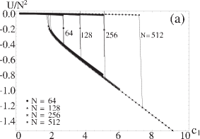
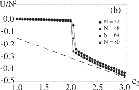
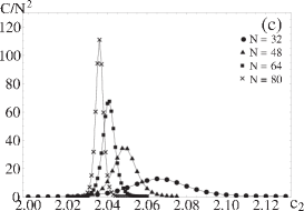
Figure 7: $U/N^{2}$ and $C/N^{2}$ of Model I at $c_{1}=0.0$ and $p=1.0$. (a) $U/N^{2}$ by Metropolis updates, (b) $U/N^{2}$ and (c) $C/N^{2}$ by multicanonical method. The hysteresis in $U$ and the strongly $N$-dependent development of the sharp peak in $C$ exhibit a first-order transition. The range of hysteresis in $U$ is reduced significantly by multicanonical method. The dashed line in (b) shows $U/N^{2}=-{}_{N}C_{3}c_{2}/N^{3}$ with $N=80$ for the completely ordered case $J_{ij}J_{jk}K_{ki}=1$.

(iv) Between confinement and Coulomb phases

In Fig.7 we present $U/N^{2}$ and $C/N^{2}$ for $c_{1}=0.0$. There is a sharp $N$ dependence of the peak of $C$ and hysteresis on $U$, so there is a first-order transition. This is in contrast to Model 0, which exhibits a second-order transition between the confinement and Coulomb phases[4]. We note that this difference of the order of the transition at $c_{1}=0$ does not come from the difference of the power of the $c_{2}$ interaction, i.e., the quartic one $JJJJ$ and the cubic one $JJJ$. In fact, the MFT of Appendix D supports this interpretation explicitly, because it predicts a first-order transition for both cases (See Ref.[4] and Appendix D). This difference of the transition order should reflect the difference of connectivity, that is $p=1.0$ in Model I and $p=O(1/N)$ in Model III (See discussion of Sect.3.2 for more details).

In the Coulomb phase, the configuration of $J_{ij}$ is strongly ordered after the transition at $c_{2}\sim 2.0$. In fact, Fig.7b shows that $U/N^{2}$ is near its saturated value $U/N^{2}=-{}_{N}C_{3}c_{2}/N^{3}$ (shown by the dashed line) which is given by setting $J_{ij}J_{jk}J_{ki}=1$.

We also note that the straightforward Metropolis algorithm (Fig.7a) gives rise to a huge hysteresis in $U$, while a multicanonical method (Fig.7b,c) gives rise to a moderate hysteresis. The latter is useful to locate a more accurate location of the transition point.

3.2 partial connections ($p<1$)

Let us consider the phase structure for partial connections. In Fig.8 we present the phase diagram in the $c_{2}$-$c_{1}$ plane for $p=0.9,0.5,0.3$ in which we plot the location of the peak of $C$. As in the case of $p=1.0$, this peak exhibits crossover for the small $c_{2}$ region ($p^{2}c_{2}\lesssim 1.3$) and first-order transitions for $1.3\lesssim p^{2}c_{2}\lesssim 2.0$. The curves for $2.0\lesssim p^{2}c_{2}$ are of second-order transitions, which have the critical value $c_{1c}\propto 1/N$ for general $N$ as explained for $p=1.0$.

In Fig.8b we present the critical curves $c_{1c}$ with various $p$ in the $p^{2}c_{2}$-$c_{1}$ plane, which show that they have almost a scaled universal curve $c_{1}=c_{1c}(p^{2}c_{2})$. This may sound strange because one may expect that the effective couplings scale as $c_{1}\epsilon_{ij}\to pc_{1}$ and $c_{2}\epsilon_{ij}\epsilon_{jk}\epsilon_{ki}\to p^{3}c_{2}$. However, it is too simple and the reason of this scaling can be suggested from the result for the case of $c_{2}=0.0$. The exact study in Appendix B gives rise to the location of the peak of $C$ at $c_{1}\simeq 1.20$, which is determined by the equation $c_{1}\tanh c_{1}=1$ [See Eq.(B.16)] and has no $p$ and $N$ dependences, because both $C$ and $U$ are proportional to $p$ there. Thus one may expect for the general case of $c_{2}\neq 0$ that $U\sim Npc_{1}u_{1}+N^{2}p^{3}c_{2}u_{2}=p[Nc_{1}u_{1}+N^{2}p^{2}c_{2}u_{2}]$ with $u_{1},u_{2}=O(N^{0}p^{0})$. Then the relevant parameters may become $c_{1}$ and $p^{2}c_{2}$, which are in fact the case as Fig.8b shows.

Let us comment on the confinement-Coulomb transition, which, for $p=1.0$, is of first-order and takes place at $c_{2}\simeq 2.0$. For $p<1.0$, it remains of first-order and takes place at $p^{2}c_{2}\simeq 2.0$. We recall that the lattice model, Model 0, gives rise to a second-order confinement-Coulomb transition. Because the connectivity of Model 0 may be estimated as $p\simeq 3N/{}_{N}C_{2}\simeq 6/N$, Model 0 may be viewed as Model I in a special limit of dilute connectivity $p\sim 0$. And therefore one may expect that the confinement-Coulomb transition of Model I becomes of second-order as $p$ becomes sufficiently small, for $p<p_{c}(\neq 0)$. It is a future problem to estimate the possible critical value $p_{c}$ (The exponent $\alpha$ of $p_{c}=O(N^{\alpha})$ may be 0 or -1, or other nontirivial value).

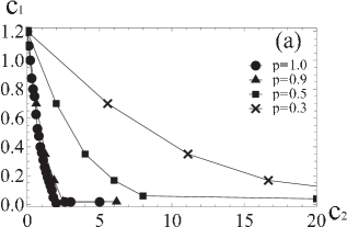
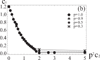
Figure 8: Phase diagram of Model I with partial connectivities, $p=0.9,0.5,0.3$ together with $p=1$ ($N=64$) (a) in the $c_{2}$-$c_{1}$ plane and (b) in the $p^{2}c_{2}$-$c_{1}$ plane. In (b), the curves for $0<p^{2}c_{2}\lesssim 1.3$ show crossover, $1.3\lesssim p^{2}c_{2}\lesssim 2.0$ show first-order transitions, and those for $2.0\lesssim p^{2}c_{2}$ show second-order transitions. The critical values in the region of $2.0\lesssim p^{2}c_{2}$ is $c_{1c}=O(N^{-1})$ for general $N$.

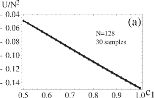
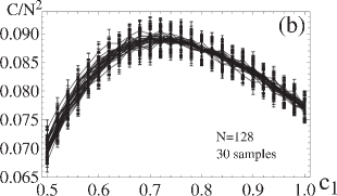
Figure 9: (a) $U/N^{2}$ and (b) $C/N^{2}$ of Model I at $p=0.3,c_{2}=5.555$ for 30 samples. Each curve is for each sample and the error bars are errors in thermal(MC) averages. The deviations over samples are smaller than MC errors.

We note that Fig.8 is obtained by using a set of data $U$ and $C$ of only one sample, because we have checked that the location of $C$ has small deviation over different samples. For example, in Fig.9 we present $U$ and $C$ along $c_{2}=5.555(p^{2}c_{2}=0.5)$ for 30 samples with p=0.3. There are 30 curves with each curve for each sample. The error bars in Fig.9 denote errors associated with MC sweeps (thermal average) of each sample. Fig.9 shows that the deviations of $U,C$ over samples are smaller than these errors by factor $\sim 2$. So we judge that the result of one sample is reliable for $0.3\leq p\leq 1.0$.

4 Model II: Quenched model with full connections

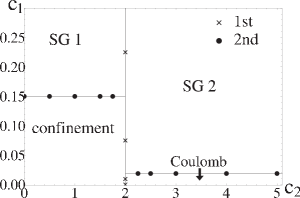
Figure 10: Phase diagram of Model II in the $c_{2}$-$c_{1}$ plane for $N=64$. There are four phases separated by boundaries with 1st and 2nd-order transitions as indicated. The Higgs phase of Model I is separated to two SG phases (SG1 and SG2). The crossovers of Model I disappear and the 1st-order transitions continue down to $c_{2}=0$. The critical value of second-order transitions behaves as $c_{1c}=O(1/\sqrt{N})$ for $c_{2}\lesssim 2.0$ and $c_{1c}=O(1/N)$ for $c_{2}\gtrsim 2.0$.

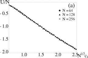
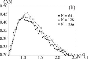
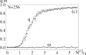
Figure 11: (a) $U/N$, (b)$C/N$ and (c) $q,m$ of Model II vs. $\sqrt{N}c_{1}$ for $c_{2}=1.5$. It shows a second-order transition into a SG1 phase. $m$ vanishes as expected.

In this section we study the phase structure of Model II. In Fig.10 we first present its phase diagram in the $c_{2}$-$c_{1}$ plane. Here we recall that the configurations of synaptic variables $J_{ij}$ are completely determined by $P(J)$ of (2.15). From the analysis of Sect.2.1 for $c_{1}=0.0$, $P(J)$ describes a first-order phase transition at $c_{2}\simeq 2.0$ for $p=1.0$. This transition at $c_{2}\simeq 2.0$ survives in Model II for all $c_{1}$.

Fig.10 shows that there are other two phase transition lines, both of which is of second order. One is in the region $c_{2}\lesssim 2.0$ at $c_{1c}\simeq 0.15$ for $N=64$ and separates the confinement phase $c_{1}<c_{1c}$ and the another phase $c_{1}>c_{1c}$. We call this phase $c_{1}>c_{1c}$ a SG phase (we call it SG1 phase) as we shall see that the SG order parameter $q$ is nonvanishing there. Also we shall see that the value of $c_{1c}$ scales as $c_{1c}\propto 1/\sqrt{N}$ as $N$ increases.

The other transition line is in the region $c_{2}\gtrsim 2.0$ at $c_{1c}\simeq 0.02$ for $N=64$ and separates the Coulomb phase $c_{1}<c_{1c}$ and another SG phase for $c_{1}>c_{1c}$ (we call it SG2 phase). The value of $c_{1c}$ scales as $c_{1c}\propto 1/N$ as $N$ increases, which is similar to Model I.

Let us see each transition in details.

(i) confinement-SG1 transition

In Fig.11 we present $U$, $C$, $m$ and $q$ vs. $\sqrt{N}c_{1}$ for $c_{2}=1.5$. The $N$ dependence of the peak of $C$ indicates a second-order transition. The behavior of $m$ and $q$ show that the phase of higher $c_{1}$ is the SG phase.

In Model I, the exact treatment for $c_{2}=0$ in Appendix B exhibits a crossover as $c_{1}$ varies. The reason that Model II exhibits a second-order transition line in this region ($0\leq c_{2}\leq c_{2c}$) instead is traced back to our treatment of $J_{ij}$ as quenched variables. In Appendix E we make use of the resemblance of Model II at $c_{2}=0$ and the Sherrington-Kirkpatrick model [13] of SG, and present a plausible argument that Model II for $c_{2}=0$ has a second-order transition at $c_{1}\propto 1/\sqrt{N}$.

This result $c_{1c}\propto 1/\sqrt{N}$ for $c_{2}\lesssim 2.0$ can be also understood as a compromise of the two results; (a) $c_{1c}=O(N^{-1})$ of annealed Model I for $c_{2}\gtrsim 2.0$ where $J_{ij}$ are almost ordered, and (b) $c_{1c}=O(N^{0})$ of Model I for $c_{2}\lesssim 2.0$ where $J_{ij}$ are random. In fact, configuration of $J_{ij}$ in each sample of the quenched Model II for $c_{2}\lesssim 2.0$ is almost fixed, but the spatial average of $J_{ij}J_{jk}J_{ki}$ is much less than its saturated value 1. Therefore the effect of $J_{ij}$ may be smaller than the complete order in the case (a) but larger than the complete randomness in the case (b).

(ii) Coulomb-SG2 transition

In Fig.12 we present $U/N$, $C/N$ and $q$ vs. $Nc_{1}$ for $c_{2}=2.5$. The $N$ dependence of the peak of $C$ indicates a second-order transition at $Nc_{1}\simeq 1.15$. The behavior of $q$ shows that the phase of higher $c_{1}$ is the SG phase.

Fig.12d shows $C/N$ of 200 samples (different configurations of $J_{ij}$); each curve is for each sample. It shows that the deviations over samples are smaller than typical errors in thermal average over different $S_{i}$. Therefore we judge that 200 samples are sufficient to obtain the location of specific heat along a fixed $c_{2}$ semiquantitatively.

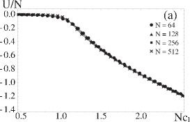
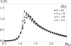
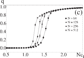
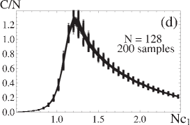
Figure 12: (a)$U/N$, (b)$C/N$, (c)$q$, (d) $C/N$ of Model II vs. $Nc_{1}$ for $c_{2}=2.5$. They exhibit a second-order transition at $Nc_{1}\simeq 1.15$. (d) shows 200 curves of $C/N$ for 200 samples of quenched variables $J_{ij}$ separately. Error bars in (d) are errors in MC sweeps (thermal average), which are larger than the deviations over samples.

(iii) Transition across the $c_{2}\simeq 2.0$ line

As explained, this first-order transition curve reflects $P(J)$ of (2.15) as already shown in Fig.7 for Model I at $c_{1}=0$. Explicit calculation of $U$ and $C$ across this transition for fixed $c_{1}$ is time-consuming because one needs multicanonical method due to large hysteresis of Metropolis updates as Fig.7a shows. In place of such a calculation, in Fig.13 we present $U/N^{2}$, $C/N^{2}$ of (2.17) and $q$, which are calculated with Metropolis updates by selecting runs along the lower-energy branch of the hysteresis curve in Fig.7a. These runs are realized by a cold start such as $S_{i}=J_{ij}=1$ and the results are reliable qualitatively because the transition point $c_{2c}\simeq 1.85(N=64)$ determined by this method is not far from the true value $c_{2c}\simeq 2.04$ given in Fig.7b,c ($\sim 10\%$ deviation). In Fig.13g,h we also present $U_{2}$ and $C_{2}$ for the $c_{2}$-term defined by

$$E_{2} \equiv -\frac{c_{2}}{N}\sum_{i<j<k}J_{ij}J_{jk}J_{ki},$$

$$U_{2} \equiv -\langle E_{2}\rangle,\ C_{2}\equiv\langle E_{2}^{2}\rangle-\langle E_{2}\rangle^{2},$$ (4.1)

and calculated by this Metropolis updates. These definitions are equivalent to $U,C$ of Model I at $c_{1}=0$, and therefore they should be compared with Fig.7b,c. Actually they have no significant differences.

Fig.13f shows that $q$ has a jump $\Delta q\simeq 0.4$ across the SG1-SG2 phase transition, and $q\simeq 1$ in SG2 phase. It shows the difference of two SG phases clearly.

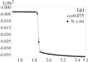
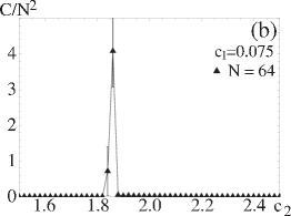
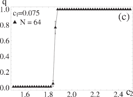
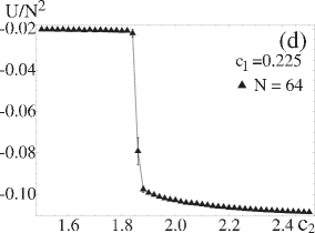
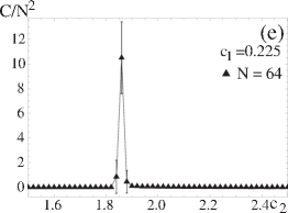
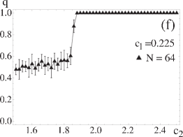
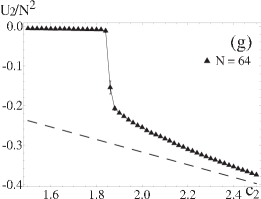
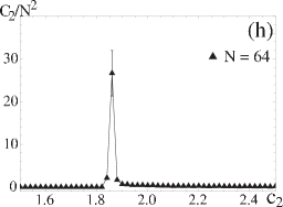
Figure 13: Metropolis calculations of $U/N^{2}$, $C/N^{2}$ and $q$ of Model II at (a-c) $c_{1}=0.075$ for the confinement-SG2 transition and at (d-f) $c_{1}=0.225$ for the SG1-SG2 transition. Both of them are of first-order. (g) $U_{2}/N^{2}$ and (h) $C_{2}/N^{2}$ are defined in Eq.(4.1) and should be compared with Fig.7b,c of multicanonical calculations. The dashed line in (g) is $U_{2}/N^{2}=-c_{2}{}_{N}C_{3}/N$ for $N=64$ corresponding to the saturated value $J_{ij}J_{jk}J_{ki}=1$.

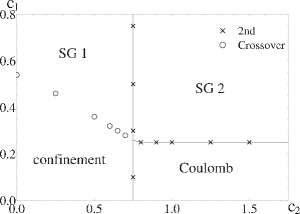
Figure 14: Phase structure of Model III, the quenched 3D lattice model, in the $c_{2}$-$c_{1}$ plane. The boundaries are determined by the location of the specific heat $C$ for $N=12^{3}$. The second-order confinement-SG1 transition in Model II becomes crossover.

5 Model III: Quenched lattice model

In this section we study the phase structure of Model III. In Fig.14 we present the phase diagram in the $c_{2}$-$c_{1}$ plane. The overall phase structure is similar to that of Model II, but the second-order transition between the confinement and the SG1 phases of Model II ($c_{2}\lesssim 2.0$) becomes a crossover. This may be accounted for by the fact that the connectivity among $S_{i}$ in Model III is restricted to the nearest-neighbor neurons and much weaker than in Model II. The argument of obtaining the second-order transition for Model II by referring to the Sherrington-Kirkpatrick model in Appendix E fails due to the scarce connectivity of Model III, which does not validate the saddle-point estimation of Ref.[13]. Therefore, it is harder to obtain an ordered phase of $S_{i}$ in Model III compared with Model II.

Furthermore, the critical value $c_{1c}$ for $c_{2}\gtrsim 2.0$ depends on $N$ weakly, but it is almost constant in contrast with $1/N$-dependence of Model I and Model II. This is also due to the scarce connectivity and consistent with the previous result for annealed 3D model in which $c_{1c}$ for $c_{2}\gtrsim 2.0$ is $O(N^{0})$ (Note there is no extra factor $N^{-1}$ in the $c_{2}$-term in Eq.(2.1) and Eq.(2.23)).

Let us see each phase transition and crossover.

(i) Crossover between the confinement and SG1 phases

In Fig.15 we present $U/N$, $C/N$ and $q$ vs. $c_{1}$ for $c_{2}=0.5$. $C/N$ shows a crossover between confinement and SG1 phases because it has almost no $N$ dependence.

(ii) Coulomb-SG2 transition

In Fig.16 we present $U/N$, $C/N$ and $q$ vs. $c_{1}$ for $c_{2}=1.0$. $C/N$ shows a second-order transition between Coulomb and SG2 phases because its peak develops systematically as $N$ increases.

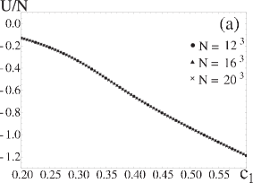
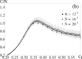
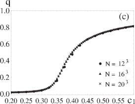
Figure 15: (a) $U/N$, (b) $C/N$, (c) $q$ of Model III vs. $c_{1}$ for $c_{2}=0.5$. There are no sharp transitions but a crossover between the confinement and SG1 phases at $\sqrt{N}c_{1}\simeq 0.35\sim 0.40$.

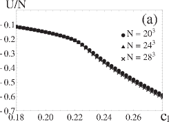
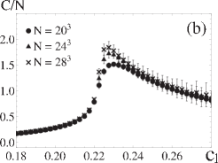
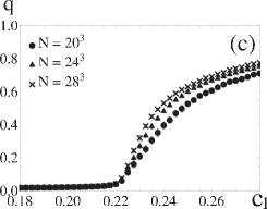
Figure 16: (a) $U/N$, (b) $C/N$, and (c) $q$ of Model III vs. $c_{1}$ for $c_{2}=1.0$. There is a second-order transition between the Coulomb and SG2 phases at $c_{1}\simeq 0.225$.

(iii) Transition across the line $c_{2}\simeq 0.75$.

Because the system is quenched one, this second-order transition reflects the $c_{2}$-term of the energy. It has been studied in Model 0 at $c_{1}=0$[4]. In this case, after the duality transformation, this pure-gauge system becomes equivalent to the Ising spin model in three-dimensions, which is well known to exhibit a second-order transition. In Fig.17 we present $U$ and $C$ at $c_{1}$=0.1 and 1.0. They exhibit a second-order transition as expected.

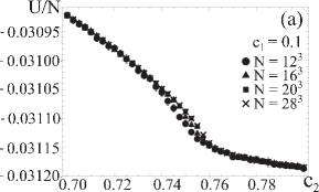
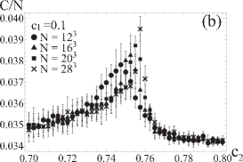
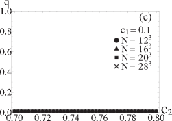
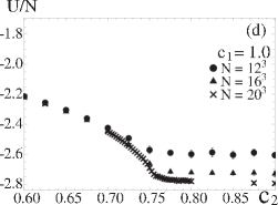
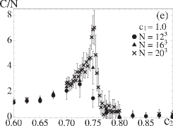
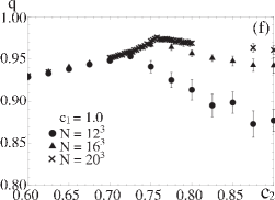
Figure 17: $U/N,C/N$ and $q$ of Model III at (a-c) $c_{1}=0.1$ and (d-f) $c_{1}=1.0$. They show a second-order transition reflecting $P(J)$ of (2.23).

6 Conclusions and Discussions

In this paper we have studied three versions of the Z(2) gauge neural network, Models I, II, and III, and compared them each other and with the annealed 3D lattice model (Model 0). The effect of reverberating signals is, in short, to enhance the order and stability of synaptic connections $J_{ij}$. For example, as $c_{2}$ is increased along the line of $c_{1}=0$, the confinement phase for $c_{2}<c_{2c}$ is converted to the Coulomb phase for $c_{2}>c_{2c}$ (See Figs.3, 10, 14).

Concerning to the phase structure, the obtained phases and the order of transitions are summerized in Table 3. These results are consistent each other; one may interpret them in a coherent manner considering how each term of $U$ and $C$, critical values $c_{1c}$ and $c_{2c}$, and the order of transition depend on the total number of sites $N$ and their connectivity $p$ as discussed in Sect.3-5.

Model	Higgs-confinement	confinement-Coulomb	Coulomb-Higgs
0	CO-1st	2nd	2nd
I	CO-1st	1st	2nd

Model	Across $c_{2}=c_{2c}$ line	SG1-confinement	SG2-Coulomb
II	1st($c_{2c}\simeq 2.0$)	2nd	2nd
III	2nd($c_{2c}\simeq 0.75$)	CO	2nd

Table3. Orders of phase transitions for various models. CO implies crossover. The upper table is for the annealed models, Models 0 and I, and the lower table is for the quenched models, Models II and III, where SG1 is the phase at $c_{2}<c_{2c}$ and SG2 is at $c_{2}>c_{2c}$.

For the annealed model, Model I, the obtained phases are same as three phases of Model 0, but the order of confinement-Coulomb transition becomes 1st order instead of 2nd order. As discussed in Sec.3.1, this reflects the difference of connectivity.

For the quenched models, Models II and III, the Higgs phase of the annealed models is better classified as the SG phase. Actually, the quenched transition at the critical value $c_{2}=c_{2c}$, which is independent of $c_{1}$, partitions the Higgs phase into two separate SG phases, SG1 ($c_{2}<c_{2c}$) and SG2 ($c_{2}>c_{2c}$). These two phases are both characterized by nonvanishing SG order parameter $q$, but are distinguished by disorder (SG1) and order (SG2) of gauge variables $J_{ij}$ as explained by using Fig.13f,g. This is another example of the effect of reverberating signals.

There we introduced $U_{2}=\langle E_{2}\rangle$ and $C_{2}$ defined in (4.1). We note that this $U_{2}$ may be viewed as an example of Wilson loop. In the usual lattice gauge theory without matter fields, which has only a plaquette interaction $JJJJ$, the confinement phase and the Coulomb phase are distinguished by the behavior of the Wilson loop[8] as

$$W[C] \equiv \langle\prod_{C}J_{x\mu}\rangle\sim\left\{\begin{array}[]{ll}\exp(-\alpha S)&{\rm confinement\ phase}\\ \exp(-\alpha^{\prime}P)&{\rm Coulomb\ phase},\\ \end{array}\right.$$ (6.2)

where the product is taken along a closed loop $C$ on the lattice, and $S$ is the minimum area having its edge $C$, and $P$ is the perimeter of $C$.

To examine the critical properties of the present models, it is necessary to study their scaling properties such as critical exponents of their second-order transitions by applying finite-size scaling argument to MC results, although such a study is beyond the scope of the present paper. Concerning to this point, we recall a work by Hashizume and Suzuki[20]. They studied the 3D lattice model, which is equivalent to the present model[21], Model 0 and Model III at $c_{1}=0$, by a kind of MFT and correlation identities, and obtained approximately the transition temperature, scaling functions, and critical exponents, etc. Such an analytical and simple method may give us some hints to calculate approximate critical exponents and related quantities for other cases of the models studied in the present paper.

As general subjects for future investigations of the Z(2) gauge neural network, following points may be listed up as interesting extension of the models themselves.

- In this paper, we restricted ourselves to the region of $c_{1},c_{2}\geq 0$. We chose this region because the $c_{1}$-term with $c_{1}>0$ may be regarded as a rescaled energy of the Hopfield model and the $c_{2}$-term of reverberating signals corresponds to the energy of magnetic field for $c_{2}>0$[8]. Study beyond this region may lead us to some new phases and transitions among them[22].

- We put the constraint $|J_{ij}|=1$ for the synaptic strength for simplicity. Even if one uses other distribution of $J_{ij}$ with same mean and covariance in place of $|J_{ij}|=1$, the global phase structure should be unchanged as long as one uses the same energy as argued in Ref.[23]. However, modification of the energy together with relaxing $J_{ij}$ to $0\leq|J_{ij}|<\infty$ will serve as a model to investigate spontaneous distribution of $|J_{ij}|$[24]. This is an interesting possibility because some parts of the human brain has a log-normal distribution of $|J_{ij}|$ which is a key structure to explain some activities of the human brain[25].

- One may consider nontirivial structure of connectivity $\epsilon_{ij}$ such as a small-world network[26], etc. This is interesting because the actual network structure of some parts of the human brain are known to be small-world type.

- It is of interest to study the asymmetric case with two independent gauge variables, $J_{ij}$ and $J_{ji}$ for a pair $i<j$[11]. This case is expected to describe some interesting effects such as spontaneous oscillations in time-development of the system.

Appendix A Elitzur’s theorem for quenched systems

In this appendix we derive Elitzur’s theorem for quenched systems. Let us start by a brief derivation of the theorem for the annealed model, Model I. The average $\langle O(S,J)\rangle$ of (2.10) is written in the form,

$$\langle O(S,J)\rangle = \sum_{S}\sum_{J}O(S,J)\exp(-E(S,J)).$$ (A.4)

Here it is sufficient to consider the average over each sample with definite $\epsilon_{ij}$, because the final average is just the sum (2.12) of such average. By regarding the gauge transformation (2.9) as a change of variables $S_{i}\to S^{\prime}_{i},\ J_{ij}\to J^{\prime}_{ij}$, $O(S,J)$ of (A.4) is rewritten as

$$\langle O(S,J)\rangle = \sum_{S^{\prime}}\sum_{J^{\prime}}O(S^{\prime},J^{\prime})\exp(A(S^{\prime},J^{\prime}))$$ (A.5)

$$= \sum_{S}\sum_{J}O(S^{\prime},J^{\prime})\exp(A(S,J))=\langle O(S^{\prime},J^{\prime})\rangle,$$

where we used

$$A(S^{\prime},J^{\prime})=A(S,J),\quad\sum_{S^{\prime}_{i}}=\sum_{S_{i}},\quad\sum_{J^{\prime}_{ij}}=\sum_{J_{ij}}.$$ (A.6)

Let us restrict $O(S,J)$ to those satisfying

$$O(S^{\prime},J^{\prime})=G(V)O(S,J).$$ (A.7)

Then (A.5) claims that

$$\langle O(S,J)\rangle=G(V)\langle O(S,J)\rangle.$$ (A.8)

If $O(S,J)$ is a gauge-invariant quantity, then $G(V)=1$, and (A.8) poses no restrictions to $\langle O(S,J)\rangle$. If $O(S,J)$ is a gauge-variant quantity, then $G(V)\neq 1$ and the following theorem is derived,

$${\rm If\ }O(S,J)\ {\rm is\ gauge\ variant,\ then}\ \langle O(S,J)\rangle=0.$$ (A.9)

For a general $O(S,J)$ that does not satisfy (A.7), it may be expressed as a sum

$$O(S,J) = \sum_{\ell}O_{\ell}(S,J),$$

$$O_{\ell}(S^{\prime},J^{\prime}) = G_{\ell}(V)O_{\ell}(S,J).$$ (A.10)

Then it is straightforward to derive the theorem (A.9).

Let us consider the quenched model, Model II for example. The average is given by (2.15),

$$\langle O(S,J)\rangle = \sum_{J}\sum_{S}O(S,J)\frac{\exp(-E_{1}(S,J))}{Z_{1}(J)}P(J),$$

$$Z_{1}(J) = \sum_{S}\exp\left(-E_{1}(S,J)\right).$$ (A.11)

We repeat the same change of variables (2.9) and note the gauge invariance,

$$E_{1}(S^{\prime},J^{\prime})=E_{1}(S,J),\ Z_{1}(J^{\prime})=Z_{1}(J),\ P(J^{\prime})=P(J),$$ (A.12)

to get

$$\langle O(S,J)\rangle=\langle O(S^{\prime},J^{\prime})\rangle.$$ (A.13)

Then we follow the same steps as for the annealed model to arrive at the theorem (A.9).

Appendix B Exact solution for $c_{2}=0$

In this Appendix, we study the exact solution of Model I for $c_{2}=0$. The partition function for a sample with a definite $\epsilon_{ij}$ is calculated as

$$Z_{c_{2}=0}(\epsilon) = \sum_{S}\sum_{J}\exp(-E_{c_{2}=0}(\epsilon))=\sum_{S}\sum_{J}\exp(c_{1}\sum_{i<j}\epsilon_{ij}J_{ij}S_{i}S_{j})$$ (B.14)

$$= \sum_{S}\prod_{i<j}\sum_{J_{ij}=\pm 1}\exp(c_{1}\epsilon_{ij}J_{ij}S_{i}S_{j})$$

$$= \sum_{S}\prod_{i<j}\left[\exp(c_{1}\epsilon_{ij}S_{i}S_{j})+\exp(-c_{1}\epsilon_{ij}S_{i}S_{j})\right]$$

$$= \sum_{S}\prod_{i<j}\left[2\delta_{\epsilon_{ij},1}\cosh c_{1}+2\delta_{\epsilon_{ij},0}\right]$$

$$= 2^{N}\prod_{i<j}\left[2\delta_{\epsilon_{ij},1}\cosh c_{1}+2\delta_{\epsilon_{ij},0}\right].$$

Then the partition function $Z_{c_{2}=0}$ averaged over samples is given by

$$Z_{c_{2}=0} = \frac{1}{N_{\epsilon}}\sum_{\epsilon}\delta_{p(\epsilon),p}Z_{c_{2}=0}(\epsilon)=2^{N}\left(2\cosh c_{1}\right)^{\frac{N(N-1)}{2}p}2^{\frac{N(N-1)}{2}(1-p)},$$ (B.15)

where we used the fact that the number of links of $\epsilon_{ij}=1(0)$ in a sample is ${}_{N}C_{2}p\ [{}_{N}C_{2}(1-p)]$. Then the internal energy $U$ and the specific heat $C$ are calculated as

$$U = \langle E\rangle_{p}=-c_{1}\frac{d}{dc_{1}}\ln Z_{c_{2}=0}=-\frac{N(N-1)}{2}pc_{1}\tanh c_{1},$$

$$C = \frac{dU}{dT}=-c_{1}^{2}\frac{d}{dc_{1}}\left(\frac{U}{c_{1}}\right)=\frac{N(N-1)}{2}\frac{p\;c_{1}^{2}}{\cosh^{2}c_{1}}.$$ (B.16)

We note that $U$ and $C$ are proportional to $p$ as it should be. We have checked that the MC results agree with these results as shown in Fig.18.

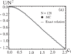
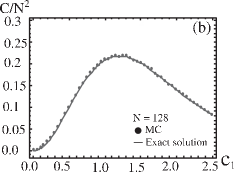
Figure 18: The MC results of (a) $U$ and $(b)C$ of Model I at $c_{2}=0$ for $p=1.0$ and $N=128$. They agree with the analytic expressions of (B.16).

Appendix C Infinite-Range Ising spin model

Let us study the IRI spin model (3.2). The partition function is rewritten as

$$Z_{\rm IRI} = \sum_{S}\exp(c_{1}\sum_{i<j}S_{i}S_{j})=\sum_{S}\exp(\frac{c_{1}}{2}\sum_{i,j}S_{i}S_{j}-\frac{c_{1}}{2}N)$$

$$= \exp(-\frac{c_{1}}{2}N)(2\pi c_{1})^{-\frac{1}{2}}\sum_{S}\int_{-\infty}^{\infty}d\chi\exp(-\frac{1}{2c_{1}}\chi^{2}+\chi\sum_{i}S_{i})$$

$$= \exp(-\frac{c_{1}}{2}N)(2\pi c_{1})^{-\frac{1}{2}}\int_{-\infty}^{\infty}d\chi\exp\left(-\frac{1}{2c_{1}}\chi^{2}+N\ln(2\cosh\chi)\right)$$

$$= \exp(-NF_{\rm IR}+O(N^{0})),$$

$$F_{\rm IRI} = \frac{1}{2c_{1}N}\chi_{0}^{2}-\ln(2\cosh\chi_{0}),$$ (C.17)

where we assumed that $c_{1}=O(N^{-1})$ and used the saddle-point evaluation for large $N$. $\chi_{0}$ is the solution of the saddle-point equation,

$$-\frac{\chi}{Nc_{1}}+\tanh\chi=0.$$ (C.18)

$\chi_{0}$ exhibits a second-order transition at $c_{1c}=1/N$,

$$\chi_{0}\left\{\begin{array}[]{ll}=0,&Nc_{1}<1,\\ \neq 0,&Nc_{1}>1.\end{array}\right.$$ (C.21)

Appendix D Mean field theory for Model I with $p=1.0$

In this Appendix we study MFT of Model I with $p=1.0$ based on the Feynman’s method[19]. It is formulated as a variational principle for the Helmholtz free energy $F$ by using the variational (trial) energy $E_{0}$ as follows;

$$Z = \sum_{S,J}\exp(-\beta E)\equiv\exp(-\beta F),$$

$$Z_{0} = \sum_{S,J}\exp(-\beta E_{0})\equiv\exp(-\beta F_{0}),$$

$$\langle O\rangle_{0} \equiv Z_{0}^{-1}\sum_{S,J}O\exp(-\beta E_{0}),$$

$$F \leq F_{v}\equiv F_{0}+\langle E-E_{0}\rangle_{0}.$$ (D.22)

We adjust the variational parameters contained in $E_{0}$ optimally so that $F_{v}$ is minimized.

For $E_{0}$ we use

$$E_{0}=-W\sum_{i<j}J_{ij}-h\sum_{i}S_{i},$$ (D.23)

where $W$ and $h$ are real variational parameters. Then we have

$$f_{v} \equiv \frac{F_{v}}{N}=-\frac{N_{l}}{N}\ln(2\cosh\beta W)-\ln(2\cosh\beta h)$$

$$-c_{1}\frac{N_{l}}{N}m^{2}M-c_{2}\frac{{}_{N}C_{3}}{N}M^{3}+\frac{N_{l}}{N}WM+hm,$$

$$m \equiv \langle S_{i}\rangle_{0}=\tanh h,\ M\equiv\langle J_{ij}\rangle_{0}=\tanh W.$$ (D.24)

The minimization of $f_{v}$ yields the three phases characterized as follows;

(D.29)

The phase boundaries are shown in Fig.19. The discontinuity of order parameters of each transitions are as follows;

(D.34)

For the Higgs-Coulomb transition, the critical value of $c_{1}$ is estimated as

$$c_{1c}=\frac{N}{2N_{l}}\frac{1}{M}\simeq\frac{1}{N},$$ (D.35)

for large $N$ and large $c_{2}$ at which $M\simeq 1$.

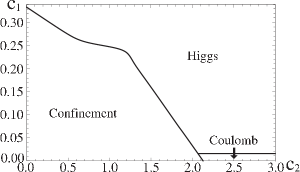
Figure 19: MFT result for the phase structure of Model I with $p=1.0$ in the $c_{2}$-$c_{1}$ plane ($N=64$). There is a first-order transition curve starting at $c_{1c}\simeq 0.334(c_{2}=0)$ and ending at $c_{1c}=0(c_{2}\simeq 2.13)$, and a second-order one along $c_{1c}\simeq 1/N(c_{2}\gtrsim 2.0)$ .

Appendix E Comparison of Model II at $c_{2}=0$ and the Sherrington-Kirkpatrick model

In this Appendix we study a possible phase transition of Model II at $c_{2}=0$ by using the known result of Sherrington-Kirkpatrick (SK) model[13].

The energy of the SK model is given by

$$E_{\rm SK} = -\sum_{i<j}J_{ij}S_{i}S_{j},\ S_{i}=\pm 1,\ J_{ij}\in(-\infty,\infty).$$ (E.36)

The quenched variable $J_{ij}$ is a real number(we use the same symbol with our $J_{ij}=\pm 1$), and distributes by the Gaussian weight,

$$P_{\rm SK}(J) = \prod_{i<j}\frac{N^{1/4}}{\sqrt{2\pi}\tilde{J}}\exp\left(-\frac{(J_{ij}-\tilde{J}_{0}/N)^{2}}{2\tilde{J}^{2}/N}\right).$$ (E.37)

Then the replica-symmetric solution for large $N$ (which is accepted as correct ones for small $J_{0}$) gives rise to a phase-diagram in the $\tilde{J_{0}}/\tilde{J}-(1/\tilde{J})$ plane in which there is a horizontal second-order phase transition line along $1/\tilde{J}=1$ for $\tilde{J_{0}}/\tilde{J}\leq 1$ separating the SG phase $m=0,q\neq 0$ ($1/\tilde{J}<1$) and the paramagnetic phase $m=0,q=0$ (1/$\tilde{J}>1$). From the point $1/\tilde{J}=1,\tilde{J_{0}}/\tilde{J}=1$, two transition curves spring out to border the ferromagnetic phase $m\neq 0,q\simeq m^{2}$ in the larger $\tilde{J_{0}}/\tilde{J}$ region (Note that Z(2) gauge symmetry is violated for $\tilde{J}_{0}\neq 0$).

Let us turn to Model II at $c_{2}=0$ and deform it by replacing $J_{ij}=\pm 1$ to a real variable with an optimally determined distribution of the form of $P_{\rm SK}$ of (E.37). We choose $P_{\rm SK}$ to generate the same mean value and variance as $P(J)$ of (2.15), i.e., $\langle J_{ij}\rangle_{P_{\rm SK}}=0,\langle J_{ij}^{2}\rangle_{P_{\rm SK}}=1$. This treatment of Z(2) variable by real Gaussian variable may preserve universal critical properties of the system[23]. This determines the optimal $P_{\rm SK}$ as

$$P_{\rm SK}(J) = \prod_{i<j}\frac{N^{1/4}}{\sqrt{2\pi}\tilde{J}}\exp\left(-\frac{J_{ij}^{2}}{2}\right).$$ (E.38)

To adjust $E_{\rm SK}$ to $E_{1}$ of (2.15), we replace $J_{ij}$ of the SK model by $c_{1}J_{ij}$. Then $P_{\rm SK}(J)$ of (E.37) becomes the same as Eq.(E.38) by choosing $\tilde{J}_{0}=0$ and

$$\frac{c_{1}^{2}}{\tilde{J}^{2}/N}=1.$$ (E.39)

Then, the established transition point of SK model for $\tilde{J}_{0}=0$, $\tilde{J}=1$ predicts the location of second-order transition of Model II at $c_{2}=0$ as

$$c_{1c}=\frac{1}{\sqrt{N}}.$$ (E.40)

This gives an estimate $c_{1c}=0.125$ for $N=64$, which should be compared with the MC result of Fig.10, $c_{1c}\simeq 0.15$. Inclusion of the $c_{2}$-term makes summation over $J_{ij}$ variables difficult analytically.

References

- [1] J. J. Hopfield, Proc. Nat. Acd. Sci. USA. 79, (1982) 2554.
- [2] See, e.g., S. Haykin,“Neural Networks; A Comprehensive Foundation”, Macmillan Pub. Co. (1994).
- [3] T. Matsui, pp. 271 in Fluctuating Paths and Fields, ed. by W. Janke et al., World Scientific (2001) (cond-mat/0112463).
- [4] M. Kemuriyama, T. Matsui and K. Sakakibara, Physica A 356 (2005) 525.
- [5] In Ref.[4], we have included the -term with . In this paper we cite the result for for simplicity. It may also help to enhance the contrast with the case with full connections of Model I.
- [6] D. O. Hebb, “The Organization of Behavior: A Neuropsychological Theory”, New York: Wiley. (1949)
- [7] We note that the -term is relevant and generated after renormalization of the -term as one can see the relation, because for Models 0 and III, and for Models I and II.
- [8] K. G. Wilson, Phys. Rev. D10 (1974) 2445; J. B. Kogut, Rev. Mod. Phys. 51 (1979) 659.
- [9] We note that, instead of a second-order one, the MFT incorrectly predicts a first-order transition for the confinement-Coulomb transition, because the number of dimensions (three) is not high enough for MFT[4].
- [10] Order parameters used in MFT conflict with Elitzur’s theorem[15], because it implies . To save the MFT results and make them compatible with Elitzur’s theorem, Drouffe [J. M. Drouffe, Nucl. Phys. B 170 (1980) 211] proposed just to average over the gauge-transformed copies of a MF solution. The thermodynamic quantities, hence the location and the nature of phase transitions, are unchanged by this averaging.
- [11] We note that, even for the general case of two independent variables and , the Hopfield energy itself is independent of the asymmetric part . On the other hands, the term reflects this asymmetry.
- [12] S. F. Edward and P. W. Anderson, J. Phys. F5 (1975) 965; M. Mezard, G. Parisi and M. A. Virasoro,“Spin Glass Theory and Beyond”, World Scientific, Singapore (1987).
- [13] D. Sherrington and S. Kirkpatrick, Phys. Rev. Lett. 35 (1979) 1792.
- [14] For the case of , one may make use of Z(2) gauge symmetry as Thoulouse [G. Toulouse, Commun. Phys. 2 (1977) 115.] adopted it to characterize effects of frustrations in SG. See also J. Vannimenus, G. Toulouse, J. Phys. C 10 (1977) L537; L. G. Marland, D. D. Betts, Phys. Rev. Lett. 43 (1979) 1618; H. Nishimori, P. Sollich, J. Phys. Soc. Jpn. 69 (2000) A160; A. Keren, J. S. Gardner, Phys. Rev. Lett. 87 (2001) 177201.
- [15] S. Elitzur, Phys. Rev. D12 (1975) 3978.
- [16] N. Metropolis, A. W. Rosenbluth, M. N. Rosenbluth, A. M. Teller, E. Teller, J. Chem. Phys. 21 (1953) 1087.
- [17] B. A. Berg and T. Neuhaus, Phys. Lett. B 267 (1991) 249; Phys. Rev. Lett. 68 (1992) 9.
- [18] Because implies all the “magnetic field” are specified, one expects that the corrsponding gauge field is unique except for its gauge transformed ones. That is, there are no degenerate configurations of that are not connected to by a gauge transformation. This can be confirmed explicitly for small number such as .
- [19] R. P. Feynman, ”Statistical Mechanics, A set of Lectures”, Chap.8, W. A. Benjamin (1972).
- [20] Y. Hashizume and M. Suzuki, Int. J. Mod. Phys. B25 (2011) 73.
- [21] As cited in Ref.[4] (as Ref.[29]), Wegner [F. Wegner, J. Math. Phys.12 (1971) 2259] performed duality transformations to relate various Ising “spin” models on -dimensional lattice. In particular, the 3D ordinary Ising spin model is equivalent to the present Model 0(III) at [See Sec.5, point (iii)]. The former is well known to exhibit a second-order phase transition at the corresponding point . The gauge variable on the link is called there as a generalized “spin”, so that the gauge model is a “spin” model with a four-spin interaction. Suzuki [M. Suzuki, Phys. Rev. Let. 28 (1972) 507] considered a related 3D model, i.e., a model with four-spin interaction only in the - and -planes, and obtained an exact solution. The system is duality-equivalent to a collection of decoupled 2D Ising models, each of which is defined for every 12-plane. This system also exhibits a second-order transition but has no spontaneous magnetization.
- [22] In Ref.[4] some results for are obtained. Concerning to this point, we note that there hold the relations, , , which can be derived by the change of variables .
- [23] K. G. Wilson and J. B. Kogut, Phys. Rep. 12 (1974) 75.
- [24] Rather many models with such properties have been proposed. See, e.g., T. Ikegami and M. Suzuki, Prog. Theor. Phys. 78 (1987) 38; T. Uezu, K. Abe, S. Miyoshi and M. Okada, J. Phys. A 43 (2010) 025004 and references cited therein. However, the relevance of gauge symmetry has not been considered there.
- [25] See, e.g., J. Teramae, ”Long-tailed EPSP Distribution Reveals Origin and Computational Role of Cortical Noisy Activity” in SIAM Conference on Applications of Dynamical Systems, Snowbird, Utah, USA, May. 22 - May. 26 (2011).
- [26] D. Watts and S. Strogatz, Nature 393 (1998) 440.