(NO) NEW PHYSICS IN $B_{s}$ MIXING AND DECAY

The status of possible new-physics signals in $B_{s,d}$-meson mixing and decay is reviewed. In particular, it is emphasized that the recent LHCb results, that find no evidence for a non-standard phase in $B_{s}$–$\bar{B}_{s}$ mixing, make a consistent explanation of the DØ data on the like-sign dimuon charge asymmetry notoriously difficult. In order to clarify the inconclusive experimental situation, independent measurements of the semileptonic asymmetries are needed.

1 Introduction

The phenomenon of neutral $B_{s}$-meson mixing is encoded in the off-diagonal elements $M_{12}^{s}$ and $\Gamma_{12}^{s}$ of the mass and decay rate matrix. These two complex parameters can be fully determined by measuring the mass difference $\Delta M_{s}=M_{H}^{s}-M_{L}^{s}$, the CP-violating phase $\phi_{J/\psi\phi}^{s}=-2\beta_{s}$, the decay width difference $\Delta\Gamma_{s}=\Gamma_{L}^{s}-\Gamma_{H}^{s}$, and the CP asymmetry $a_{fs}^{s}$ in flavor-specific decays.

The combined Tevatron and LHC determination of the mass difference reads$\!{}^{{\bf?},{\bf?}}$

$$\Delta M_{s}=(17.73\pm 0.05)\,{\rm ps}^{-1}\,,$$ (1)

and agrees well with the corresponding standard model (SM) prediction$\!{}^{{\bf?}}$

$$(\Delta M_{s})_{\rm SM}=(17.3\pm 2.6)\,{\rm ps}^{-1}\,.$$ (2)

Here the quoted errors correspond to 68% confidence level (CL) ranges.

The phase difference $\phi_{J/\psi\phi}^{s}$ between the $B_{s}$ mixing and the $b\to sc\bar{c}$ decay amplitude and the width difference $\Delta\Gamma_{s}$ can be simultaneously determined from an analysis of the flavor-tagged time-dependent decay $B_{s}\to J/\psi\phi$. Such measurements have been performed by CDF, DØ, and recently also by LHCb. Combining $1\,{\rm fb}^{-1}$ of $B_{s}\to J/\psi\phi$ and $B_{s}\to J/\psi f_{0}$ data the LHCb collaboration finds$\!{}^{{\bf?}}$

$$\phi_{J/\psi\phi}^{s}=\left(-0.11\pm 5.0\right)^{\circ}\,,\qquad\Delta\Gamma_{s}=\left(0.116\pm 0.019\right){\rm ps}^{-1}\,.$$ (3)

The corresponding numbers in the SM are$\!{}^{{\bf?}}$

$$(\phi_{J/\psi\phi}^{s})_{\rm SM}=\arg\left[\frac{\left(V_{ts}^{\ast}V_{tb}\right)^{2}}{\left(V_{cs}^{\ast}V_{cb}\right)^{2}}\right]=\left(-2.1\pm 0.1\right)^{\circ}\,,\qquad(\Delta\Gamma_{s})_{\rm SM}=\left(0.087\pm 0.021\right){\rm ps}^{-1}\,,$$ (4)

and again agree well with the observations with the results for $\Delta\Gamma_{s}$ differing by $1.0\sigma$.

The CP asymmetry in flavor-specific decays $a_{fs}^{s}$ can be extracted from a measurement of the like-sign dimuon charge asymmetry $A_{\rm SL}^{b}$, which involves a sample that is almost evenly composed of $B_{d}$ and $B_{s}$ mesons. Employing $9.0\,{\rm fb}^{-1}$ of data the DØ collaboration obtains$\!{}^{{\bf?}}$

$$A_{\rm SL}^{b}=(-7.87\pm 1.96)\cdot 10^{-3}\,.$$ (5)

Utilizing the SM predictions for the individual flavor-specific CP asymmetries$\!{}^{{\bf?}}$

$$(a_{fs}^{d})_{\rm SM}=-(4.1\pm 0.6)\cdot 10^{-4}\,,\qquad(a_{fs}^{s})_{\rm SM}=(1.9\pm 0.3)\cdot 10^{-5}\,,$$ (6)

one obtains

$$(A_{\rm SL}^{b})_{\rm SM}=(0.595\pm 0.022)\hskip 1.42262pt(a_{fs}^{d})_{\rm SM}+(0.406\pm 0.022)\hskip 1.42262pt(a_{fs}^{s})_{\rm SM}=(-2.4\pm 0.4)\cdot 10^{-4}\,.$$ (7)

Using the measured value of the CP asymmetry in flavor-specific $B_{d}$ decays$\!{}^{{\bf?}}$

$$a_{fs}^{d}=\left(-4.7\pm 4.6\right)\cdot 10^{-3}\,,$$ (8)

and (5) in (7), one can also directly derive a value of $a_{fs}^{s}$. One arrives at

$$a_{fs}^{s}=(-1.3\pm 0.8)\cdot 10^{-2}\,,$$ (9)

The results (5) and (7) correspond to a tension with a statistical significance of $3.9\sigma$, while (9) differs from $(a_{fs}^{s})_{\rm SM}$ as given in (6) by $1.5\sigma$ only.

2 Model-Independent Analysis

In view of the observed departures from the SM predictions, it is natural to ask what kind of new physics is able to simultaneously explain the measured values of $\Delta M_{s}$, $\phi_{J/\psi\phi}^{s}$, $\Delta\Gamma_{s}$, and $a_{fs}^{s}$. This question can be addressed in a model-independent way by parametrizing the off-diagonal elements of the mass and decay rate matrix as follows

$$M_{12}^{s}=(M_{12}^{s})_{\rm SM}+(M_{12}^{s})_{\rm NP}=(M_{12}^{s})_{\rm SM}\,R_{M}\,e^{i\phi_{M}}\,,$$

$$\Gamma_{12}^{s}=(\Gamma_{12}^{s})_{\rm SM}+(\Gamma_{12}^{s})_{\rm NP}=(\Gamma_{12}^{s})_{\rm SM}\,R_{\Gamma}\,e^{i\phi_{\Gamma}}\,.$$

In he presence of generic new physics, the $B_{s}$-meson observables of interest are then given to leading power in $|\Gamma_{12}^{s}|/|M_{12}^{s}|$ by

$$\Delta M_{s}=(\Delta M_{s})_{\rm SM}\hskip 1.42262ptR_{M}\,,\qquad\phi_{J/\psi\phi}^{s}=(\phi_{J/\psi\phi}^{s})_{\rm SM}+\phi_{M}\,,$$

$$\Delta\Gamma_{s}=(\Delta\Gamma_{s})_{\rm SM}\hskip 0.7113ptR_{\Gamma}\,\frac{\cos\left(\phi_{\rm SM}^{s}+\phi_{M}-\phi_{\Gamma}\right)}{\cos\phi_{\rm SM}^{s}}\approx(\Delta\Gamma_{s})_{\rm SM}\hskip 1.42262ptR_{\Gamma}\,\cos\left(\phi_{M}-\phi_{\Gamma}\right)\,,$$ (11)

$$a_{fs}^{s}=(a_{fs}^{s})_{\rm SM}\,\frac{R_{\Gamma}}{R_{M}}\;\frac{\sin\left(\phi_{\rm SM}^{s}+\phi_{M}-\phi_{\Gamma}\right)}{\sin\phi_{\rm SM}^{s}}\approx(a_{fs}^{s})_{\rm SM}\,\frac{R_{\Gamma}}{R_{M}}\,\frac{\sin\left(\phi_{M}-\phi_{\Gamma}\right)}{\phi_{\rm SM}^{s}}\,,$$

where the final results for $\Delta\Gamma_{s}$ and $a_{fs}^{s}$ have been obtained by performing an expansion in $\phi_{\rm SM}^{s}=\arg\left(-(M_{12}^{s})_{\rm SM}/(\Gamma_{12}^{s})_{\rm SM}\right)$. Since $\phi_{\rm SM}^{s}=(0.22\pm 0.06)^{\circ}\;$$\!{}^{{\bf?}}$ this is an excellent approximation.

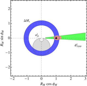
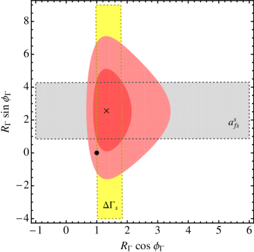
Figure 1: Left (Right): Constraints on $R_{M}$ and $\phi_{M}$ ($R_{\Gamma}$ and $\phi_{\Gamma}$) in scenario S1 (S2). For the individual constraints the colored areas are $68\%$ CL regions (${\rm dofs}=1$), while for the combined fit the red (light red) area is the $68\%$ ($95\%$) probability region (${\rm dofs}=2$). The SM values (best-fit solutions) are marked by a dot (cross).    

The four real parameters $R_{M,\Gamma}$ and $\phi_{M,\Gamma}$ entering (LABEL:eq:M12G12paraNP) can be constrained by confronting the observed values of $\Delta M_{s}$, $\phi_{J/\psi\phi}^{s}$, $\Delta\Gamma_{s}$, and $a_{fs}^{s}$ with their SM predictions. We begin our analysis by asking how well the SM hypothesis describes the data. Performing a global fit, we obtain $\chi^{2}=3.5$ corresponding to $0.7\sigma$ ($1.4\sigma$) for 4 (2) degrees of freedom (dofs). For the best-fit solution, we find instead $(R_{M},\phi_{M},R_{\Gamma},\phi_{\Gamma})=(1.02,2^{\circ},2.9,65^{\circ})$. After marginalization the corresponding symmetrized 68% CL parameter ranges are

$$R_{M} =1.04\pm 0.16\,, \qquad\phi_{M} =(-0.4\pm 5.0)^{\circ}\,,$$ (12)

$$R_{\Gamma} =3.4\pm 1.8\,, \qquad\phi_{\Gamma} =(56\pm 22)^{\circ}\,.$$

Focusing on $R_{\Gamma}$ and $\phi_{G}$, we see that a very good fit requires excessive corrections to $\Gamma_{12}^{s}$.

In order to further elucidate the latter point, we analyse two orthogonal hypothesis of new physics in $B_{s}$–$\bar{B}_{s}$ oscillations, namely a scenario with $(M_{12}^{s})_{\rm NP}\neq 0$ and $(\Gamma_{12}^{s})_{\rm NP}=0$ and a scenario with $(M_{12}^{s})_{\rm NP}=0$ and $(\Gamma_{12}^{s})_{\rm NP}\neq 0$. The left (right) panel in Figure 1 shows the results of our global fit for scenario S1 (S2) in the $R_{M}\hskip 0.7113pt\cos\phi_{M}$–$R_{M}\hskip 0.7113pt\sin\phi_{M}$ ($R_{\Gamma}\hskip 0.7113pt\cos\phi_{\Gamma}$–$R_{\Gamma}\hskip 0.7113pt\sin\phi_{\Gamma}$) plane. From the left panel, we glean that in the scenario S1 the regions of all individual constraints apart from $a_{fs}^{s}$ overlap. Minimizing the $\chi^{2}$ function gives $(R_{M},\phi_{M})=(1.03,2.0^{\circ})$ and $\chi^{2}/{\rm dofs}=3.4/2$ corresponding to $1.3\sigma$, which represents only a marginal improvement with respect to the SM hypothesis.$\!{}^{{\bf?},{\bf?}}$ In consequence, the case for a non-zero non-standard contribution to $M_{12}^{s}$ is rather weak. By inspection of the right panel, we see that in contrast to S1, in the scenario S2 a description of the data with a probability of better than 68% is possible. The best-fit point is located at $(R_{\Gamma},\phi_{\Gamma})=(2.9,62^{\circ})$. In fact, the latter parameters lead to an almost perfect fit with $\chi^{2}/{\rm dofs}=0.2/2$ corresponding to $0.1\sigma$. The data hence statistically favors the new-physics scenario S2 over the hypothesis S1.

3 New Physics in $b\to s\tau^{+}\tau^{-}$

The above findings suggest that one hypothetical explanation of the experimentally observed large negative values of $a_{fs}^{s}$ (or equivalent $A_{\rm SL}^{b}$) consists in postulating new physics in $\Gamma_{12}^{s}$ that changes the SM value by a factor of 3 or more. In the following we will study whether or not and to which extend such an speculative option is viable. While in principle any composite operator $(\bar{s}b)\hskip 0.7113ptf$, with $f$ leading to an arbitrary flavor neutral final state of at least two fields and total mass below the $B_{s}$-meson mass, can contribute to $\Gamma_{12}^{s}$, the field content of $f$ is in practice very restricted, since $B_{s}\to f$ and $B_{d}\to X_{s}\hskip 0.7113ptf$ decays to most final states involving light particles are severely constrained. One notable exception is the subclass of $B_{s}$- and $B_{d}$-meson decays to a pair of tau leptons, as has been first pointed out a few years ago.$\!{}^{{\bf?}}$

The possibility of large $b\to s\tau^{+}\tau^{-}$ contributions to $\Gamma_{12}^{s}$, can be analyzed in a model-independent fashion$\!{}^{{\bf?}}$ by adding

$${\cal L}_{\rm eff}=\frac{4G_{F}}{\sqrt{2}}\,V_{ts}^{\ast}V_{tb}\,\sum_{i}C_{i}(\mu)\,Q_{i}\,,$$ (13)

to the effective $\Delta B=1$ SM Lagrangian. Here $\mu$ denotes the renormalization scale and the Fermi constant $G_{F}$ as well as the leading Cabibbo-Kobayashi-Maskawa (CKM) factor $V_{ts}^{\ast}V_{tb}$ have been extracted as global prefactors. The index $i$ runs over the complete set of dimension-six operators with flavor content $(\bar{s}b)(\bar{\tau}\tau)$, namely ($A,B=L,R$)

$$\begin{split}Q_{S,AB}&=\left(\bar{s}\,P_{A}\,b\right)\left(\bar{\tau}\,P_{B}\,\tau\right)\,,\\ Q_{V,AB}&=\left(\bar{s}\,\gamma^{\mu}P_{A}\,b\right)\left(\bar{\tau}\,\gamma_{\mu}P_{B}\,\tau\right)\,,\\ Q_{T,A}&=\left(\bar{s}\,\sigma^{\mu\nu}P_{A}\,b\right)\left(\bar{\tau}\,\sigma_{\mu\nu}P_{A}\,\tau\right)\,,\end{split}$$ (14)

where $P_{L,R}=(1\mp\gamma_{5})/2$ project onto left- and right-handed chiral fields and $\sigma^{\mu\nu}=i\left[\gamma^{\mu},\gamma^{\nu}\right]/2$.

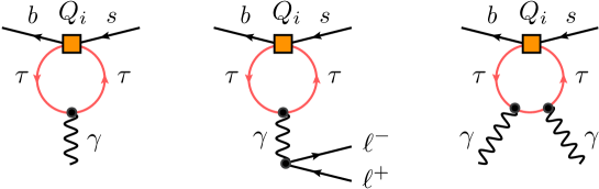
Figure 2: One-loop diagrams with a penguin insertion of a $(\bar{s}b)(\bar{\tau}\tau)$ operator (orange squares) that contribute to the processes $b\to s\gamma$ (left), $b\to s\ell^{+}\ell^{-}$ (middle), and $b\to s\gamma\gamma$ (right). The tau loop in all graphs is closed.    

The ten operators entering (14) govern the purely leptonic $B_{s}\to\tau^{+}\tau^{-}$ decay, the inclusive semi-leptonic $B\to X_{s}\tau^{+}\tau^{-}$ decay, and its exclusive counterpart $B^{+}\to K^{+}\tau^{+}\tau^{-}$, making these channels potentially powerful constraints. In practice, however, flavor-changing neutral current $B_{s,d}$ decays into final states involving taus are experimentally still largely unexplored territory, so that these direct constraints turn out to be not very strong. Explicitly, one obtains

$$\begin{split}{\cal B}(B_{s}\to\tau^{+}\tau^{-})\,&<\,3\%\,,\\ {\cal B}(B\to X_{s}\tau^{+}\tau^{-})\,&\lesssim\,2.5\%\,,\\ {\cal B}(B^{+}\to K^{+}\tau^{+}\tau^{-})\,&<\,3.3\cdot 10^{-3}\,.\end{split}$$ (15)

Here the first limit derives$\!{}^{{\bf?}}$ from comparing the SM prediction $\tau_{B_{s}}/\tau_{B_{d}}-1\in[-0.4,0.0]\%\;$$\!{}^{{\bf?}}$ with the corresponding experimental result $\tau_{B_{s}}/\tau_{B_{d}}-1=(0.4\pm 1.9)\%$, while the second (crude) bound follows from estimating$\!{}^{{\bf?}}$ the possible contamination of the exclusive and inclusive semileptonic decay samples by $B\to X_{s}\tau^{+}\tau^{-}$ events. Limits on ${\cal B}(B_{s}\to\tau^{+}\tau^{-})$ and ${\cal B}(B\to X_{s}\tau^{+}\tau^{-})$ of strength similar to those given in (15) also follow from charm counting$\!{}^{{\bf?}}$ and/or LEP searches for $B$ decays with large missing energy.$\!{}^{{\bf?}}$ The final number corresponds to the 90% CL upper limit on the branching ratio of $B^{+}\to K^{+}\tau^{+}\tau^{-}$ as measured by BaBar.$\!{}^{{\bf?}}$

Further constraints on the Wilson coefficients of the $(\bar{s}b)(\bar{\tau}\tau)$ operators arise indirectly from the experimentally available information on the $b\to s\gamma$, $b\to s\ell^{+}\ell^{-}$ ($\ell=e,\mu$), and $b\to s\gamma\gamma$. transitions, because some of the effective operators introduced in (14) mix into the electromagnetic dipole operators $Q_{7,A}$ and the vector-like semileptonic operators $Q_{9,A}$. The relevant Feynman diagrams are shown in Figure 2. An explicit calculation$\!{}^{{\bf?}}$ shows that the operators $Q_{S,AB}$ mix neither into $Q_{7,A}$ nor $Q_{9,A}$, while $Q_{V,AB}$ ($Q_{T,A}$) mixes only into $Q_{9,A}$ ($Q_{7,A}$). As a result of the particular mixing pattern, the stringent constraints from the radiative decay $B\to X_{s}\gamma$ rule out large contributions to $\Gamma_{12}^{s}$ only if they arise from the tensor operators $Q_{T,A}$. Similarly, the rare decays $B\to X_{s}\ell^{+}\ell^{-}$ and $B\to K^{(\ast)}\ell^{+}\ell^{-}$ primarily limit contributions stemming from the vector operators $Q_{V,AB}$. In contrast to $B\to X_{s}\gamma$, all $(\bar{s}b)(\bar{\tau}\tau)$ operators contribute to the double-radiative $B_{s}\to\gamma\gamma$ decay at the one-loop level. A detailed study$\!{}^{{\bf?}}$ shows however that the limits following from $b\to s\gamma\gamma$ are in practice not competitive with the bounds obtained from the other tree- and loop-level mediated $B_{s,d}$-meson decays.

Operator	Bound on $C_{i}(m_{b})$	Bound on $\Lambda$	Observable
$(\bar{s}\,P_{A}\,b)(\bar{\tau}\,P_{B}\,\tau)$	0.5	$2.0{\rm\;TeV}$	$B_{s}\to\tau^{+}\tau^{-}$
$(\bar{s}\,\gamma^{\mu}P_{A}\,b)(\bar{\tau}\,\gamma_{\mu}P_{B}\,\tau)$	0.8	$1.0{\rm\;TeV}$	$B^{+}\to K^{+}\tau^{+}\tau^{-}$
$(\bar{s}\,\sigma^{\mu\nu}P_{L}\,b)(\bar{\tau}\,\sigma_{\mu\nu}P_{L}\,\tau)$	0.06	$3.2{\rm\;TeV}$	$B\to X_{s}\gamma$
$(\bar{s}\,\sigma^{\mu\nu}P_{R}\,b)(\bar{\tau}\,\sigma_{\mu\nu}P_{R}\,\tau)$	0.09	$2.8{\rm\;TeV}$	$B\to X_{s}\gamma$

Table 1: Model-independent limits on the Wilson coefficients of $(\bar{s}b)(\bar{\tau}\tau)$ operators. The second (third) column shows the limit on $C_{i}(m_{b})$ (the bound on the suppression scale $\Lambda$ assuming a coupling strength of 1).

The model-independent 90% CL limits on the magnitudes of the Wilson coefficients are summarized in Table 1. We see that in the case of the $(\bar{s}b)(\bar{\tau}\tau)$ scalar and vector operators the allowed effects can reach almost ${\cal O}(1)$. These Wilson coefficients can hence be similar in size to that of the color-singlet current-current operator $Q_{2}$, which provides the dominant contribution to $\Gamma_{12}^{s}$ in the SM. In consequence, the corresponding suppression scale $\Lambda$ is quite low, around $(1-2)\,{\rm TeV}$. Possible new-physics contributions to the $(\bar{s}b)(\bar{\tau}\tau)$ tensor operators are more severely constrained, because they lead to a contamination of $B\to X_{s}\gamma$. It is also interesting to ask which impact future improved extractions of ${\cal B}(B_{s}\to\tau^{+}\tau^{-})$, ${\cal B}(B\to X_{s}\tau^{+}\tau^{-})$, and ${\cal B}(B^{+}\to K^{+}\tau^{+}\tau^{-})$ will have on the limits on the Wilson coefficients $C_{i}(m_{b})$. Such a comparison is provided in Figure 3. From the left panel one concludes that ${\cal B}(B^{+}\to K^{+}\tau^{+}\tau^{-})<1.3\cdot 10^{-3}$, corresponding to an improvement of the present upper limit by a factor of 2.5, would allow to set a bound on $C_{S,A}(m_{b})$ that is as good as the one that follows at present already from $B_{s}\to\tau^{+}\tau^{-}$. As can seen from the right panel, in the case of $C_{V,AB}(m_{b})$, limits of ${\cal B}(B_{s}\to\tau^{+}\tau^{-})<1.7\%$ and ${\cal B}(B\to X_{s}\tau^{+}\tau^{-})<0.7\%$ are needed to be competitive with $B^{+}\to K^{+}\tau^{+}\tau^{-}$. The quoted limits correspond to improvements of our current knowledge of the relevant $B$-meson branching ratios by a factor of 1.8 and 3.6, respectively. Finally, for what concerns $C_{T,A}(m_{b})$, even improvements of the direct constraints by a factor of more than 10 are not sufficient to beat the indirect constraint arising from $B\to X_{s}\gamma$.

4 Effects of $(\bar{s}b)(\bar{\tau}\tau)$ Operators in $\Gamma_{12}^{s}$

The off-diagonal element of the decay-width matrix is related via the optical theorem to the absorptive part of the forward-scattering amplitude which converts a $\bar{B}_{s}$ into a $B_{s}$ meson. Working to leading order in the strong coupling constant and $\Lambda_{\rm QCD}/m_{b}$, the contributions from the complete set of operators (14) to $\Gamma_{12}^{s}$ is found by computing the matrix elements of the $(Q_{i},Q_{j})$ double insertions between quark states. Such a calculation$\!{}^{{\bf?}}$ leads to the results

$$\begin{split}(R_{\Gamma})_{S,AB}&<1+\left(0.4\pm 0.1\right)|C_{S,AB}(m_{b})|^{2}\,,\\[5.69054pt] (R_{\Gamma})_{V,AB}&<1+\left(0.4\pm 0.1\right)|C_{V,AB}(m_{b})|^{2}\,,\\[5.69054pt] (R_{\Gamma})_{T,A}&<1+\left(3.6\pm 0.9\right)|C_{T,A}(m_{b})|^{2}\,,\end{split}$$ (16)

where the quoted uncertainties are due to the error on $(\Delta\Gamma_{s})_{\rm SM}$ as given in (4). Employing now the 90% CL bounds on the low-energy Wilson coefficients given in Table 1, it follows that

$$(R_{\Gamma})_{S,AB}<1.15\,,\qquad(R_{\Gamma})_{V,AB}<1.35\,,\qquad(R_{\Gamma})_{T,L}<1.02\,,\qquad(R_{\Gamma})_{T,R}<1.04\,.$$ (17)

These numbers imply that $(\bar{s}b)(\bar{\tau}\tau)$ operators of scalar (vector) type can lead to enhancements of $|\Gamma_{12}^{s}|$ over its SM value by 15% (35%) without violating any existing constraint. In contrast, contributions from tensor operators can alter $|\Gamma_{12}^{s}|$ by at most $4\%$. These numbers should be compared to the best-fit solution for $R_{\Gamma}$ as given in (12). From the comparison it immediately becomes apparent that absorptive new physics in $\Gamma_{12}^{s}$ in form of $(\bar{s}b)(\bar{\tau}\tau)$ operators cannot provide a satisfactory explanation of the anomaly in the dimuon charge asymmetry data observed by the DØ collaboration. This is a model-independent conclusion that can be shown to hold in explicit models of new physics with modification of the $b\to s\tau^{+}\tau^{-}$ channel such as leptoquark scenarios or $Z^{\prime}$ models.$\!{}^{{\bf?}}$

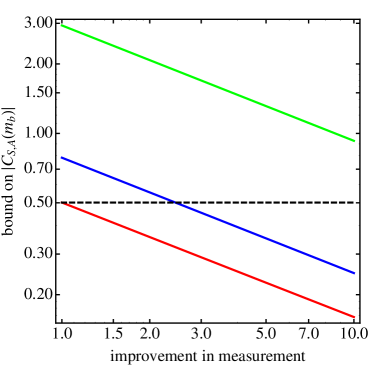
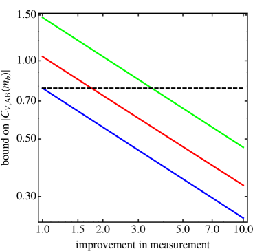
Figure 3: Left (Right): Bound on $C_{S,A}(m_{b})$ ($C_{V,AB}(m_{b})$) from improved determinations of ${\cal B}(B_{s}\to\tau^{+}\tau^{-})$ (red), ${\cal B}(B\to X_{s}\tau^{+}\tau^{-})$ (green), and ${\cal B}(B^{+}\to K^{+}\tau^{+}\tau^{-})$ (blue). The dashed lines indicate the presently best bound.  

5 Conclusions and Outlook

Motivated by the observation that the anomalously large dimuon charge asymmetry measured by the DØ collaboration, can be fully explained only if new physics contributes to the absorptive part of the $B_{s,d}$–$\bar{B}_{s,d}$ mixing amplitudes, we have presented a model-independent study of the contributions to $\Gamma_{12}^{s}$ arising from the complete set of dimension-six $(\bar{s}b)(\bar{\tau}\tau)$ operators. Taking into account the direct bounds from $B_{s}\to\tau^{+}\tau^{-}$, $B\to X_{s}\tau^{+}\tau^{-}$, and $B^{+}\to K^{+}\tau^{+}\tau^{-}$ as well as the indirect constraints from $b\to s\gamma$, $b\to s\ell^{+}\ell^{-}$, and $b\to s\gamma\gamma$, we have demonstrated that only the Wilson coefficients of the tensor operators are severely constrained by data, while those of the scalar and vector operators can be sizable and almost reach the size of the Wilson coefficient of the leading current-current SM operator. It follows that the presence of a single $(\bar{s}b)(\bar{\tau}\tau)$ operator can lead to an enhancement of $\Gamma_{12}^{s}$ of at most 35% compared to its SM value. Since a resolution of the tension in the $B_{s}$-meson sector would require the effects to be of the order of 300% (or larger), the allowed shifts are by far too small to provide an satisfactory explanation of the issue. We emphasize that after minor modifications, our general results can be applied to other dimension-six operators involving quarks and leptons. For example, as a result of the 90% CL limit ${\cal B}(B^{+}\to K^{+}\tau^{\pm}\mu^{\mp})<7.7\cdot 10^{-5}$,$\!{}^{{\bf?}}$ the direct bounds on the Wilson coefficients of the set of $(\bar{s}b)(\bar{\tau}\mu)$ operators turn out to be roughly a factor of $7$ stronger than those in the $(\bar{s}b)(\bar{\tau}\tau)$ case. Possible effects of $(\bar{s}b)(\bar{\tau}\mu)$ operators are therefore generically too small to lead to a notable improvement of the tension present in the current $B_{s,d}$-meson data. Similarly, a contribution from $(\bar{d}b)(\bar{\tau}\tau)$ operators to $\Gamma_{12}^{d}$ large enough to explain the $A_{\rm SL}^{b}$ data is excluded by the 90% CL bound ${\cal B}(B\to\tau^{+}\tau^{-})<4.1\cdot 10^{-3}$.$\!{}^{{\bf?}}$ Naively, also $(\bar{b}d)(\bar{c}c)$ operators are heavily constrained (meaning that their Wilson coefficients should be smaller than those of the QCD/electroweak penguins in the SM) by the plethora of exclusive $B$ decays. A dedicated analysis of the latter class of contributions is however not available in the literature.

Our model-independent study of non-standard effects in $\Gamma_{12}^{s}$ can readily be applied to explicit SM extensions involving leptoquarks or $Z^{\prime}$ bosons. In fact, the pattern of deviations found in these scenarios resembles the one of all new-physics model with real $r_{\rm NP}=(M_{12}^{s})_{\rm NP}/(\Gamma_{12}^{s})_{\rm NP}$, for which it can be shown that the measurement of $\Delta M_{s}$ generically puts stringent constraints on both $\Delta\Gamma_{s}$ and $a_{fs}^{s}$. These bounds turn out to be weakest if the ratio $r_{\rm NP}$ is positive and as small as possible. Since on dimensional grounds $r_{\rm NP}$ scales as the square of the new-physics scale, this general observation implies that SM extensions that aim at a good description of the Tevatron data should have new degrees of freedom below the electroweak scale and/or be equipped with a mechanism that renders the contribution to $M_{12}^{s}$ small. Furthermore, models in which $(M_{12}^{s})_{\rm NP}$ is generated beyond Born level seem more promising, since in such a case $r_{\rm NP}$ is suppressed by a loop factor with respect to the case where $(M_{12}^{s})_{\rm NP}$ arises already at tree level.

The above discussion implies that a full explanation of the observed discrepancies is not even possible for the most general case $(M_{12}^{s})_{\rm NP}\neq 0$ and $(\Gamma_{12}^{s})_{\rm NP}\neq 0$. Numerically, one finds that the addition of a single $(\bar{s}b)(\bar{\tau}\tau)$ vector operator giving $(R_{\Gamma})_{V,AB}=1.35$ on top of dispersive new physics with $(M_{12}^{s})_{\rm NP}\neq 0$, can only improve the quality of the fit to the latest set of measurements to $\chi^{2}=1.4$ compared to $\chi^{2}=3.5$ within the SM. This might indicate that the high central value of $A_{\rm SL}^{b}$ observed by the DØ collaboration is (partly) due to a statistical fluctuation. Future improvements in the measurement of the CP phase $\phi_{J/\psi\phi}^{s}$ and, in particular, a first determination of the difference $a_{fs}^{s}-a_{fs}^{d}$ between the $B_{s}$ and $B_{d}$ semileptonic asymmetries by LHCb, are soon expected to shed light on this issue, and are of utmost importance in order to answer whether or not there is new physics hiding in the $B_{s,d}$-meson sector.

References

• [1] A. Abulencia et al. [CDF Collaboration], Phys. Rev. Lett.  97, 242003 (2006) [hep-ex/0609040].
• [2] R. Aaij et al. [LHCb Collaboration], Phys. Lett. B 709, 177 (2012) [arXiv:1112.4311 [hep-ex]].
• [3] A. Lenz, arXiv:1205.1444 [hep-ph] and references therein.
• [4] P. Clarke, LHCb-TALK-2012-029, http://cdsweb.cern.ch/record/1429149/files/LHCb-TALK-2012-029.pdf
• [5] V. M. Abazov et al. [DØ Collaboration], Phys. Rev. D 84, 052007 (2011) [arXiv:1106.6308 [hep-ex]].
• [6] D. Asner et al. [Heavy Flavor Averaging Group], arXiv:1010.1589 [hep-ex], updated results available at http://www.slac.stanford.edu/xorg/hfag/
• [7] C. Bobeth and U. Haisch, arXiv:1109.1826 [hep-ph].
• [8] A. Dighe, A. Kundu and S. Nandi, Phys. Rev. D 76, 054005 (2007) [arXiv:0705.4547 [hep-ph]].
• [9] A. Dighe, A. Kundu and S. Nandi, Phys. Rev. D 82, 031502 (2010) [arXiv:1005.4051 [hep-ph]].
• [10] A. L. Kagan and J. Rathsman, hep-ph/9701300.
• [11] Y. Grossman, Z. Ligeti and E. Nardi, Phys. Rev. D 55, 2768 (1997) [hep-ph/9607473].
• [12] K. Flood [BaBar Collaboration], PoS ICHEP2010, 234 (2010).
• [13] B. Aubert et al. [BaBar Collaboration], Phys. Rev. Lett.  99, 201801 (2007) [arXiv:0708.1303 [hep-ex]].
• [14] B. Aubert et al. [BABAR Collaboration], Phys. Rev. Lett.  96, 241802 (2006) [hep-ex/0511015].