Fracturing highly disordered materials

Abstract

We investigate the role of disorder on the fracturing process of heterogeneous materials by means of a two-dimensional fuse network model. Our results in the extreme disorder limit reveal that the backbone of the fracture at collapse, namely the subset of the largest fracture that effectively halts the global current, has a fractal dimension of $1.22\pm 0.01$. This exponent value is compatible with the universality class of several other physical models, including optimal paths under strong disorder, disordered polymers, watersheds and optimal path cracks on uncorrelated substrates, hulls of explosive percolation clusters, and strands of invasion percolation fronts. Moreover, we find that the fractal dimension of the largest fracture under extreme disorder, $d_{f}=1.86\pm 0.01$, is outside the statistical error bar of standard percolation. This discrepancy is due to the appearance of trapped regions or cavities of all sizes that remain intact till the entire collapse of the fuse network, but are always accessible in the case of standard percolation. Finally, we quantify the role of disorder on the structure of the largest cluster, as well as on the backbone of the fracture, in terms of a distinctive transition from weak to strong disorder characterized by a new crossover exponent.

The brittle fracture of heterogeneous systems still represents a major challenge from both scientific and technological points of view. It has been the subject of intense scientific research in physics, material science, mechanical and metallurgical engineering Marder2010 ; Kanninen1985 ; Sahimi1998 ; Alava2006 . The amount of small cracks and the shape of the largest fracture potentially determine whether or not the system still supports external loads and how catastrophic will be the rupture. Previous studies have shown that the degree of disorder in the material rules the transition between abrupt and gradual ruptures, i.e., the more heterogeneous is the material, more warnings one gets before the system collapses Herrmann1988 . However, the nature of this transition, as well as the behavior of the fracturing system in the limit of strong disorder Malakhovsky2007 ; Hao2012 , remain as important open questions. Evidently, to model fracturing formation, it is fundamental to determine how stress is redistributed over the system while cracks appear, grow, and merge. Although conceptually simple, the fuse network model is a good candidate for dealing with such problem, since it can clearly capture the essential features of the involved physical phenomena. In this model, resistors are used to mimic springs, in an approximate description for elasticity, where vector and tensor fields describing fracture mechanics are replaced by a scalar field representing the local strain Hansen1991 ; Arcangelis1989 ; Gilabert1987 ; Zapperi2008 .

The purpose of this Letter is to investigate the role of disorder on the scaling properties of the fuse network model at the critical collapse condition. We first study in detail the limiting case of extreme disorder. This is performed by measuring, through a purely geometrical technique, the fractal dimension of three different structures, namely the backbone of the fracture of broken bonds that halts current through the lattice, the largest fracture formed by the broken bonds (backbone plus dangling ends attached to it), and the total network of all broken bonds (largest cluster plus smaller clusters not attached to it). We then show how the self-similar behavior of the resulting fracture topology crosses over from one regime to another as we move from weak to strong disorder.

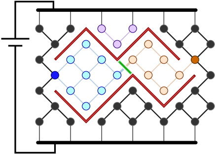
Figure 1: (Color online) The fuse network under extreme disorder. In each step, a random bond belonging to the conducting part of the network is chosen to burn. Here the burnt bonds were removed and the red lines placed instead, but in the complementary lattice. The red lines represent cracks in the system and the green line close to the middle of the panel corresponds to a bond that will merge two large cracks, forming two cavities in the lattice (light blue and yellow dots). Since the current can not go through, none of the bonds inside the cavities (light blue and yellow lines) can burn in the next steps. The dark blue and brown dots depict the limiting boundaries of each cavity. Note that the resulting fracture forms no loops. The purple dots in the middle top of the lattice correspond to sites connected to only one of the poles, therefore they do not participate in the transport, and the (purple) bonds connected to them do not burn either.

Let us start by describing the fuse network model Arcangelis1985 ; Herrmann1988 . In the traditional version of this model, the electric potential in a resistor network should provide a simplified description of the local strain in a fracturing system. A crack forms when the stress or, correspondingly, the electric current over a given resistor, surpasses a certain threshold. Therefore, our system is a lattice where each bond is a resistor with a given conductance and fusing threshold value. For simplicity, we consider here the case in which the conductance is the same for all bonds, however, we expect similar results with a varying conductance footnote1 . We model the heterogeneity by assigning to each bond $i$ a threshold given by $\tau_{i}=10^{\beta R_{i}}$, where $R_{i}$ is a random number uniformly distributed in the interval $-1<R_{i}<1$. Therefore, the distribution of thresholds is hyperbolic, $P_{\tau}(\tau)\sim\tau^{-1}$, with upper and lower bounds given by $10^{\beta}$ and $10^{-\beta}$, respectively.

Generally speaking, we consider that a potential difference is applied between two opposite sides of a resistor network, and solve Kirchhoff’s law to determine the current passing through each bond HSL . Below the threshold value, each bond conducts according to Ohm’s law, but once the current $I_{i}$ at a given bond $i$ reaches the threshold $\tau_{i}$, the bond burns (or breaks, in the mechanical terminology) and becomes an insulator. In this way, the largest current-threshold ratio, $max(I_{i}/\tau_{i})$, determines the next bond to be burnt. Here we assume that the potential starts from zero and raises slowly, allowing only one bond to burn at each step. Pathological defects in the system are avoided by using a tilted square lattice, therefore in the first step all currents are the same, and the bond with the smaller threshold is the first to burn. In the following steps, inhomogeneities are gradually introduced in the system due to the burnt bonds, so that local threshold and current values should determine which one burns next.

We initially focus on the case of a fuse network under extreme disorder, $\beta\to\infty$, where thresholds are distributed over many orders of magnitude. In this limit, for all practical purposes, one can assume that the smaller (larger than one) ratio between the thresholds of any two bonds in the lattice is larger than the largest ratio of the currents of any two bonds that constitute the conducting part of the network. In this regime, any variability in the currents becomes irrelevant so that the next bond to burn should be the one with the smaller threshold among those that participate in transport. Since the thresholds are randomly distributed over the lattice, this is entirely equivalent to a process in which a random bond with finite current, $I>0$, is chosen to burn at each step. As the bonds burn, however, they may form a cavity that is connected to the rest of the lattice at a single node, as represented in Fig. 1. Because all nodes inside a cavity are equipotential, their connecting bonds are current-free and can not burn, regardless of their thresholds.

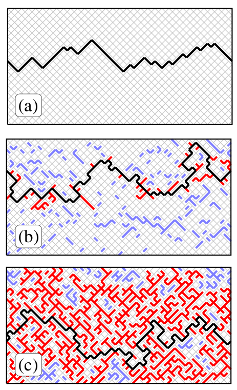
Figure 2: (Color online) Typical realizations of the fuse network at the point of disconnection ($L=32$). In (a) $\beta=0.01$ (weak disorder); in (b) $\beta=1$ (intermediate disorder); and in (c) $\beta=100$ (strong disorder, for this lattice size). As represented in Fig. 1, the fractures occupy the‘ places of the burnt bonds, but in the complementary lattice. The black lines show the backbone with mass $M_{b}$, namely the number of burnt bonds forming the chain that effectively disconnects the bottom from the top of system. The set of all cracks connected to form the largest fracture, namely the backbone and its dangling ends (black and red lines, respectively) have mass $M_{f}$, while $M_{t}$ denotes the total mass, i.e., the mass of the largest fracture plus all the other cracks (light blue lines) in the system.

In this way, the extreme disorder limit of the fuse network model can be viewed as a modified percolation problem. In the standard percolation, bonds are randomly and sequentially occupied, while in the fuse network under extreme disorder, one only burns (occupies) bonds that belong to the conducting backbone of the lattice. As shown in Fig. 1, once a cavity is formed, the bonds inside remain unoccupied and, as a consequence, the clusters of occupied bonds in the complementary lattice do not form loops. Under this reasoning, the extreme disorder limit of the fuse network model becomes a purely geometrical problem. Simulations performed with fuse networks at $\beta=10^{8}$ confirm that these two models are identical. Such a geometrical approach for the extreme disorder case greatly reduces the computational demand of the problem, therefore enabling us to simulate the fracturing process for networks with linear size $L$ going from $16$ to $2048$, and using at least $1000$ samples for the largest size. As shown in Fig. 2, we stop each realization when the two sides, where the potential difference is applied, become disconnected, i.e., no current can pass through the system.

In Fig. 3 we show that the mass of the largest fracture, $M_{f}$, its backbone mass $M_{b}$, as well as the set of all broken bonds, $M_{t}$, grow with the system size as power laws. First, the total mass of burnt bonds scales with the linear size as, $M_{t}\sim{L^{d_{t}}}$, with $d_{t}=2.00\pm{0.01}$, suggesting that the bonds burn homogeneously through the lattice. The backbone grows as $M_{b}\sim{L^{d_{b}}}$, with $d_{b}=1.22\pm{0.01}$, which is statistically identical to the exponent obtained for optimal paths under strong disorder Andrade2009 , disordered polymers Cieplak1994 , watersheds Fehr2009 and optimal path cracks on uncorrelated substrates Oliveira2011 , the hulls of explosive percolation clusters Araujo2010 , and the strands of invasion percolation fronts Cieplak1996 . For the largest fracture, however, we obtain $M_{f}\sim{L^{d_{f}}}$, with $d_{f}=1.86\pm{0.01}$, which is different from the fractal dimension of the largest cluster in 2D percolation, $d_{p}=1.8958$ Stauffer1992 ; Roux1988 .

In the limit of extreme disorder, the fracture backbone in the fuse model is identical to the one of loopless percolation Porto1997 . This can be seen by considering that the burning of fuses of a specific configuration of thresholds due to the extreme disorder just follows the sequence of their inverse rank, except if the fuse would close a loop or lie inside a nearly closed loop. In parallel, one can construct a configuration of loopless percolation by assigning an occupation rank to each site of the lattice identical to the ranking given by the thresholds (and obviously not occupying a site which would close a loop). The spanning cluster of this percolation configuration then consists of the fracture of the fuse model and sites inside nearly closed loops that do not contribute to the backbone. This shows that the bonds forming the backbone should be exactly the same in both models. It was previously observed that the backbone of loopless percolation has the same fractal dimension as the optimum path in strong disorder Schrenk2012 , therefore giving support to this argument.

The cavities can not change the fractal dimension of the backbone but may very well change the dimension of the largest fracture. The largest fracture comprises the backbone and the dangling ends attached to it. Once a cavity is formed in the largest fracture, it precludes the growing and attaching of other dangling ends inside it. As a consequence, the largest fracture in the extreme disorder fuse model is certainly smaller than the largest cluster in standard percolation. Since we obtain, for the former case, a fractal dimension smaller than the expected for standard percolation, we conclude that cavities form at every scale, and the difference between the two models becomes increasingly relevant as the system size grows.

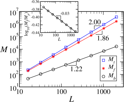
Figure 3: (Color online) Size dependence results obtained for the fuse network model under extreme disorder. The total number of burnt bonds in the system scales as, $M_{t}\sim{L^{d_{t}}}$, with $d_{t}=2.00\pm{0.01}$, indicating that the cracks appear homogeneously in the 2D lattice. The largest fracture for this model grows as $M_{f}\sim{L^{d_{f}}}$, with $d_{f}=1.86\pm{0.01}$, suggesting a different universality class for this structure than that of the spanning cluster in standard percolation Stauffer1992 . Finally, the mass of the backbone of the largest fracture scales as $M_{b}\sim{L^{d_{b}}}$, with $d_{b}=1.22\pm{0.01}$. The results shown in the inset confirm that the ratio between the masses of the largest clusters in the fuse and in the percolation models scales as, $M_{f}/M_{p}\sim{L^{d_{f}-d_{p}}}$, with $d_{f}-d_{p}\approx{-0.03}$.

To further test our hypothesis, we performed simulations with a pinpoint algorithm that builds simultaneously percolation clusters and fuse network fractures under extreme disorder. Precisely, at each step, we randomly choose a bond in the lattice and, if this bond is part of the conducting backbone, it is occupied in the percolation lattice as well as burnt in the fuse network. If this bond is inside one of the cavities, however, it is occupied only in the percolation lattice and not in the fuse network. Once a cluster forms that crosses the system, the percolation condition is achieved in both models simultaneously. If the fractal dimensions are in fact different, the ratio between the masses of the largest clusters, $M_{f}/M_{p}$, where $M_{p}$ is the mass of the spanning cluster in percolation, should vary with the system size as a power law, with an exponent given by $d_{f}-d_{p}\approx{-0.03}$. The obtained results shown in the inset of Fig. 3 support our conjecture that the largest fracture of the fuse network under extreme disorder corresponds to a subset of the spanning cluster in percolation. Moreover, this new object is also self-similar, but with a slightly smaller fractal dimension.

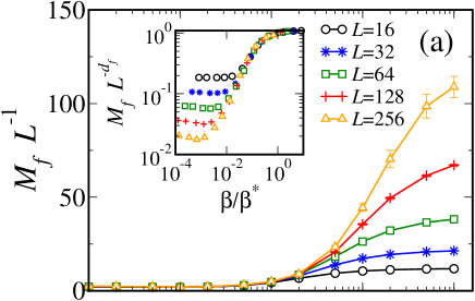
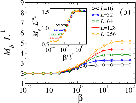
Figure 4: (Color online) The transition from weak to strong disorder. We show the mass of the largest fracture (a) and backbone (b) as function of the disorder parameter $\beta$. In the week disorder regime, $\beta<\beta^{*}$, we have a linear growth for both backbone and largest fracture. As $\beta$ increases the masses cross over for the strong disorder regime where a super-linear growth is observed. The exponents $d_{f}$ and $d_{b}$, controlling the scaling in the strong regime, are the same as in Fig (3). The value $\beta^{*}$ determining the onset of the crossover scales with the size of the system as $\beta^{*}\sim{L^{0.9}}$.

It is important to mention that some variants of the percolation model previously investigated also depart from the universality class of standard percolation. For example, in invasion percolation with trapping Wilkinson1983 , when a loop is formed in the growing cluster, no site or bond inside this loop can be occupied, constituting a trapped region. These trapped regions are somehow similar to our cavities, only that cavities are sections of the lattice outside the conducting backbone of unoccupied bonds, while trapped regions are sections outside the infinite cluster of unoccupied bonds. In this case, statistically relevant deviations have also be detected from the fractal dimension of the spanning cluster in standard percolation Roux89 ; Sheppard99 .

Next we investigate how the behavior of the fuse network model crosses over from weak to strong disorder by gradually increasing the value of the parameter $\beta$. Local currents are computed by applying Kirchhoff’s law to each site of the network at each burning step, and solving the resulting system of linear algebraic equations. In weak disorder, most of the burnt bonds belong to the backbone of the fracture that grows linearly with the system size, $d_{b}=d_{f}=1$. As $\beta$ increases, the fractal dimensions obtained in the extreme disorder limit should be eventually recovered. Figure 4 shows how the masses $M_{f}$ and $M_{b}$ vary with the disorder parameter $\beta$. For small values, $\beta<0.1$, both masses are proportional to the system size, and depend weakly on $\beta$. For intermediate values, $0.1<\beta<\beta^{*}(L)$, the masses depend of $\beta$ but still grow linearly with $L$, therefore indicating the persistence of the weak disorder regime. However, as one goes to larger values, $\beta>\beta^{*}(L)$, the curves cross over to the strong disorder regime, where the masses show super-linear growth with system size, $M_{t}\sim{L^{d_{t}}}$, $M_{f}\sim{L^{d_{f}}}$, and $M_{b}\sim{L^{d_{b}}}$, but are again not dependent on $\beta$. The value $\beta^{*}$ marks the transition from weak to strong disorder. One should expect that, above a characteristic length $\xi$, the system scales as in the weak disorder limit. Certainly, the length $\xi$ should depend on the strength of the disorder, diverging in the extreme disorder as $\xi\sim\beta^{\frac{1}{\eta}}$. The onset of the strong disorder regime takes place when $\xi>L$, resulting in $\beta^{*}\sim{L^{\eta}}$. The insets of Figs. 4 show the data scaled by the fractal dimensions and $\beta^{*}$, with the controlling exponent $\eta=0.9\pm 0.1$. The collapse of the curves in the transition region corroborates our analysis and reveals the presence of a crossover between the two regimes.

In conclusion, our results show that the threshold disorder introduces a characteristic scale $\xi$ in the system. Below this scale, the fracture backbone displays a tortuous self-similar shape, with the same fractal dimension of the optimum path under strong disorder Cieplak1994 ; Cieplak1996 and other previously investigated models Andrade2009 ; Fehr2009 ; Oliveira2011 ; Araujo2010 . For scales larger than $\xi$, the fractures grow linearly with system size, consistent with the weak disorder regime. In the limit of extreme disorder, $\xi\to\infty$, the largest fracture has a fractal dimension of $d_{f}=1.86\pm{0.01}$, close to, but different from the fractal dimension of percolation clusters Roux1988 .

We thank the Brazilian Agencies CNPq, CAPES, FUNCAP and FINEP, the FUNCAP/CNPq Pronex grant, and the National Institute of Science and Technology for Complex Systems in Brazil for financial support.

References

- (1) M. P. Marder, Condensed Matter Physics - second edition (Wiley, New Jersey, 2010).
- (2) M. F. Kanninen and C. H. Popelar, Advanced Fracture Mechanics (The Oxford Engineering Science Series, New York, 1985).
- (3) M. Sahimi, Physics Reports 306, 213 (1998).
- (4) M. J. Alava, P. K. V. V. Nukala, and S. Zapperi, Adv. Phys. 55, 349 (2006).
- (5) B. Kahng, G. G. Batrouni, S. Redner, L. de Arcangelis, and H. J. Herrmann, Phys. Rev. B 37, 37 (1988).
- (6) I. Malakhovsky and M. A. J. Michels, Phys. Rev. B 76, 144201 (2007).
- (7) D.-P. Hao, G. Tang, H. Xia, K. Han, and Z.-P. Xun, J. Stat. Phys. 146, 1203 (2012).
- (8) A. Hansen, E. L. Hinrichsen, and S. Roux, Phys. Rev. Lett. 66, 2476 (1991); A. Hansen, E. L. Hinrichsen, and S. Roux, Phys. Rev. B 43, 665 (1991).
- (9) L. de Arcangelis, A. Hansen, H. J. Herrmann, and S. Roux, Phys. Rev. B 40, 877 (1989).
- (10) A. Gilabert, C. Vanneste, D. Sornette, and E. Guyon, J. Physique 48, 763 (1987).
- (11) M. J. Alava, P. K. V. V. Nukala, and S. Zapperi, Int. J. Fract. 154, 51 (2008); P. K. V. V. Nukala, S. Zapperi, M. J. Alava, and S. Šimunović, Int. J. Fract. 154, 119 (2008); C. Manzato, A. Shekhawat, P. K. V. V. Nukala, M. J. Alava, J. P. Sethna, and S. Zapperi, Phys. Rev. Lett. 108, 065504 (2012).
- (12) L. de Arcangelis, S. Redner, and H. J. Herrmann, J. Physique Lett. 46, L-585 (1985).
- (13) In the case where all the conductances are the same, some symmetric conditions may happen, where a fraction of the backbone lies on a Wheatstone bridge connecting sites with the same potential. Our geometrical model does not account for this possibility. However, we performed tests introducing disorder in the conductance, apart from the disorder in the thresholds, avoiding this effect, and obtained similar results. In fact, no qualitative difference is expected, as long as the distribution of conductance is bounded, not ranging over many order of magnitudes.
- (14) The linear equation system was solved through the HSL library, a collection of FORTRAN codes for large-scale scientific computation. See http://www.hsl.rl.ac.uk/.
- (15) J. S. Andrade, E. A. Oliveira, A. A. Moreira, and H. J. Herrmann, Phys. Rev. Lett. 103, 225503 (2009).
- (16) M. Cieplak, A. Maritan, and J. R. Banavar, Phys. Rev. Lett. 72, 2320 (1994).
- (17) E. Fehr, J. S. Andrade, S. D. da Cunha, L. R. da Silva, H. J. Herrmann, D. Kadau, C. F. Moukarzel, and E. A. Oliveira, J. Stat. Mech. P09007 (2009).
- (18) E. A. Oliveira, K. J. Schrenk, N. A. M. Araújo, H. J. Herrmann, and J. S. Andrade, Phys. Rev. E 83, 046113 (2011).
- (19) N. A. M. Araújo and H. J. Herrmann, Phys. Rev. Lett. 105, 035701 (2010).
- (20) M. Cieplak, A. Maritan, and J. R. Banavar, Phys. Rev. Lett. 76, 3754 (1996).
- (21) D. Stauffer and A. Aharony, Introduction to Percolation Theory (Taylor & Francis, London, 1992).
- (22) S. Roux, A. Hansen, H. Herrmann, and E. Guyon, J. Stat. Phys. 52, 237 (1988).
- (23) M. Porto, S. Havlin, S. Schwarzer, and A. Bunde, Phys. Rev. Lett. 79, 4060 (1997); M. Porto, N. Schwartz, S. Havlin, and A. Bunde, Phys. Rev. E 60, R2448 (1999).
- (24) K. J. Schrenk, N. A. M. Araújo, J. S. Andrade, and H. J. Herrmann, Sci. Rep. 2, 348 (2012).
- (25) D. Wilkinson and J. F. Willemsen, J. Phys. A 16, 3365 (1983).
- (26) S. Roux and E. Guyon, J. Phys. A 22, 3693 (1989).
- (27) A. P. Sheppard, M. A. Knackstedt, W. V. Pinczewski, and M. Sahimi, J. Phys. A 32, L521 (1999).