The non-Abelian Duality Problem

Abstract

We exploit a new theory of duality transformations to construct dual representations of models incompatible with traditional duality transformations. Hence we obtain a solution to the long-standing problem of non-Abelian dualities that hinges on two key observations: (i) from the point of view of dualities, whether the group of symmetries of a model is or is not Abelian is unimportant, and (ii) the new theory of dualities that we exploit includes traditional duality transformations, but also introduces in a natural way more general transformations.

Introduction.— Dualities have been recognized as powerful non-perturbative mathematical tools to study strongly interacting systems since Kramers and Wannier introduced them to determine the exact critical temperature of the planar Ising model Kramers and Wannier (1941). Traditional dualities (TD) as described in Refs. Savit (1980); Drühl and Wagner (1982); Malyshev and Petrova (1983) are obtained by a systematic method based on the Fourier transform (FT), suitably generalized to arbitrary groups $G$. The method generates a dual partition function (or lattice Euclidean path integral) $\mathcal{Z}^{D}[K_{i}^{*}]$ from a partition function (PF) $\mathcal{Z}[K_{i}]$ with physical couplings $K_{i},\ i=1,\cdots,m$. The dual PF has the remarkable property that its (dual) couplings $K_{i}^{*}$ are large (strong) if the couplings $K_{i}$ are small (weak), and vice versa. This is in part because the duality engenders collective (topological) excitations in terms of which $\mathcal{Z}^{D}$ is expressed.

Unfortunately, many models of great physical interest such as Heisenberg, non-Abelian gauge and more recent models based on Hopf algebras are outside the scope of TD transformations. The reason is technical, not physical: the group-theoretic FT has different algebraic properties depending on $G$ being Abelian or not, and the TD transformation takes advantage of essential simplifications present only in the Abelian case. In essence, a TD transformation introduces, via an FT, dual elementary degrees of freedom (EDFs). For Abelian FTs, the dual EDFs are still locally coupled and result in physical dual PFs. Non-Abelian FTs result in non-local interactions and/or constraints and complex Boltzman weights, as historically illustrated by attempts to construct dual representations of non-Abelian gauge theories Mandelstam (1979). Thus, in order to obtain TDs, it is necessary that the model and associate groups satisfy restrictive properties enabling the existence of physical dual models.

Conventionally it is thought that the group $G$ needed for TD transformations is determined by the model’s group of symmetries $\cal G$ Savit (1980); Alvarez et al. (1994) (see especially section 7, point (3) of Ref. Alvarez et al. (1994)). Here we argue that $G$ is not determined by, and in general is unrelated to, $\cal G$. Rather, $G$ is associated with and constrained by the model’s local or quasi-local interactions. We call a model S-Abelian, or S-non-Abelian, according to whether the group of symmetries $\cal G$ is Abelian or not. Many models are S-non-Abelian, but have a TD transformation with an associated Abelian $G$. It is tempting to call a candidate duality transformation D-Abelian or D-non-Abelian according to whether $G$ is Abelian or not. However, the underlying group may not be apparent and may involve more general structures. Instead, we focus on the presence or absence of non-trivial constraints on the states of the models. That is, we say that a transformation connecting two locally defined PFs has D-non-Abelian features if the transformation introduces or removes non-trivial local constraints. From this perspective, it is impossible to have a D-non-Abelian self-duality.

The non-Abelian duality problem is the problem of extending the scope of TDs without sacrificing their physical content to cases where there are no relevant Abelian groups $G$ for the interactions of a model. Our main contribution is to introduce a generalization of TD transformations, bond-algebraic duality transformations, that addresses the problem of non-Abelian dualities by exploiting the recently developed theory of bond algebras Nussinov and Ortiz (2009); Cobanera et al. (2010) and their homomorphisms. These transformations Cobanera et al. (2011) handle on equal footing models with arbitrary $G$, Abelian or not, and even more general models, where there is no obvious group structure constraining the transformations. Unlike a strictly D-Abelian duality, a bond-algebraic duality can have both D-Abelian and D-non-Abelian features. To illustrate our ideas, we give a duality for a model outside the scope of TDs, namely a rigid-rotator model with group $G=SU(2)$. According to our terminology, this duality is D-non-Abelian and impossible to obtain by a TD.

Lattice Models.— For simplicity, consider models with identical, classical EDFs with configuration space $M$ at sites ${\bm{r}}$ of a lattice $\Lambda$. A full configuration of the model consists of an assignment $s_{\bm{r}}\in M$ for each site ${\bm{r}}$. If the model has only pair-wise symmetric interactions, then the total energy $E\{s_{\bm{r}}\}$ of a configuration $\{s_{\bm{r}}\}$ is a sum of (oriented) two-body interaction energies $\epsilon(s_{\bm{r}},s_{{\bm{r}}^{\prime}})=\epsilon(s_{{\bm{r}}^{\prime}},s_{{\bm{r}}})$. This minimal description suffices to specify physical quantities such as a PF. However, it often happens that $M$ admits useful additional mathematical structures. In the context of TDs, this includes groups acting on the EDFs. More generally, we can consider configuration spaces that are endowed with two operations $m,m^{\prime}\mapsto m\cdot m^{\prime}$ (multiplication) and $m\mapsto S(M)$ (involution) such that (a) multiplication is associative, (b) $S$ is involutive ($S^{2}$ is the identity map) and order-reversing ($S(m\cdot m^{\prime})=S(m^{\prime})\cdot S(m)$), and c) the pair-wise interactions between EDFs can be expressed in the form

$$\epsilon(s_{\bm{r}},s_{{\bm{r}}^{\prime}})=v\big{(}s_{\bm{r}}\cdot S(s_{{\bm{r}}^{\prime}})\big{)},$$ (1)

for some real-valued function $v$. Conditions (a) and (b) turn $M$ into a semigroup with involution. We call models satisfying these conditions $m$-models (short for multiplication-models). It is possible to accommodate interactions involving more than two EDFs, provided the EDFs in an interaction are ordered and oriented. For example, let $s_{{\bm{r}}_{1}},s_{{\bm{r}}_{2}},s_{{\bm{r}}_{3}},s_{{\bm{r}}_{4}}$ occupy the corners of an elementary plaquette on the lattice, ordered along the boundary of the plaquette. Then

$$\epsilon(s_{{\bm{r}}_{1}},s_{{\bm{r}}_{2}},s_{{\bm{r}}_{3}},s_{{\bm{r}}_{4}})=v\big{(}s_{{\bm{r}}_{1}}\cdot S(s_{{\bm{r}}_{2}})\cdot s_{{\bm{r}}_{3}}\cdot S(s_{{\bm{r}}_{4}})\big{)}$$ (2)

describes a form of $m$-interaction relevant to physical applications that we discuss in the next section.

Wilson’s lattice approach to quantum field theory Wilson (1974) popularized the study of $m$-models defined in terms of EDFs taking values on a group $G=M$, with interactions of the form of Eq. (1) or its generalizations. These $G$-models are important examples of $m$-models where the multiplication in $M$ is group multiplication and $S$ is group inversion, $S(g)=g^{-1}$. TD transformations are applicable only to $G$-models with $G$ an Abelian group Drühl and Wagner (1982). A reason for introducing the more general notion of $m$-model is that we want to accommodate a larger set of theories, such as those based on general Hopf algebras Kitaev (2003) that are becoming increasingly more important in topological quantum matter, and the theory of quantum computation and error correction.

A model’s symmetry group ${\cal G}$ is completely determined by its interactions. But semigroups with involution $M$ associated with the model and constrained to satisfy identities such as those of Eqs. (1) or (2) are in general not unique and may be completely unrelated to ${\cal G}$. For example, consider the non-Abelian group $S_{N}$ of permutations on $N\geq 3$ letters, and use it as the configuration space $M=S_{N}$ for the EDFs of the Potts model. Then we can write the interaction energy as

$$\epsilon_{\sf Potts}(s_{\bm{r}},s_{{\bm{r}}^{\prime}})=\delta_{e}\big{(}s_{\bm{r}}\cdot s_{{\bm{r}}^{\prime}}^{-1}\big{)},$$ (3)

where $\delta_{e}(g)\!=\!\delta_{e,g}$ is the Kronecker delta on $S_{N}$. The Potts model is non-Abelian from the point of view of its symmetries, but it supports D-Abelian dualities. The reason is that we can map the elements of $S_{N}$ to the elements of $\mathbb{Z}_{N!}$ (the Abelian group of integers modulo $N!$), and rewrite the interaction energy in the equivalent form $\epsilon_{\sf Potts}(s_{\bm{r}},s_{{\bm{r}}^{\prime}})=\delta_{0}\big{(}s_{\bm{r}}-s_{{\bm{r}}^{\prime}}\big{)}$. Rewriting the model in this way does not change the fact that its symmetries are non-Abelian, yet it permits the use of a TD to determine its critical coupling. Some early explorations of non-Abelian dualities Zamolodchikov and Monastyrsky (1979); Drouffe et al. (1979); Orland (1980) exploited this procedure extensively to map models defined on certain non-Abelian groups to Abelian ones. In particular, it was noted that models defined on solvable groups are specially amenable to this procedure Drouffe et al. (1979), since solvable groups can be mapped to Abelian groups in a natural way.

Beyond traditional dualities.— The recently developed theory of bond-algebra homomorphisms Cobanera et al. (2010, 2011) includes and generalizes the theory of TD transformations. To apply this theory, we start with a physical model defined by its EDFs and local interactions that capture the main features of the physical phenomena under study. We then identify the model’s bonds, which are the local or quasi-local interaction operators occuring in the interactions. The multiplicatively closed algebra generated by the bonds is called the bond algebra. A key observation is that the structure of the bond algebra and its generating bonds contain essential information about the model. In particular, mappings between bond algebras that preserve locality in, and all the algebraic relations among the bonds, can demonstrate close relationships between seemingly unrelated models, including models with EDFs of differing exchange statistics. Although such bond-algebra mappings are by definition local in the bonds, they are typically non-local in the EDFs. That is, the model’s EDFs in the domain can be naturally related in the range to highly non-local degrees of freedom involving many EDFs Cobanera et al. (2010, 2011). These collective modes can be considered to be alternative EDFs relative to which interactions take different, but still local, forms. In the following, we call mappings of bond algebras that preserve locality and algebraic relationships bond-algebraic duality transformations. This is motivated by the observation made in Refs. Cobanera et al. (2010, 2011) that they can be used as the foundation for a unified theory of classical and quantum dualities. Here we show that bond-algebraic dualities go beyond TDs and generate new transformations that are not related to the group-theoretic FT.

A bond-algebraic duality Cobanera et al. (2011) for a classical model can be obtained by expressing the PF $\mathcal{Z}$ in terms of operators that can be related to a bond algebra. A popular way to do this (for an alternative, see  Somma et al. (2007)) begins by identifying operators $T_{0},\cdots,T_{s}$, called transfer matrices (TMs), acting on a Hilbert space $\mathcal{H}$, and a preferred basis $\phi=\{|\phi_{i}\rangle\}$ of $\mathcal{H}$. The operators must satisfy

$$\mathcal{Z}=\sum_{\{s_{\bm{r}}\}}[e^{-E\{s_{\bm{r}}\}}]={{\sf Tr}}_{\phi}[(T_{s}\cdots T_{1}T_{0})^{N}],$$ (4)

where $N$ is determined by the length of the lattice in a chosen direction. The role of the basis is so enable us to make the equality explicit by appropriately inserting resolutions of the identity $\sum_{i}|\phi_{i}\rangle\langle\phi_{i}|$ between the operators in the trace, expanding the trace in terms of the resulting summands and associating the states $s_{\bm{r}}$ with sequences of basis indices. For this to work and the expanded trace to match the desired PF, we need the right combination of TMs and a preferred basis.

The locality of the classical model’s interactions is usually reflected in this construction. Thus, the Hilbert space $\mathcal{H}$ is defined by quantum EDFs on a lattice such that the TMs factor into a product of quasi-local operators, $T_{\alpha}=\prod_{\Gamma}t_{\alpha,\Gamma}$ ($\alpha=0,1,\cdots,s$), with $\Gamma$ a lattice index that may stand for a site, a link, or a plaquette. As a result, it is natural to define the bond algebra of $\mathcal{Z}$ as the algebra generated by the bonds $\{t_{\alpha,\Gamma}\}$ Nussinov and Ortiz (2009).

To obtain a duality, one can algebraically represent the bonds, and therefore the TMs, on an alternative space, and determine a preferred basis so that the expansion of the trace can be recognized as a physical PF for a different model. Suppose we have such a bond-algebraic duality $t_{\alpha,\Gamma}\mapsto t_{\alpha,\Gamma}^{D}$ with image bonds $t_{\alpha,\Gamma}^{D}$ on different quantum EDFs that are also local and have the same algebraic relationships. This induces a bond-algebra isomorphism between the algebras generated by the two sets of bonds. We can define dual TMs $T_{\alpha}^{D}=A_{\alpha}^{-1/N}\prod_{\Gamma}t_{\alpha,\Gamma}^{D}$, with $A_{\alpha}$ analytic functions of the parameters of the model, and compute a dual PF as

$$\mathcal{Z}^{D}={{\sf Tr}}_{\psi}[(T_{s}^{D}\cdots T_{1}^{D}T_{0}^{D})^{N}].$$ (5)

relative to a basis $\psi=\{|\psi_{j}\rangle\}$ to be specified. A nontrivial property of typical bond algebra isomorphisms is that they are induced by unitary transformations Cobanera et al. (2011). In particular, if $t_{\alpha,\Gamma}^{D}=\mathcal{U}_{{\sf d}}t_{\alpha,\Gamma}\mathcal{U}_{{\sf d}}^{\dagger}$, with $\mathcal{U}_{{\sf d}}$ unitary, then

$$\mathcal{Z}=A\ \mathcal{Z}^{D}\ \ \ \mbox{ and }\ A=\prod_{\alpha=0}^{s}A_{\alpha}.$$ (6)

It follows that $\mathcal{Z}$ and $\mathcal{Z}^{D}$ represent two, in general different, systems that have nonetheless the same thermodynamics.

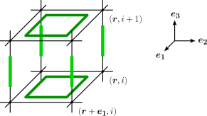
Figure 1: Lattice connectivity of the classical $D=3$ XM model.

The final form of $\mathcal{Z}^{D}$ in terms of its EDFs depends critically on the choice of basis $\psi$ in Eq. (5). As an extreme example, if $\{|\psi_{j}\rangle\}=\{\mathcal{U}_{{\sf d}}|\phi_{i}\rangle\}$, then Eq. (6) is reduced to a trivial identity with $A=1$. The choice of basis also determines whether a bond-algebraic duality is D-non-Abelian or D-Abelian, that is, whether or not it introduces local constraints when the trace is expanded. Local constraints appear if the combination of TMs between resolutions of the identity have entries that are zero with respect to the basis. Thus, given a bond-algebraic duality, it is natural to seek a basis where the relevant TMs are full, so that the duality is D-Abelian. In general, the entries of the matrices also need to be positive and expressible as products of local Boltzmann weights. Although such bases are known to exist for a large class of duality problems including TDs, we do not have general strategies for finding them.

We illustrate these ideas with a D-Abelian and a D-non-Abelian duality for the Xu-Moore (XM) model of $p+ip$ superconducting arrays Xu and Moore (2004, 2005). The model’s $D=3$ dimensional classical PF is given by (see Fig. 1)

$$\mathcal{Z}_{\sf XM}=\sum_{\{\sigma_{({\bm{r}},i)}\}}e^{\sum_{i}\sum_{\bm{r}}[K_{l}\sigma_{({\bm{r}},i)}\sigma_{({\bm{r}},i+1)}+K_{p}\square\sigma_{({\bm{r}},i)}]},$$ (7)

where $\sigma_{({\bm{r}},i)}=\pm 1$ are classical Ising variables placed at the sites $({\bm{r}},i)$ ($i$ an integer) of a cubic lattice, and $\square\sigma_{({\bm{r}},i)}\equiv\sigma_{({\bm{r}},i)}\sigma_{({\bm{r}}+{\bm{e_{2}}},i)}\sigma_{({\bm{r}}+{\bm{e_{1}}},i)}\sigma_{({\bm{r}}+{\bm{e_{1}}}+{\bm{e_{2}}},i)}$. The XM model is a $G$-model with $G=\mathds{Z}_{2}$. The TD transformation maps the model to itself with a characteristic interchange of strong and weak coupling constants Xu and Moore (2004). To recast it as a D-Abelian bond-algebraic duality, we construct plane-to-plane TMs

$$T_{1}=\prod_{\bm{r}}e^{h\sigma^{x}_{\bm{r}}},\ \ \ \ T_{0}=\prod_{\bm{r}}e^{K_{p}\square\sigma^{z}_{\bm{r}}},$$ (8)

with $\sigma^{x,z}_{\bm{r}}$ Pauli matrices acting on quantum spins at sites ${\bm{r}}$ of a ($d=2$) square lattice, $h=-\ln\tanh(K_{l})/2$, and $\square\sigma^{z}_{\bm{r}}=\sigma^{z}_{\bm{r}}\sigma^{z}_{{\bm{r}}+{\bm{e_{2}}}}\sigma^{z}_{{\bm{r}}+{\bm{e_{1}}}}\sigma^{z}_{{\bm{r}}+{\bm{e_{1}}}+{\bm{e_{2}}}}$ (see Fig. 2). To recover $\mathcal{Z}_{\sf XM}$, the trace ${{\sf Tr}}_{\phi}[(T_{1}T_{0})^{N}]$ is computed with respect to the basis $\phi$ that diagonalizes the $\sigma^{z}_{\bm{r}}$.

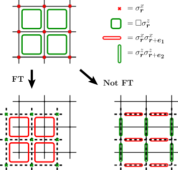
Figure 2: The quantum XM model (shown on top) is self-dual as indicated by the arrow on the left, and it is dual to the planar orbital compass model, as indicated by the arrow on the right. Direct and dual lattices are indicated with solid and dashed lines, respectively.

The TMs can be expressed as products of $t_{1,{\bm{r}}}=\cosh(h)+\sinh(h)\sigma^{x}_{\bm{r}},t_{0,{\bm{r}}}=\cosh(K_{p})+\sinh(K_{p})\square\sigma^{z}_{\bm{r}}$. We therefore let the bonds be $\{\sigma^{x}_{\bm{r}},\square\sigma^{z}_{\bm{r}}\}$. They satisfy a bond-algebraic duality induced by

$$\sigma^{x}_{\bm{r}}\mapsto\square\sigma^{x}_{\bm{r}},\ \ \ \ \square\sigma^{z}_{\bm{r}}\mapsto\sigma^{z}_{{\bm{r}}+{\bm{e_{1}}}+{\bm{e_{2}}}},$$ (9)

and illustrated in Fig. 2. The dual TMs

$$T_{1}^{D}=\prod_{\bm{r}}e^{h\square\sigma^{x}_{\bm{r}}},\ \ \ \ T_{0}^{D}=\prod_{\bm{r}}e^{K_{p}\sigma^{z}_{\bm{r}}},$$ (10)

are related to $T_{1},T_{0}$ by a unitary mapping. If we expand $\mathcal{Z}^{D}_{\sf XM}={{\sf Tr}}_{\phi}[(T_{1}^{D}T_{0}^{D})^{N}]$ with respect to $\phi$, we find that $\mathcal{Z}^{D}_{\sf XM}$ contains local constraints, so that the mapping of Eq. (9) is D-non-Abelian relative to $\phi$. It is, however, $D$-Abelian in the basis $\psi$ that diagonalizes the $\sigma^{x}_{\bm{r}}$, with respect to which we recover the traditional self-duality of the XM model Xu and Moore (2004); Cobanera et al. (2010). In the bond-algebraic approach to dualities, the role of the FT is encoded in the change of basis $\phi\mapsto\psi$ realized by a direct product of Hadamard operators $H$ satisfying $H\sigma^{z}H=\sigma^{x}$.

The bond algebra of the XM model has another local representation Nussinov and Fradkin (2005); Cobanera et al. (2010, 2011),

$$\sigma^{x}_{\bm{r}}\mapsto\sigma^{z}_{\bm{r}}\sigma^{z}_{{\bm{r}}+{\bm{e_{2}}}},\ \ \ \ \square\sigma^{z}_{\bm{r}}\mapsto\sigma^{x}_{{\bm{r}}+{\bm{e_{2}}}}\sigma^{x}_{{\bm{r}}+{\bm{e_{1}}}+{\bm{e_{2}}}}.$$ (11)

The corresponding dual TMs

$${\tilde{T}_{1}^{D}}=\prod_{\bm{r}}e^{h\sigma^{z}_{\bm{r}}\sigma^{z}_{{\bm{r}}+{\bm{e_{2}}}}},\ \ \ \ {\tilde{T}_{0}^{D}}=\prod_{\bm{r}}e^{K_{p}\sigma^{x}_{\bm{r}}\sigma^{x}_{{\bm{r}}+{\bm{e_{1}}}}},$$ (12)

yield an alternative dual partition function ${\tilde{\mathcal{Z}}^{D}_{\sf XM}}={{\sf Tr}}_{\phi}[({\tilde{T}_{1}^{D}}{\tilde{T}_{0}^{D}})^{N}]$. With $\phi$ the basis that diagonalizes the $\sigma^{z}_{\bm{r}}$, we obtain a PF with local, four-spin constraints. Relative to this basis the duality of Eq. (11) is D-non-Abelian. It is an open problem whether there is a choice of basis for which ${\tilde{\mathcal{Z}}^{D}_{\sf XM}}$ is an unconstrained canonical ensemble making the duality D-Abelian. An alternative may be to remove these constraints by reinterpreting them as gauge symmetries.

It is important to recall at this point that a TD maps a $G$-model on a lattice $\Lambda$ to an essentially unique dual model supported on the dual lattice $\Lambda^{*}$ Drühl and Wagner (1982), and the XM model is self-dual under such TDs. In contrast, the bond-algebraic duality of Eq. (11) results in a model with a Hamiltonian that differs from that of the XM model. We conclude that this bond-algebraic duality is not a TD.

Non-Abelian dualities.— Next, we show that bond-algebraic dualities exist for $G$-models with non-Abelian $G$ and no TDs. For example, consider the Euclidean lattice version Wilson (1974) of the $SU(2)$ principal chiral field Polyakov and Wiegmann (1983). This model involves an $SU(2)$-valued field $u(x)=\begin{pmatrix}u^{1}_{\ \,1}&u^{1}_{\ \,2}\\ u^{2}_{\ \,1}&u^{2}_{\ \,2}\end{pmatrix}\in SU(2)$ with action

$$S_{\sf PCh}=\frac{1}{2\lambda_{0}}\int dtdx\ {{\sf tr}}(\partial_{0}u^{*}.\partial_{0}u-\partial_{1}u^{*}.\partial_{1}u)\ .$$ (13)

The lower dot denotes matrix multiplication, $u^{*}(x)$ is the Hermitian-conjugate field, and ${{\sf tr}}$ is the $2\times 2$-matrix trace. Since $u^{*}(x)u(x)=\mathds{1}$, the lattice Euclidean path integral reduces to

$$\mathcal{Z}_{\sf PCh}=\int_{\{u_{\bm{r}}\}}e^{\frac{1}{2\lambda_{0}}\sum_{{\bm{r}}}{\sf Re}\{{{\sf tr}}(u^{*}_{{\bm{r}}+{\bm{e_{1}}}}u_{\bm{r}})+{{\sf tr}}(u^{*}_{{\bm{r}}+{\bm{e_{2}}}}u_{\bm{r}})\}}$$ (14)

on the square lattice with $SU(2)$ as the EDFs’ configuration space. Note that if we replace $SU(2)$ by $U(1)$ we obtain the $XY$-model, for which there is a $D$-Abelian duality to the solid-on-solid model Savit (1980); Cobanera et al. (2011).

To express $\mathcal{Z}_{\sf PCh}$ in terms of row-to-row transfer operators. we use covariant pairs of standard representations of $SU(2)$ and the continuous functions $C_{0}(SU(2))$ on $SU(2)$, both acting on wavefunctions on $SU(2)$. A generating set for $C_{0}(SU(2))$ is given by $(U)^{\mu}_{\ \,\nu}$ ($\mu,\nu=1,2$), where $(U)^{\mu}_{\ \,\nu}(u)=u^{\mu}_{\ \,\nu}$. Thus $U$ is a matrix-valued function. The standard representation of $SU(2)$ has infinitesimal generators $J=(J_{x},J_{y},J_{z})$ for multiplication on the right. If we write $u=e^{-{\sf i}\theta\hat{n}\cdot\vec{\sigma}/2}$, $\theta$ a finite angle, and $\hat{n}$ a unit vector, then $e^{{\sf i}\theta\hat{n}\cdot J}|v\rangle=|v.u\rangle$ for the formal basis of wavefunctions $|v\rangle$. The row-to-row transfer operators are given by

$$T_{0} = \prod_{i}e^{\frac{1}{2\lambda_{0}}{\sf Re}\{{{\sf tr}}(U^{*}_{i}.U_{i+1})\}},$$ (15)

$$T_{1} = \prod_{i}\int du\ e^{h{\sf Re}\{{{\sf tr}}(u)\}}e^{{\sf i}\theta\hat{n}\cdot J_{i}},\ \ u=e^{-{\sf i}\theta\hat{n}\cdot\vec{\sigma}/2},$$ (16)

for a parameter $h$ dependent on $\lambda_{0}$. The products are over the EDFs in a row. To recover Eq. (14), the trace ${{\sf Tr}}_{\phi}[(T_{1}T_{0})^{N}]$ is expanded with respect to the basis $|v\rangle$.

To define a bond-algebraic duality, we use the generators $j_{i}$ of left multiplication, which satisfy $e^{{\sf i}\theta\hat{n}\cdot j_{i}}|u_{i}\rangle=|u.u_{i}\rangle.$ These generators can be related to actions defined by $J$ and $U$ by the identity Susskind (1975) $j_{ia}\equiv\sum_{b=x,y,z}{{\sf tr}}(U_{i}^{*}\sigma^{a}U_{i}\sigma^{b})J_{ib}/2$, such that $[j_{i},J_{j}]=0$. The bond algebra generated by the local bonds $J_{i}$ and $U_{i}^{*}.U_{i+1}$ can be transformed to local bonds according to

$$J_{i}\mapsto-j_{i}+J_{i-1},\ \ \ U_{i}^{*}.U_{i+1}\mapsto U_{i}.$$ (17)

Proving that the mapping is induced by a unitary operator requires adding boundary terms to complete the algebra, checking that the images of the EDFs’ operators are generated by corresponding covariant pairs of representations and applying the Stone-von Neumann-Mackey theorem Rosenberg (2004) (see the Supplemental Material). It follows that

$$T_{0}^{D} = \prod_{i}\ e^{\lambda_{1}{\sf Re}\{{{\sf tr}}(U_{i})\}}\ ,$$ (18)

$$T_{1}^{D} = \prod_{i}\int du\ e^{\lambda_{2}{\sf Re}\{{{\sf tr}}(u)\}}e^{{\sf i}\theta\hat{n}\cdot(-j_{i}+J_{i-1})}$$ (19)

are unitarily equivalent to the corresponding TMs $T_{0}$ and $T_{1}$. Note that the dual variables $\hat{J}_{i},\hat{U}_{i}$

$$\hat{J}_{i}=-j_{i}+J_{i-1},\ \ \ \ \hat{U}_{i}=\cdots.U_{i+2}^{*}.U^{*}_{i+1}.U_{i}^{*}$$ (20)

that are the unitary images of the EDF operators under the duality are, as expected on general grounds, non-local collective modes. The string defining $\hat{U}_{i}$ extends to the boundary of the system, and its specific form is determined by the chosen boundary conditions.

To obtain a dual PF, we expand the trace with respect to the basis $|v_{i}\rangle$ for each $i$. The PF $\mathcal{Z}_{\sf PCh}^{D}={{\sf Tr}}_{\psi}[(T_{1}^{D}T_{0}^{D})^{N}]$ is then given by (${\bm{r}}=i{\bm{e_{1}}}+j{\bm{e_{2}}}$)

$$\int_{\{u_{\bm{r}}\}}e^{\sum_{i,j}\frac{1}{2\lambda_{0}}{\sf Re}\{{{\sf tr}}(u_{i,j}^{*}.u_{i,j+1})+{{\sf tr}}(u_{i,2j})\}}\!\!\prod_{i+j={\sf even}}\!\!\!\delta(\mathds{1},\square u_{i,j}),$$

where $\square u_{i,j}=u_{i,j}^{*}u_{i,j+1}u_{i+1,j+1}u_{i+1,j}^{*}$ (see the Supplemental Material). As for $\mathcal{Z}^{D}_{\sf XM}$, we obtain a PF with local constraints on a checkerboard. We do not know whether there is a choice of basis that removes such constraints.

We have discussed dualities for classical models, which also apply to Euclidean path-integral representations of quantum problems. This is the context in which the problem of non-Abelian dualities is typically stated. However, as explained in detail in Ref. Cobanera et al. (2011), bond-algebraic dualities provide a unified approach to classical and quantum dualities, so we can use essentially the same techniques to obtain dualities for any quantum mechanical model. The bond algebra of a quantum Hamiltonian $H=\sum_{\Gamma}h_{\Gamma}$ is the algebra generated by the local or quasi-local bonds $h_{\Gamma}$, and a bond-algebraic quantum duality is given by a mapping $h_{\Gamma}\mapsto h_{\Gamma}^{D}$ to an algebraically equivalent dual set of local or quasi-local bonds. As before, one can typically show that the isomorphism is induced by a unitary transformation, in which case $H^{D}=\sum_{\Gamma}h_{\Gamma}^{D}$ is unitarily equivalent to $H$. Take, for example, the $d=1$, infinite chain, $SU(2)$ equivalent of the $\mathds{Z}_{2}$ transverse-field Ising Hamiltonian

$$H_{\sf PCh}=\sum_{i}[\frac{1}{2}J_{i}^{2}+\frac{\lambda}{2}({{\sf tr}}(U_{i}^{*}.U_{i+1})+{{\sf tr}}(U_{i+1}^{*}.U_{i}))],$$ (21)

which is not self-dual, but has a duality to

$$H_{\sf PCh}^{D}=\sum_{i}[\frac{1}{2}(-j_{i}+J_{i-1})^{2}+\frac{\lambda}{2}({{\sf tr}}(U_{i}^{*})+{{\sf tr}}(U_{i}))],$$ (22)

as follows from Eq. (17) (see the Supplemental Material). Quantum dualities are remarkably simpler than classical dualities. They do not depend on a choice of basis, and so the distinction between D-Abelian and D-non-Abelian becomes irrelevant.

I Supplemental Material to The non-Abelian Duality Problem

We present mathematical details and clarify technical issues of results reported in the accompanying paper The non-Abelian Duality Problem.

II The Ising Model Revisited

In this section we explain how to choose the basis for expanding the traces when determining partition functions from products of transfer matrices. We illustrate the main concepts by example and use the two-dimensional Ising model Nishimori and Ortiz (2010) to show that bond-algebraic dualities may display both D-Abelian and D-non-Abelian features. The partition function of the Ising model is given by (${\bm{r}}=i{\bm{e_{1}}}+j{\bm{e_{2}}}$)

$$\mathcal{Z}_{\sf I}[K_{1},K_{2}]=\sum_{\{\sigma_{{\bm{r}}}\}}\exp[\sum_{i,j}(K_{1}\sigma_{i,j}\sigma_{i+1,j}+K_{2}\sigma_{i,j}\sigma_{i,j+1})],$$ (23)

and can be expressed as $\mathcal{Z}_{\sf I}[K_{1},K_{2}]={{\sf Tr}}_{\phi}[(T_{1}T_{0})^{N}]$ in terms of the transfer matrices

$$T_{0}=\prod_{i}\ e^{K_{1}\sigma^{z}_{i}\sigma^{z}_{i+1}},\ \ \ \ \ \ T_{1}=\prod_{i}\ (e^{K_{2}}+e^{-K_{2}}\sigma^{x}_{i}),$$ (24)

provided the trace is expanded in the basis $\phi=\{|\phi_{k}\rangle\}$ that diagonalizes the Pauli matrices $\sigma^{z}_{i}$.

The mapping

$$\sigma^{z}_{i}\sigma^{z}_{i+1}\mapsto\sigma^{z}_{i},\ \ \ \ \ \ \sigma^{x}_{i}\mapsto\sigma^{x}_{i-1}\sigma^{x}_{i},$$ (25)

illustrated in Fig. 3 defines an isomorphism of bond algebras that is induced by a unitary mapping. Thus $T_{0},T_{1}$ are dual and unitarily equivalent to

$$T_{0}^{D}=\prod_{i}\ e^{K_{1}\sigma^{z}_{i}},\ \ \ \ \ \ T_{1}^{D}=\prod_{i}\ (e^{K_{2}}+e^{-K_{2}}\sigma^{x}_{i}\sigma^{x}_{i+1}).$$ (26)

Figure 3: Duality isomorphism of bond algebras associated with the transfer matrices of the Ising model.

To compute a partition function from the dual transfer matrices via the expression $\mathcal{Z}_{\sf I}^{D}={{\sf Tr}}_{\psi}[(T_{1}^{D}T_{0}^{D})^{N}$], we need to specify a basis $\psi=\{|\psi_{k}\rangle\}$. The expansion of the trace obtained by inserting resolutions of the identity with respect to this basis must be recognizable as the partition function of a local system. In particular, the coefficients of the expansion must be non-negative, so that they can be written as Boltzman weights, and they must be products of local terms consistent with the expansion. For example, set $\psi=\phi$, the basis of the previous paragraph. Then, as will become clear below, it is convenient to split ${T}_{1}^{D}={T}_{1o}^{D}{T}_{1e}^{D}$, where

$${T}_{1o}^{D} = \prod_{i_{o}}(e^{K_{2}}+e^{-K_{2}}\sigma^{x}_{i_{o}}\sigma^{x}_{i_{o}+1}),$$ (27)

$${T}_{1e}^{D} = \prod_{i_{e}}(e^{K_{2}}+e^{-K_{2}}\sigma^{x}_{i_{e}}\sigma^{x}_{i_{e}+1}),$$ (28)

with $i_{o}=2i+1$, $i_{e}=2i$, $i\in\mathds{Z}$. We can label the members of the basis $|\phi_{k}\rangle$ in terms of strings $\sigma$ of Ising variables $\pm 1$ at sites $i$ so that $\sigma^{z}_{i}|\sigma\rangle=\sigma_{i}|\sigma\rangle\ .$ With these labels, the basis members are written as $|\sigma\rangle$. We now compute $\mathcal{Z}_{\sf I}^{D}={{\sf Tr}}_{\phi}[({T}_{1o}^{D}{T}_{1e}^{D}T_{0}^{D})^{N}]$ by expanding the trace as

$${{\sf Tr}}_{\phi}[({T}_{1o}^{D}{T}_{1e}^{D}T_{0})^{N}] =$$

$$\!\!\!\!\!\!\!\!\!\!\!\!\!\!\!\!\!\!\!\!\!\!\!\!\!\sum_{\{\sigma_{1}\},\cdots,\{\sigma_{2N}\}}\!\!\!\!\!\!\langle\sigma_{1}|{T}_{1o}^{D}|\sigma_{2}\rangle\langle\sigma_{2}|{T}_{1e}^{D}T_{0}^{D}|\sigma_{3}\rangle\cdots$$

$$\cdots \langle\sigma_{2N-1}|{T}_{1o}^{D}|\sigma_{2N}\rangle\langle\sigma_{2N}|{T}_{1e}^{D}T_{0}^{D}|\sigma_{1}\rangle,$$

where $\{\sigma_{j}\},j=1,\cdots,2N$, describes the state of row $j$. Note that $T_{0}^{D}$ is diagonal in the chosen basis. Further,

$$\langle\sigma_{j}|{T}_{1o}^{D}|\sigma_{j+1}\rangle=$$

$$\prod_{i_{o}}\langle\sigma_{i_{o},j}\sigma_{i_{o}+1,j}|e^{K_{2}}+e^{-K_{2}}\sigma^{x}_{i_{o}}\sigma^{x}_{i_{o}+1}|\sigma_{i_{o},j+1}\sigma_{i_{o}+1,j+1}\rangle,$$

and a similar factorization holds for $\langle\sigma_{j}|{T}_{1e}^{D}|\sigma_{j+1}\rangle$. The splitting ${T}_{1}^{D}={T}_{1o}^{D}{T}_{1e}^{D}$ was introduced to ensure this factorization. We can evaluate Eq. (II) by applying shifted forms of the identity

$$\langle\sigma_{1}^{\prime}\sigma_{2}^{\prime}|e^{K_{2}}+e^{-K_{2}}\sigma^{x}_{1}\sigma^{x}_{2}|\sigma_{1}\sigma_{2}\rangle=$$ (31)

$$= e^{\frac{K_{2}}{2}(\sigma_{1}^{\prime}\sigma_{1}+\sigma_{2}^{\prime}\sigma_{2})}\delta(\sigma_{1}^{\prime}\sigma_{1},\sigma_{2}^{\prime}\sigma_{2}).$$

It follows that

$${\mathcal{Z}}_{\sf I}^{D} = \sum_{\{\sigma_{{\bm{r}}}\}}\left(\prod_{i+j={\sf even}}\delta(\sigma_{i,j}\sigma_{i,j+1},\sigma_{i+1,j}\sigma_{i+1,j+1})\right)$$ (32)

$$\times\exp\Big{[}\sum_{i,j}\big{(}\frac{K_{2}}{2}\sigma_{i,j}\sigma_{i,j+1}+K_{1}\sigma_{i,2j+1}\big{)}\Big{]}.$$

The interactions in ${\mathcal{Z}}_{\sf I}^{D}$ are illustrated in Fig. 4.

Figure 4: Interactions and constraints in the dual partition function ${\mathcal{Z}}_{\sf I}^{D}$. The crosses highlight the sites where the classical Ising variables couple to a inhomogeneous external field of magnitude $K_{1}$. The heavy vertical lines indicates a nearest-neighbor Ising interaction of magnitude $K_{2}/2$. The staggered distribution of plaquettes with round corners indicates the distribution of four-spin delta constraints.

The last factor in Eq. (32) for ${\mathcal{Z}}_{\sf I}^{D}$ can be identified as a Boltzmann weight for a physical system with local interactions, one of the requirements for a good choice of basis to expand the trace in. However, the expression for the partition function in Eq. (32) also introduces local (delta function) constraints to account for the fact that the dual Boltzmann weights vanish for some configurations. It is preferable to find a basis $\psi$ where all the Boltzmann weights are strictly positive so that there are no constraints. For the Ising model, one can find such a basis by inspection. Let $\psi$ be the basis that diagonalizes the Pauli matrices $\sigma^{x}_{i}$. Then one can check that

$$\mathcal{Z}_{\sf I}[K_{1},K_{2}] = {{\sf Tr}}_{\phi}[(T_{1}T_{0})^{N}]$$ (33)

$$= {{\sf Tr}}_{\psi}[(T_{1}^{D}T_{0}^{D})^{N}]=A\mathcal{Z}_{\sf I}[K_{1}^{*},K_{2}^{*}]$$

with $\sinh(2K_{1}^{*})\sinh(2K_{2})=1=\sinh(2K_{2}^{*})\sinh(2K_{1})$. The proportionality factor $A$ is an analytic function of the couplings and size of the system Cobanera et al. (2011). We then recover the Kramers-Wannier self-duality of the Ising model.

The duality of the Ising model expressed by Eq. (32) is not a self-duality. The Kramers-Wannier self-duality as derived above is the result of combining the bond-algebraic mapping of Eq. (25) with a suitable choice of basis $\psi$. The dual partition function according to Eq. (32) has restructured the interactions drastically, but has left the couplings $K_{1},K_{2}$ essentially unchanged. Nevertheless, such dualities reveal key properties of traditional dualities. For example, consider the two-point correlator $\langle\sigma_{m^{\prime},n^{\prime}}\ \sigma_{m,n}\rangle$. In the limit in which $(m^{\prime},n^{\prime})$ is infinitely far from $(m,n)$, this correlator defines the square of the order parameter. We can compute the correlator in the dual model of Eq. (32) as

$$\langle\sigma_{m^{\prime},n^{\prime}}\ \sigma_{m,n}\rangle=$$

$$= \frac{{{\sf Tr}}_{\phi}[T^{(N-n^{\prime})}\ \sigma^{z}_{m^{\prime}}\ T^{(n^{\prime}-n)}\ \sigma^{z}_{m}\ T^{n}]}{{{\sf Tr}}_{\phi}[T^{N}]}$$

$$= \frac{{{\sf Tr}}_{\phi}[(T^{D})^{(N-n^{\prime})}\ \mu^{z}_{m^{\prime}}\ (T^{D})^{(n^{\prime}-n)}\ \mu^{z}_{m}\ (T^{D})^{n}]}{{{\sf Tr}}_{\phi}[(T^{D})^{N}]}$$

$$= \langle\mu_{m^{\prime},n^{\prime}}\ \mu_{m,n}\rangle,$$

where $T=T_{1}T_{0}$, $\ {T}^{D}={T}_{1}^{D}{T}^{D}_{0}$ (see Eq. (27)), and $\sigma^{z}\mapsto\mu^{z}_{m}=\sigma^{z}_{m}\sigma^{z}_{m+1}\sigma^{z}_{m+2}\cdots,$ the dual Pauli spin operator from Eq. (25). Hence

$$\mu_{m,n}=\sigma_{m,n}\sigma_{m+1,n}\sigma_{m+2,n}\cdots\ .$$ (35)

In the dual model ${\mathcal{Z}}_{\sf I}^{D}$, the string correlator $\langle\mu_{m^{\prime},n^{\prime}}\ \mu_{m,n}\rangle$ is (in the limit of infinite separation) the square of the order parameter. Thus, for example, if $K<K_{c}$, $\mathcal{Z}_{\sf I}$ is in its ferromagnetic phase, corresponding by duality to a phase of ${\mathcal{Z}}_{\sf I}^{D}$ dominated by strong correlations of string collective modes.

III Duality of the $SU(2)$ Principal Chiral field: Hamiltonian Formulation

This section discusses a duality for the finite system

$$H_{\sf PCh}=\frac{1}{2}\sum_{m=1}^{N}J_{m}^{2}+\frac{\lambda}{2}\sum_{m=1}^{N-1}{\sf Re}\,{{\sf tr}}(U_{m+1}^{*}.U_{m}).$$ (36)

The Hamiltonian $H_{\sf PCh}$ can be obtained as the time-continuum limit Fradkin and Susskind (1978); Kogut (1979) of the partition function of Eq. ($14$) of the accompanying paper.

III.1 Algebra of a Single Quantum Rigid Rotator

The kinematical algebra of a rigid rotator Susskind (1975) is defined by the relations among the canonical variables $J_{a},a=x,y,z$, $U^{\mu}_{\ \ \nu},\mu,\nu=1,2$,

$${}J_{a}^{\dagger} = J_{a},$$ (37)

$${}[J_{a},J_{b}] = i\epsilon_{abc}J_{c},$$ (38)

$${}[J,U] = \frac{1}{2}U.\sigma,$$ (39)

$${}U^{*}.U = U.U^{*}=\mathds{1},$$ (40)

introduced in the accompanying paper. Here $\sigma$ denotes a standard Pauli matrix. The low dot denotes matrix multiplication to distinguish it from tensor multiplication, and a centered dot denotes the standard Euclidean inner product. For example, $J\cdot J=J_{x}^{2}+J_{y}^{2}+J_{z}^{2}$, and

$$[J,U]=\frac{1}{2}U.\sigma\ \leftrightarrow\ [J_{a},U^{\mu}_{\ \ \nu}]=\frac{1}{2}\sum_{\kappa}U^{\mu}_{\ \ \kappa}\sigma^{\kappa}_{a\ \nu}\ .$$ (41)

Eqs. (37) and (40) imply ${}[J,U^{*}]=-\sigma.U^{*}/2.$

The algebra above affords a set of position-like operators $U,U^{*}$ and conjugate momenta $J_{a}$ that suffice to specify completely the kinematics of quantum tops. It is useful however to introduce three additional operators

$$j_{a}\equiv\frac{1}{2}\sum_{b}{{\sf tr}}(U^{*}.\sigma_{a}.U.\sigma_{b})J_{b},\qquad a=x,y,z$$ (42)

or just $j={{\sf tr}}(U^{*}.\sigma.U.(\sigma\cdot J))/2$ for short, having some very useful properties:

$${}j_{a}^{\dagger} = j_{a},$$ (43)

$${}[j_{a},j_{b}] = -i\epsilon_{abc}j_{c},$$ (44)

$${}[j,U] = \frac{1}{2}\sigma.U,$$ (45)

$${}[j_{a},J_{b}] = 0,$$ (46)

$${}j\cdot j = J\cdot J.$$ (47)

Direct proofs of these relations, based on definition Eq. (42) and relations (37), (38), (39), (40), can be found in Sect. III.3 of this Supplemental Material. Notice that Eqs. (43) and (45) imply that ${}[j,U^{*}]=-{U^{*}}.\sigma/2.$

III.2 Bond-algebraic Duality Transformation

This section describes the construction of a dual representation of the Hamiltonian $H_{\sf PCh}$ of Eq. (36). The starting point is the selection of a suitable set of bonds as generators of the bond algebra of interactions. One convenient choice is

$$J_{m},\qquad m = 1,\cdots,N$$ (48)

$$U_{m+1}^{*}.U_{m},\ U_{m}^{*}.U_{m+1},\qquad m = 1,\cdots,N-1,$$ (49)

We call the algebra they generate $\mathcal{A}_{\sf PCh}$. Notice that $H_{\sf PCh}\in\mathcal{A}_{\sf PCh}$, but the bond algebra does not include the position-like operators $U_{m},U_{m}^{*},\ m=1,\cdots,N$. It will be useful later to change this by adding a boundary term

$$U_{N},\qquad U_{N}^{*},$$ (50)

to the list of generators of $\mathcal{A}_{\sf PCh}$. The resulting extended algebra, still denoted by $\mathcal{A}_{\sf PCh}$, does include the $U_{m},U_{m}^{*},\ m=1,\cdots,N$, since

$$U_{m} = U_{N}.(U_{N}^{*}.U_{N-1}).\cdots.(U_{m+1}^{*}.U_{m}),$$ (51)

$$U_{m}^{*} = (U_{m}^{*}.U_{m+1}).\cdots.(U_{N-1}^{*}.U_{N}).U_{N}^{*}\ .$$ (52)

The extended algebra $\mathcal{A}_{\sf PCh}$ is simply a direct product of $N$ copies of the algebra generated by a single rigid rotator $J,U,U^{*}$. However, what is required is an understanding of the structure of $\mathcal{A}_{\sf PCh}$ from the point of view of the local interaction terms in $H_{\sf PCh}$. The relations (other than commutation) between the bond generators of Eqs. (48), (49), and (50) are $U_{N}^{*}.U_{N}=\mathds{1}$, $(U_{m+1}^{*}.U_{m}).(U_{m}^{*}.U_{m+1})=\mathds{1}$, $[J_{m,a},\ J_{n,b}]=i\epsilon_{abc}J_{m,c}\,\delta_{m,n}$ for $m=2,\cdots,N-1$,

$${}[J_{m},U_{m}^{*}.U_{m+1}]=-\frac{1}{2}\sigma.U_{m}^{*}.U_{m+1},$$ (53)

$${}[J_{m},U_{m-1}^{*}.U_{m}]=\frac{1}{2}U_{m-1}^{*}.U_{m}.\sigma\ ,$$ (54)

and at the boundaries, $[J_{1},U_{1}^{*}.U_{2}]=-\frac{1}{2}\sigma.U_{1}^{*}.U_{2}$, $[J_{N},U_{N-1}^{*}.U_{N}]=\frac{1}{2}U_{N-1}^{*}.U_{N}.\sigma$, and $[J_{N},U_{N}^{*}]=-\frac{1}{2}\sigma.U_{N}^{*}$. Relations that follow by Hermitian conjugation from those listed have been omitted.

The goal is to construct a mapping that preserves these algebraic relations and locality. For instance (see Fig. 5),

$$U_{N}^{*} \mapsto U_{N},\qquad U_{m-1}^{*}.U_{m}\mapsto U_{m-1},$$ (55)

$$J_{1} \mapsto -j_{1},\qquad J_{m}\mapsto-j_{m}+J_{m-1},$$ (56)

for $m=2,\cdots,N.$

Figure 5: Duality automorphism for the quantum chain of rigid rotators, shown for three sites ($N=3$).

It is not necessary to specify the action of this mapping on the $j_{m}$, since the $j_{m}$ are functions of $J_{m},U_{m},U_{m}^{*}$ (see Eq. (42)).

As noted in the accompanying paper, to verify that the bond-algebra mapping defined above is induced by a unitary map, we can invoke the Stone-von Neumann-Mackey theorem Rosenberg (2004). In order to do so, we need to verify that the operators of the elementary degrees of freedom are transformed into operators of a covariant pair of representations as required by the theorem. We can express the images of the operators in terms of the bonds (including the boundary terms) directly. A benefit of doing so is that these images define collective modes of interest.

The dual momenta $\hat{J}_{m}$ are by definition the image $J_{m}\mapsto\hat{J}_{m}$, and are obtained directly from Eq. (56),

$$\hat{J}_{1}=-j_{1},\qquad\hat{J}_{m}=J_{m-1}-j_{m},$$ (57)

for $m=2,\cdots,N$. To compute the dual position-like operators it is necessary to exploit the decompositions of Eqs. (51) and (52). These decompositions combined with Eq. (55) yield

$$U_{m}\mapsto U_{N}^{*}.\cdots.U_{m}^{*}\equiv\hat{U}_{m},,$$ (58)

and $U_{m}^{*}\mapsto U_{m}.\cdots.U_{N}\equiv\hat{U}_{m}^{*}$. It can be checked that the dual variables $\hat{J}_{m},\hat{U}_{m},\hat{U}_{m}^{*}$ commute on different sites, and satisfy the relations of Eqs. (37), (38), (39), and (40), as required for a covariant pair of representations.

Similarly to the dual variables, the dual Hamiltonian is computed as $H_{\sf PCh}\mapsto H_{\sf PCh}^{D}$. Hence

$$\!\!\!\!\!\!\!\!\!H_{\sf PCh}^{D}=\frac{1}{2}j_{1}^{2}+\!\!\sum_{m=1}^{N-1}\Big{[}\frac{1}{2}(j_{m+1}-J_{m})^{2}+\frac{\lambda}{2}{\sf Re}\,{{\sf tr}}(U_{m})\Big{]}.$$ (59)

To gain insight into the physical meaning of Eq. (59) it is useful to discuss the global symmetries of $H_{\sf PCh}$ and their dual representation. On one hand, the interaction terms ${\sf Re}\,{{\sf tr}}({U}_{m+1}^{*}.{U}_{m})$, $m=1,\cdots,N-1$, are invariant under right and left multiplication, $U_{m}\rightarrow{U}_{m}.v$ and $U_{m}\rightarrow v.{U}_{m}$. It follows that $H_{\sf PCh}$ has a global $SU(2)\times SU(2)$ symmetry, with infinitesimal generators $J\equiv\sum_{m=1}^{N}J_{m}$ and $j\equiv\sum_{m=1}^{N}j_{m}$ that commute with $H_{\sf PCh}$. On the other hand, the dual Hamiltonian $H_{\sf PCh}$ contains the terms ${\sf Re}\,{{\sf tr}}(U_{m})$, $m=1,\cdots,N-1$, invariant only under the adjoint (anti)action, ${{\sf tr}}(v^{*}.U_{m}.v)={{\sf tr}}(U_{m}).$ It may seem that a symmetry has been lost.

The duality maps the symmetry generators $j,J$ to dual symmetry generators

$$\hat{J}=\sum_{m=1}^{N}\hat{J}_{m}=-j_{1}+\sum_{m=2}^{N}(-j_{m}+J_{m-1}),$$ (60)

$$\hat{j}=\sum_{m=1}^{N}\hat{j}_{m}=\sum_{m=1}^{N}\frac{1}{2}{{\sf tr}}(\hat{U}_{m}^{*}.\sigma.\hat{U}_{m}.(\sigma\cdot\hat{J}_{m})).$$ (61)

The Hamiltonian $H_{\sf PCh}^{D}$ commutes with $\hat{j},\hat{J}$ by construction (the duality mapping preserves all algebraic relations), meaning that no symmetry has been lost. Notice that $\hat{j}$ presents a highly non-local structure in terms of $J_{m},U_{m},U_{m}^{*}$.

III.3 Further Results on the Algebra of a Single Quantum Rigid Rotator

Next it is shown that the operators $j_{a}$ defined in Eq. (42) satisfy the relations listed in Eqs. (45) and (47). The first step is to introduce the adjoint representation of the $SU(2)$ Lie algebra via its double-covering homorphism $R$ to $SO(3)$, $U\ \mapsto\ R(U),$ defined implicitly by

$$U.\sigma_{a}.U^{*}=\sum_{b}\sigma_{b}R(U)^{b}_{\ \ a}.$$ (62)

Since ${{\sf tr}}(\sigma_{a}.\sigma_{b})/2=\delta_{ab}$, $R(U)$ reads

$$R(U)^{b}_{\ \ a}={{\sf tr}}(U.\sigma_{a}.U^{*}.\sigma_{b})/2.$$ (63)

It follows that Eq. (42) can be rewritten as $j_{a}=\sum_{b}R(U^{*})^{b}_{\ \ a}J_{b}.$

From Eq. (63),

$$[J_{a},R(U^{*})^{b}_{\ \ c}]=i\epsilon_{abd}R(U^{*})^{d}_{\ \ c}.$$ (64)

Also, $[j_{a},U]=\frac{1}{2}\sum_{b}U.\sigma_{b}R(U^{*})^{b}_{\ \ a}=\frac{1}{2}\sigma_{a}.U,$ where the last equality follows from Eq. (62) ( the conjugate relation $[j_{a},U^{*}]=-U^{*}.\sigma_{a}/2$ follows in the same way). Combining this last result with Eq. (64) gives $[j_{b},J_{a}]=i\sum_{c,d}(-\epsilon_{adc}+\epsilon_{cad})R(U^{*})^{c}_{\ \ b}J_{d}=0$, and

$$j\cdot j=\sum_{a}(\sum_{b}J_{b}R(U^{*})^{b}_{\ \ a})(\sum_{c}R(U^{*})^{c}_{\ \ a}J_{c})$$ (65)

$$+\sum_{a}(\sum_{b}[R(U^{*})^{b}_{\ \ a},J_{b}])(\sum_{c}R(U^{*})^{c}_{\ \ a}J_{c})=J\cdot J,$$

where the homomorphism property of $R$ was used to simplify $\sum_{a}R(U^{*})^{b}_{\ \ a}R(U^{*})^{c}_{\ \ a}=\delta^{b}_{\ \ c}.$

To check the commutator $[j_{a},j_{b}]$, direct computation gives

$$[j_{a},j_{b}]=-i\epsilon_{dec}R(U^{*})^{d}_{\ \ a}R(U^{*})^{e}_{\ \ b}J_{c}.$$ (66)

Since $R(U)\in SO(3)$, $\det R(U)=1$. It follows that $\epsilon_{dec}R(U^{*})^{d}_{\ \ a}R(U^{*})^{e}_{\ \ b}=\epsilon_{abf}R(U^{*})^{c}_{\ \ f}.$ Then Eq. (66) simplifies to read

$$[j_{a},j_{b}]=-i\epsilon_{abf}\sum_{c}R(U^{*})^{c}_{\ \ f}J_{c}=-i\epsilon_{abc}\ j_{c}\ .$$ (67)

It is only left to show that $j_{a}^{\dagger}=\frac{1}{2}\sum_{b}\ ([J_{b},{{\sf tr}}(U^{*}.\sigma_{a}.U.\sigma_{b})]+{{\sf tr}}(U^{*}.\sigma_{a}.U.\sigma_{b})J_{b})=j_{a}$. The commutator vanishes by virtue of Eq. (64).

References

• Kramers and Wannier (1941) H. A. Kramers and G. H. Wannier, Phys. Rev., 60, 252 (1941).
• Savit (1980) R. Savit, Rev. Mod. Phys., 52, 453 (1980).
• Drühl and Wagner (1982) K. Drühl and H. Wagner, Ann. Phys. (N.Y.), 141, 225 (1982).
• Malyshev and Petrova (1983) V. A. Malyshev and E. N. Petrova, J. of Math. Sci., 21, 877 (1983).
• Mandelstam (1979) S. Mandelstam, Phys. Rev. D, 19, 2391 (1979).
• Alvarez et al. (1994) E. Alvarez, L. A. Gaume,  and Y. Lozano, Nuc. Phys. B, 424, 155 (1994).
• Nussinov and Ortiz (2009) Z. Nussinov and G. Ortiz, Phys. Rev. B, 79, 214440 (2009).
• Cobanera et al. (2010) E. Cobanera, G. Ortiz,  and Z. Nussinov, Phys. Rev. Lett., 104, 020402 (2010).
• Cobanera et al. (2011) E. Cobanera, G. Ortiz,  and Z. Nussinov, Adv. in Phys., 60, 679 (2011).
• Wilson (1974) K. G. Wilson, Phys. Rev. D, 10, 2445 (1974).
• Kitaev (2003) A. Kitaev, Ann. of Phys., 303, 2 (2003).
• Zamolodchikov and Monastyrsky (1979) A. Zamolodchikov and M. Monastyrsky, JETP, 50, 167 (1979).
• Drouffe et al. (1979) J. Drouffe, C. Itzykson,  and J. Zuber, Nuc. Phys. B, 147, 132 (1979).
• Orland (1980) P. Orland, Nucl. Phys., B163, 275 (1980).
• Somma et al. (2007) R. D. Somma, C. D. Batista,  and G. Ortiz, Phys. Rev. Lett., 99, 030603 (2007).
• Xu and Moore (2004) C. Xu and J. E. Moore, Phys. Rev. Lett., 93, 047003 (2004).
• Xu and Moore (2005) C. Xu and J. Moore, Nuc. Phys. B, 716, 487 (2005).
• Nussinov and Fradkin (2005) Z. Nussinov and E. Fradkin, Phys. Rev. B, 71, 195120 (2005).
• Polyakov and Wiegmann (1983) A. Polyakov and P. Wiegmann, Phys. Lett. B, 131, 121 (1983).
• Susskind (1975) J. K. L. Susskind, Phys. Rev. D, 11, 395 (1975).
• Rosenberg (2004) J. Rosenberg, in Operator Algebras, Quantization and Noncommutative Geometry, A Centennial Celebration Honoring John von Neumann and Marshall H. Stone, Contemporary Mathematics, Vol. 365 (American Mathematical Society, http://www.ams.org/, 2004) pp. 331–354.

References

• Nishimori and Ortiz (2010) H. Nishimori and G. Ortiz, Elements of Phase Transitions and Critical Phenomena (Oxford University Press, 2010).
• Cobanera et al. (2011) E. Cobanera, G. Ortiz,  and Z. Nussinov, Adv. in Phys., 60, 679 (2011).
• Fradkin and Susskind (1978) E. Fradkin and L. Susskind, Phys. Rev. D, 17, 2637 (1978).
• Kogut (1979) J. B. Kogut, Rev. Mod. Phys., 51, 659 (1979).
• Susskind (1975) J. K. L. Susskind, Phys. Rev. D, 11, 395 (1975).
• Rosenberg (2004) J. Rosenberg, in Operator Algebras, Quantization and Noncommutative Geometry, A Centennial Celebration Honoring John von Neumann and Marshall H. Stone, Contemporary Mathematics, Vol. 365 (American Mathematical Society, http://www.ams.org/, 2004) pp. 331–354.