Popper’s Experiment: A Modern Perspective

Abstract

Karl Popper had proposed an experiment to test the standard interpretation of quantum mechanics. The proposal survived for many year in the midst of no clear consensus on what results it would yield. The experiment was realized by Kim and Shih in 1999, and the apparently surprising result led to lot of debate. We review Popper’s proposal and its realization in the light of current era when entanglement has been well studied, both theoretically and experimentally. We show that the “ghost-diffraction” experiment, carried out in a different context, conclusively resolves the controversy surrounding Popper’s experiment.

I Introduction

Quantum mechanics is probably the only theory which holds the unique position of being highly successful, and yet being least understood. Opinion is divided on whether it describes an underlying reality associated with physical systems or whether it is a mathematical tool to calculate the inherently probabilistic outcomes of measurement of microscopic systems. The nonlocal character of quantum mechanics, in particular, has been a source of discomfort right from the time of its inception. Einstein Podolsky and Rosen, in their seminal paper, introduced a thought experiment, which became famous as the EPR experiment, articulating the disagreement of quantum theory with the classical notion of locality epr .

Sir Karl Raimund Popper (1902-1994) is regarded as one of the greatest philosophers of science of the 20th century. Although not initially trained as a physicist, he was deeply intrigued by quantum mechanics, and its philosophical implications. He studied quantum mechanics and the various ideas associated with it deeply, to the level of finally putting up an interesting challenge to one of its interpretations. Being a realist, he believed in the reality of the state of an isolated particle. The standard interpretation of quantum mechanics, many times called the Copenhagen interpretation, proposed by Niels Bohr, assumes that certain states of two well-separated non-interacting particles can only be described as a composite whole, and disturbing one part, necessarily disturbs the other part. Einstein had called such effects as “spooky action at a distance.” Karl Popper was in disagreement with such an interpretation of quantum mechanics. He proposed an experiment, which he chose to call a variant of the EPR experiment, to test the standard interpretation of quantum theory popper ; popper1 . It later came to be known as Popper’s experiment.

II Popper’s Experiment

Popper’s proposed experiment consists of a source that can generate pairs of particles traveling to the left and to the right along the $x$-axis. The momentum along the $y$-direction of the two particles is entangled in such a way so as to conserve the initial momentum at the source, which is zero. There are two slits, one each in the paths of the two particles. Behind the slits are semicircular arrays of detectors which can detect the particles after they pass through the slits (see FIG. 1).

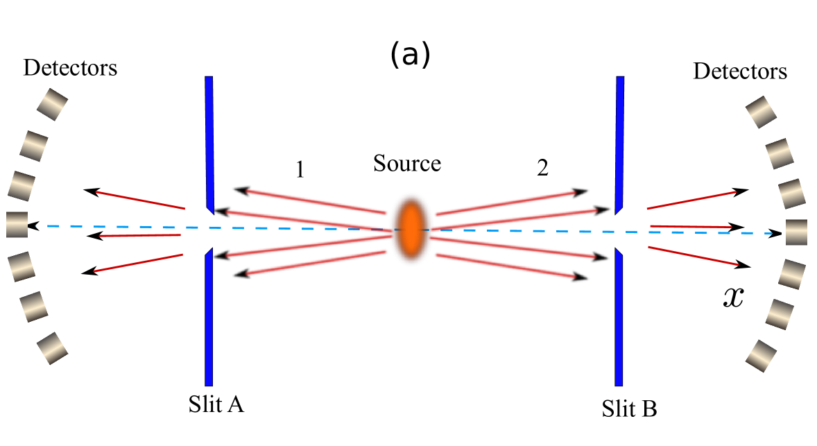
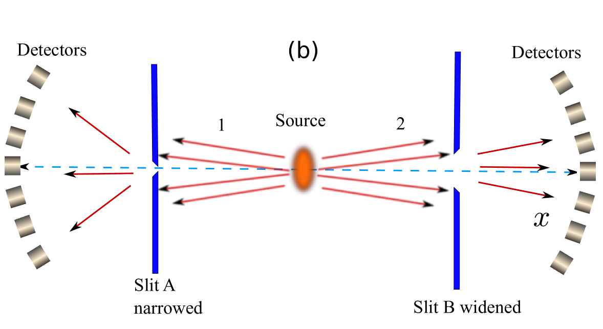
Figure 1: Schematic diagram of Popper’s thought experiment. (a) With both slits, the particles are expected to show scatter in momentum. (b) By removing slit B, Popper believed that the standard interpretation of quantum mechanics could be tested.

Being entangled in momentum space implies that in the absence of the two slits, if a particle on the left is measured to have a momentum $p$, the particle on the right will necessarily be found to have a momentum $-p$. One can imagine a state similar to the EPR state, $\psi(y_{1},y_{2})=\!\int_{-\infty}^{\infty}e^{ipy_{1}/\hbar}e^{-ipy_{2}/\hbar}dp$. As we can see, this state also implies that if a particle on the left is detected at a distance $y$ from the horizontal line, the particle on the right will necessarily be found at the same distance $y$ from the horizontal line. It appears, however, that a hidden assumption in Popper’s setup is that the initial spread in momentum of the two particles is not very large. Popper argued that because the slits localize the particles to a narrow region along the $y$-axis, they experience large uncertainties in the $y$-components of their momenta. This larger spread in the momentum will show up as particles being detected even at positions that lie outside the regions where particles would normally reach based on their initial momentum spread. This is generally understood as a diffraction spread.

Popper suggested that slit A be narrowed, and slit B be made very large. In this situation, Popper argued that when particle 1 passes through slit A, it is localized to within the width of the slit. He further argued that the standard interpretation of quantum mechanics tells us that if particle 1 is localized in a small region of space, particle 2 should become similarly localized, because of entanglement. The standard interpretation says that if one has knowledge about the position of particle 2, that should be sufficient to cause a spread in the momentum, just from the Heisenberg uncertainty principle.

Popper said that he was inclined to believe that there will be no spread in the particles at slit B, just by putting a narrow slit at A. However, Popper was open to the possibility of the other outcomes of the experiment: popper

“What would be the position if our experiment (against my personal expectation) supported the Copenhagen interpretation – that is, if the particles whose y-position has been indirectly measured at B show an increased scatter?
This could be interpreted as indicative of an action at a distance …”

Popper’s proposed experiment came under lot of attention, especially because it represented an argument which was falsifiable, an experiment which could actually be carried out sudbery ; sudbery2 ; krips ; collet ; storey ; redhead ; nha ; peres ; hunter ; sancho ; tqijqi ; popperreply ; angelidis .

III The Debate

In 1985, Sudbery pointed out that the EPR state already contained an infinite spread in momenta, tacit in the integral over $p$ in a state like $\psi(y_{1},y_{2})=\!\int_{-\infty}^{\infty}e^{ipy_{1}/\hbar}e^{-ipy_{2}/\hbar}dp$. So no further spread could be seen by localizing one particle sudbery ; sudbery2 . Sudbery further stated that collimating the original beam, so as to reduce the momentum spread, would destroy the correlations between particles 1 and 2. For some reason, the implication of Sudbery’s point was not fully understood.

Redhead theoretically analyzed a scenario where Popper’s proposed experiment is carried out using a broad source. He concluded that it could not yield the effect Popper that was seeking redhead .

Krips did an analysis of entangled particles, and predicted that in coincident counting, narrowing slit A would lead to increase in the width of the diffraction pattern behind slit B (in coincident counting) krips . He, however, did not talk about what kind of spread one should expect for particle 2, for a fixed width of slit A.

In 1987 Collet and Loudon raised an objection to Popper’s proposal collet . They pointed out that because the particle pairs originating from the source had a zero total momentum, the source could not have a sharply defined position. They argued that once the uncertainty in the position of the source is taken into account, the blurring introduced washes out the Popper effect. This objection, however, was effectively countered by Popper who argued that if the source was attached to an object of large mass, the objections of Collet and Loudon would not hold popperreply . Now it has been experimentally demonstrated that a broad Spontaneous Parametric Downconversion (SPDC) source can be set up to give a strong correlation between the photon pairs ghostimage . It has been theoretically shown that in such entangled EPR pairs, the particles can only be detected in opposite directions peres1 ; struyve .

In short, none of the objections raised against Popper’s experiment could convincingly demonstrate if there was a problem with the proposal. More surprisingly, Popper’s inference that according to Copenhagen interpretation, localizing one particle should lead to the same kind of momentum spread in the other particle, was not refuted by anybody. Thus, Popper’s proposed experiment acquired the stature of a crucial test of the standard interpretation of quantum mechanics.

IV Realization of Popper’s Experiment and the Pandemonium

The experiment was realized in 1999 by Kim and Shih using a SPDC photon source which generated entangled photons shih ; shih1 . It appears that another strong proponent of “realism” and a friend of Karl Popper, Thomas Angelidis, had convinced the authors to pursue this difficult experiment angelidis ; shih ; shih1 . Their ingenious method employed a converging lens to create a ghost image of slit A at slit B. With this they effectively overcame the objection of Collet and Loudon collet .

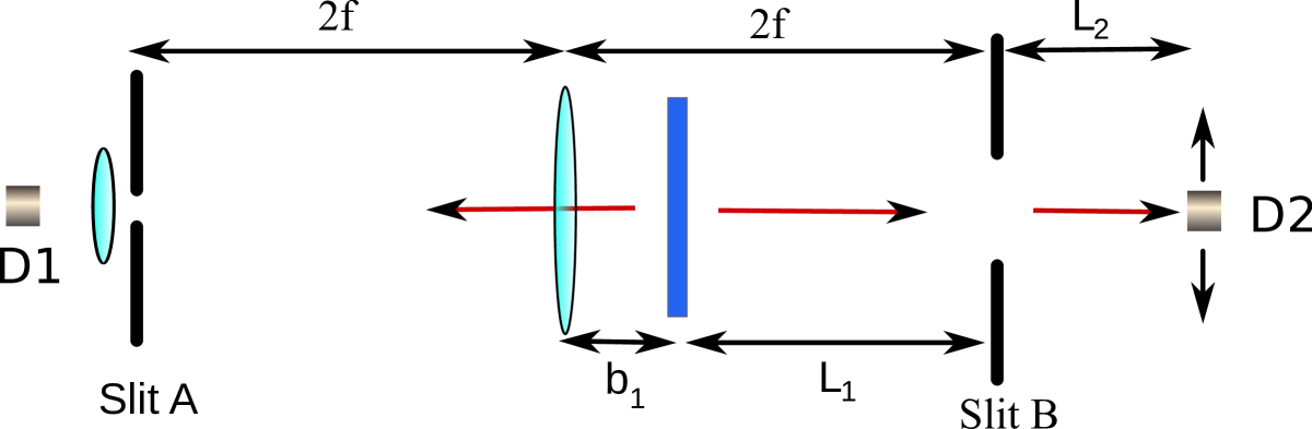
Figure 2: Setup of the photon experiment by Kim and Shih, shih aimed at realizing Popper’s proposal. Slit A is narrow while slit B is left wide open.

In their experiment, Kim and Shih did not observe an extra spread in the momentum of particle 2 due to particle 1 passing through a narrow slit. In fact, the observed momentum spread was narrower than that contained in the original beam. Taken at face value, this observation seemed to imply that Popper was right, and the Copenhagen interpretation was wrong. The experiment resulted in wild confusion over what it implied. R. Plaga used the results of Kim and Shih’s experiment to claim that an extension of Popper’s experiment can be used to test interpretations of quantum mechanics plaga . Short criticized Kim and Shih’s experiment, arguing that because of the finite size of the source, the localization of particle 2 was imperfect, short which led to a smaller momentum spread than expected. But the question still remained open as to what the result would have been had the localization of particle 2 been perfect.

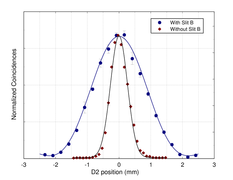
Figure 3: Results of the photon experiment by Kim and Shih, shih aimed at realizing Popper’s proposal. The diffraction pattern in the absence of slit B (diamond symbols) is much narrower than that in the presence of a real slit (round symbols).

Thomas Angelidis called the result of Kim and Shih’s experiment a “null result,” almost no momentum spread for particle 2. He argued that the experiment showed that no nonlocality exists angelidis . He further criticized Sudbery’s position that the EPR state already contained an infinite momentum spread, and argued that the experiment refuted that deduction. Angelidis had predicted that in the absence of slit B, particle 2 would go undisturbed, precisely as locality demands. He claimed that his prediction was vindicated by Kim and Shih’s experiment.

Unnikrishnan went to the extent of claiming that Kim and Shih’s experiment was proof of the absence of nonlocality in quantum mechanics unni1 ; unni2 . His argument is as follows. If there were an actual reduction of the state when the particle 1 went through slit A, particle 2 would get localized in a narrow region of space, and in the subsequent evolution, experience a greater spread in momentum. If no extra spread in the momentum of particle 2 is observed, it implies that there is no nonlocal effect of the measurement of particle 1 on particle 2. The tacit assumption here is that the correlation observed in the detected positions of particles 1 and 2, in the absence of the slits, could be explained in some other way, without invoking a nonlocal state reduction. He used it to propose his own resolution of the EPR puzzle unni2 .

V A Discrete Version of Popper’s Experiment

One difficulty with Popper’s proposed experiment and its realization is that they use continuous degrees of freedom, and it is not clear if invoking the uncertainty principle in an ad-hoc manner will lead to correct results. The essence of Popper’s argument, at least as far as nonlocality and the Copenhagen interpretation are concerned, is not based on the precise variables he chose to study, namely position and momentum. Any two variables which do not commute with each other should serve the purpose, as localizing one would lead to spread in the other. In the following, we present a discrete model which captures the essence of Popper’s proposed experiment tqijqi .

V.1 The model

Consider two spin-1 particles $A$ and $B$, emitted from a source $S$ such that $A$ travels along negative $y$ direction, and $B$ travels along positive $y$ direction. The particles start from a spin state which is entangled in such a way that if z-component of the $A$ spin is found to have value $+1$, the z-component of $B$ will necessarily have value $-1$. The initial spin state of the combined system can be written as

$$|\psi\rangle=\alpha|A_{z};+1\rangle|B_{z};-1\rangle+\beta|A_{z};0\rangle|B_{z};0\rangle+\alpha|A_{z};-1\rangle|B_{z};+1\rangle$$ (1)

where $|A_{z};m\rangle$ and $|B_{z};m\rangle$ represent the eigenstates of the z-component of the spins $A$ and $B$ respectively, with eigenvalue $m$. Also, the state $|\psi\rangle$ is normalized, so that $2\alpha^{2}+\beta^{2}=1$. Here, the z-components of the spins can be thought as playing the role of momenta in the $y$ direction of the two particles in Popper’s experiment. In that case, the x-component of the spin here can play the role of position of the two particles along $y$ axis, in Popper’s experiment. The two components of the spin do not commute with each other, so localizing one in its eigenvalues, will necessarily cause a spread in the eigenvalues of the other. Thus, this spin system is completely analogous, in spirit, to the system of entangled particles, considered by Popper.

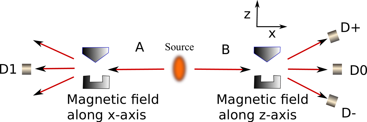
Figure 4: Schematic diagram of a discrete version of Popper’s experiment using entangled spin-1 particles. Detector $D1$ detects particle A, and particle B is detected by detectors $D+$, $D0$ and $D-$.

Next, we have to have a mechanism which is equivalent to localizing the particle 1, in Popper’s experiment, in space (what he wanted to achieve by putting a slit). To achieve an equivalent of localizing the particle 1, in Popper’s experiment, we put a Stern-Gerlach field in the path of particle $A$, pointing along the $x$ axis, but inhomogeneous along the (say) z-axis. This will split the particle $A$ into a superposition of three wave packets, spatially separated in the $z$ direction, entangled with the three spin states $|A_{x};+1\rangle$, $|A_{x};0\rangle$ and $|A_{x};-1\rangle$. Then we put a detector $D1$ in the path of this particle such that, it detects the central wave packet and localizes the x-component of spin $A$ to the state $|A_{x};0\rangle$. This achieves, what slit A was supposed to achieve in Popper’s experiment, but actually never did, namely localizing the particle in position.

On the other side of the source, we can have a Stern-Gerlach field, in the path of particle $B$, pointing along the z-direction. This will split particle $B$ into a superposition of three wave-packets, entangled with the three spin states $|B_{z};+1\rangle$, $|B_{z};0\rangle$ and $|B_{z};-1\rangle$. We have three detectors, $D+$, $D0$ and $D-$, to detect one component each of the $z$-component of spin $B$.

V.2 What do we expect?

Now, the $z$-components of spins $A$ and $B$ are entangled. So, it is indisputable that if one finds $A$ in $|A_{z};+1\rangle$ state, $B$ would be found in $|B_{z};-1\rangle$ state, and if one finds $A$ in $|A_{z};-1\rangle$ state, $B$ would be found in $|B_{z};+1\rangle$ state, and so on. Also, one can easily verify that if one measures the $x$ component of spin $A$ and finds it in the state $|A_{x};0\rangle$, one would find the $x$-component of spin $B$ in the state $|B_{x};0\rangle$. But, as operators $B_{x}$ and $B_{z}$ do not commute, if one finds spin $A$ in the state $|A_{x};0\rangle$, there should be a spread in the eigenstates of $B_{z}$. In Popper’s experiment, this would be equivalent to saying, that if particle 1 is localized in position, there should be a spread seen in the momentum of particle 2. This is what the Copenhagen interpretation predicts. At this stage, the equivalence of this experiment with Popper’s experiment is complete.

In addition, if one applies Unnikrishnan’s argumentunni1 to the present model, detecting particle $A$ in the detector $D1$ leading to observation of a spread in the counts of particle $B$ in the three detectors, amounts to a nonlocal action at a distance.

V.3 Result of the thought experiment

Let us now carry out this thought experiment and see what we get. To start with, we first remove the detector and the Stern-Gerlach field from the path of particle $A$. We start from a spin state $|\psi\rangle$ where $\beta=\sqrt{0.9}$ and $\alpha=\sqrt{0.05}$, which has the following form:

$$|\psi\rangle = \sqrt{0.05}|A_{z};+1\rangle|B_{z};-1\rangle+\sqrt{0.9}|A_{z};0\rangle|B_{z};0\rangle$$ (2)

$$+\sqrt{0.05}|A_{z};-1\rangle|B_{z};+1\rangle$$

It is trivial to see that the three detectors on the right will click in the following manner. The detector $D0$ will show 90 percent counts and the other two will have 5 percent each (see Fig. 4a).

Figure 5: Results that the detectors $D+$, $D0$ and $D-$ are expected to show (a) without the detector $D1$ and the Stern-Gerlach field in the path of particle A, and (b) with coincident counting with the detector $D1$. Here, detector positions $-1,0,+1$ correspond to the detectors $D-$, $D0$ and $D+$ respectively.

Next we put the Stern-Gerlach field and the detector in the path of particle $A$. As in Popper’s experiment, we have to do coincident count between the detector on the left, and the detectors on the right. As we are measuring the $x$-component of the spin $A$ on the left, it would be natural to write the state (2) in terms of the eigenstates $|A_{x};m\rangle$. In this form, the state $|\psi\rangle$ looks like

$$|\psi\rangle = |A_{x};+1\rangle({\sqrt{0.05}\over 2}|B_{z};+1\rangle+{\sqrt{0.9}\over\sqrt{2}}|B_{z};0\rangle$$

$$+{\sqrt{0.05}\over 2}|B_{z};-1\rangle)$$

$$-\sqrt{0.05}|A_{x};0\rangle({1\over\sqrt{2}}|B_{z};+1\rangle-{1\over\sqrt{2}}|B_{z};-1\rangle)$$

$$+|A_{x};-1\rangle({\sqrt{0.05}\over 2}|B_{z};+1\rangle-{\sqrt{0.9}\over\sqrt{2}}|B_{z};0\rangle$$

$$+{\sqrt{0.05}\over 2}|B_{z};-1\rangle)$$

It is clear from (LABEL:fstate), that in a coincident count between the detector on the left and the detectors on the right, spin $A$ is found in state $|A_{x};0\rangle$ by choice, and spin $B$ ends up in the state ${1\over\sqrt{2}}(|B_{z};+1\rangle-|B_{z};-1\rangle)$. This means that the detectors on the right will have 50 percent count each in the detectors $D+$ and $D-$, and no count in the detector $D0$! (see Fig. 4b) To start with, the z-component of spin $B$ was predominantly localized in the state $|B_{z};0\rangle$, as seen in the experiment without the detector and the field for particle $A$. Localizing the spin $A$ in the state $|A_{x};0\rangle$, results in a large scatter in the $z$-component of spin $B$. In Popper’s experiment, this will be equivalent to saying that localizing particle 1 in space, leads to a scatter in the momentum of particle 2. Thus we reach the same conclusion that Popper said, Copenhagen interpretation would lead to. But the difference here is that, looking at (LABEL:fstate) nobody would say that in actually doing this experiment, one would not see the result obtained here. This comes out just from the mathematics of quantum mechanics, without any interpretational difficulties, as in Popper’s original experiment.

In the spirit of Popper’s experiment, this discrete model really shows “spooky action at a distance”.

VI Analysis of Popper’s Proposal

One important thing that one can learn from the discrete version described above, is the following. The two peaks seen in the coincident counting in FIG. 5(b), were already present in the initial state as the two little peaks in FIG. 5(a). These components of spin were already present in the initial state. Translated to the language of the original Popper’s experiment, this would imply that any momentum scatter seen for particle 2, should already be present in the original state.

Now, one needs a good explanation of what result one should expect in Popper’s experiment. Also results of Kim and Shih’s experiment should be staisfactorily explained.

VI.1 The EPR-like State

One aspect of Popper’s experiment that led to lot of confusion, is the use of the EPR state $\psi(y_{1},y_{2})=\!\int_{-\infty}^{\infty}e^{ipy_{1}/\hbar}e^{-ipy_{2}/\hbar}dp$. Using such a state, it can be easily shown that localizing one particle to a region, say $\Delta y$, will also localize the other particle in a region of the same width $\Delta y$. However, if one calculates, the momentum spread of any one of the two particle in the state given by the above, it turns out to be infinite. In reality we know that the momentum spread of the particles is not infinite. In a real SPDC source, the correlation between the signal and idler photons is not perfect. Several factors like the finite width of the nonlinear crystal, finite waist of the pump beam and the spectral width of the pump, play important role in determining how good is the correlation spdc . Therefore, we assume the entangled particles, when they start out at the source, to have a more general form, given by,

$$\psi(y_{1},y_{2})=C\!\int_{-\infty}^{\infty}dpe^{-p^{2}/4\sigma^{2}}e^{-ipy_{2}/\hbar}e^{ipy_{1}/\hbar}e^{-{(y_{1}+y_{2})^{2}\over 4\Omega^{2}}},$$ (4)

where $C$ is a normalization constant. The $e^{-p^{2}/4\sigma^{2}}$ term gives a finite momentum spread to the entangled particles and the $e^{-(y_{1}+y_{2})^{2}/4\Omega^{2}}$ term restricts $y_{1}+y_{2}$, which is unbounded in the original EPR state. The state (4) is fairly general, except that we use Gaussian functions.

Integration over $p$ can be carried out in (4), to yield the normalized state of the particles at time $t=0$,

$$\psi(y_{1},y_{2},0)=\sqrt{\sigma\over\pi\hbar\Omega}e^{-(y_{1}-y_{2})^{2}\sigma^{2}/\hbar^{2}}e^{-(y_{1}+y_{2})^{2}/4\Omega^{2}}.$$ (5)

The uncertainty in the momenta of the two particles given by $\Delta p_{1y}=\Delta p_{2y}=\sqrt{\sigma^{2}+{\hbar^{2}/4\Omega^{2}}}$. The position uncertainty of the two particles is $\Delta y_{1}=\Delta y_{2}={1\over 2}\sqrt{\Omega^{2}+\hbar^{2}/4\sigma^{2}}$. While the constants $\Omega$ and $\sigma$ can take arbitrarily values, the form of (5) makes sure that uncertainties can always be calculated, unlike the original EPR state.

Even at this stage, without taking into account any time evolution of the particles, using (5) it can be shown that if particle 1 is localized to a region of size $\epsilon_{1}$, particle 2 will be localized to a region of width tqajp

$$\epsilon_{2}=\sqrt{\frac{\epsilon_{1}^{2}(1+\hbar^{2}/4\Omega^{2}\sigma^{2})+\hbar^{2}/4\sigma^{2}}{1+4\epsilon_{1}^{2}/\Omega^{2}+\hbar^{2}/4\sigma^{2}\Omega^{2}}}.$$ (6)

Only in the limit $\sigma\to\infty,~{}\Omega\to\infty$, does $\epsilon_{2}$ become equal to $\epsilon_{1}$. But in that case, the initial momentum spread is already infinite.

For a more rigorous analysis, we need to let the particles evolve in time, and let particle 1 interact with slit A. To acheive this in the simplest manner, we will use the following strategy. Since the motion along the x-axis is unaffected by the entanglement of the form given by (4), we will ignore the x-dependence of the state. We will assume the particles to be traveling with an average momentum $p_{0}$, so that after a known time, particle 1 will reach slit A. So, motion along the $x$-axis is ignored, but is implicitly included in the time evolution of the state.

Let us assume that the particles travel for a time $t_{1}$ before particle 1 reaches slit A. The state of the particles after a time $t_{1}$ is given by

$$\psi(y_{1},y_{2},t_{1})=\exp\left(-{i\over\hbar}\mathbf{H}t_{1}\right)\psi(y_{1},y_{2},0)$$ (7)

The Hamiltonian $\mathbf{H}$ being the free particle Hamiltonian for the two particles, the state (5), after a time $t_{1}$ looks like

$$\psi(y_{1},y_{2},t_{1}) = {1\over\sqrt{\pi(\Omega+{i\hbar t_{1}\over m\Omega})({\hbar\over\sigma}+{4i\hbar t_{1}\over m\hbar/\sigma})}}$$

$$\times\exp\left({-(y_{1}-y_{2})^{2}\over{\hbar^{2}\over\sigma^{2}}+{4i\hbar t_{1}\over m}}\right)\exp\left({-(y_{1}+y_{2})^{2}\over 4(\Omega^{2}+{i\hbar t_{1}\over m})}\right).$$

VI.2 Effect of slit A

At time $t_{1}$ particle one passes through the slit. We may assume that the effect of the slit is to localize the particle into a state with position spread equal to the width of the slit. Let us suppose that the wave-function of particle 1 is reduced to

$$\phi_{1}(y_{1})=\frac{1}{(\epsilon^{2}\pi/2)^{1/4}}e^{-y_{1}^{2}/\epsilon^{2}}.$$ (9)

In this state, the uncertainty in $y_{1}$ is given by $\Delta y_{1}=\epsilon/2$. The measurement destroys the entanglement, but the wave-function of particle 2 is now known to be:

$$\phi_{2}(y_{2}) = \!\int_{-\infty}^{\infty}\phi_{1}^{*}(y_{1})\psi(y_{1},y_{2},t_{1})dy_{1}$$ (10)

It has been argued earlier peres ; tqijqi that mere presence of slit A does not lead to a reduction of the state of the particle. While strictly speaking this is true, one would notice that if one assumes that the wave-function is not reduced, part of the wave function of particle 1 passes through the slit, and a part doesn’t pass. The part which passes through the slit, is just $\phi_{1}(y_{1})\phi_{2}(y_{2})$. By the linearity of Schrödinger equation, each part will subsequently evolve independently, without affecting the other. If we are only interested in those pairs where particle 1 passes through slit A, both the views lead to identical results. Thus, whether one believes that the presence of slit A causes a collapse of the wave-function or not, one is led to the same result.

The state of particle 2, given by (10), after normalization, has the explicit form

$$\phi_{2}(y_{2}) = \left({\Gamma+\Gamma^{*}\over\pi\Gamma^{*}\Gamma}\right)^{1/4}\exp\left(-{y_{2}^{2}\over\Gamma}\right),$$ (11)

where

$$\Gamma=\frac{\epsilon^{2}+2i\hbar t_{1}/m+{\hbar^{2}/\sigma^{2}\over 1+\hbar^{2}/(4\sigma^{2}\Omega^{2})}}{1+{\epsilon^{2}+2i\hbar t_{1}/m\over\Omega^{2}+\hbar^{2}/4\sigma^{2}}}+{2i\hbar t_{1}\over m}.$$ (12)

The above expression simplifies in the limit $\Omega\gg\epsilon$, $\Omega\gg\hbar/2\sigma$. In this limit, (11) is a Gaussian function, with a width $\sqrt{\epsilon^{2}+\hbar^{2}/\sigma^{2}+{16\hbar^{2}t_{1}^{2}/m^{2}\over\epsilon^{2}+\hbar^{2}/\sigma^{2}}}$. In the limit $\hbar/\sigma\to 0$, the correlation between the two particles is expected to be perfect. One can see that even in this limit, localization of particle 2 is not perfect. It is localized to a region of width $\sqrt{\epsilon^{2}+{16\hbar^{2}t_{1}^{2}/m^{2}\over\epsilon^{2}}}$. So, Popper’s assumption that an initial EPR like state implies that localizing particle 1 in a narrow region of space, after it reaches the slit, will lead to a localization of particle 2 in a region as narrow, is not correct.

Once particle 2 is localized to a narrow region in space, its subsequent evolution should show the momentum spread dictated by (11). The uncertainty in the momentum of particle 2 is now given by

$$\Delta p_{2y} = \int_{-\infty}^{\infty}\phi_{2}^{*}(y_{2})(\mathbf{p}-\langle\mathbf{p}\rangle)^{2}\phi_{2}(y_{2})dy_{2}$$ (13)

$$= {\sqrt{2}\hbar\over\sqrt{\Gamma+\Gamma^{*}}}$$

$$\approx {\sigma\over\sqrt{1+\left({\sigma\epsilon\over\hbar}\right)^{2}+\left({2\sigma t_{1}\over m\Omega}\right)^{2}}},$$

where the approximate form in the last step emerges for the realistic scenario $\Omega\gg\epsilon$, $\Omega\gg\hbar/2\sigma$ and $\Omega^{2}\gg 2\hbar t_{1}/m$. Clearly, the momentum spread of particle 2 is always less than that present in the initial state, which was $\sqrt{\sigma^{2}+{\hbar^{2}/4\Omega^{2}}}\approx\sigma$. Not just Karl Popper, none of the defenders of the Copenhagen interpretation realized this fact. However, the preceding analysis can be considered as a generalization of Sudbery’s objection sudbery ; sudbery2 .

VI.3 Where is the virtual slit located?

According to the standard lore surrounding Popper’s experiment, the Copenhagen interpretation says that when particle 1 is localized at slit A, particle 2 will be simultaneously localized due to a virtual slit created at the location of slit B. The width of this virtual slit, it was believed, would depend on the width of slit A. This view has been reinforced by the experimental demonstration of quantum ghost imaging ghostimage . Let us verify these beliefs in the context of our theoretical model.

After particle 1 has reached slit A, particle 2 travels for a time $t_{2}$ to reach the array of detectors. The state of particle 2, when it reaches the detectors, is given by tqptp

$$\phi_{2}(y_{2},t_{2})=\left({\Gamma+\Gamma^{*}\over\pi\Gamma^{\prime*}\Gamma^{\prime}}\right)^{1/4}\exp\left(-{y_{2}^{2}\over\Gamma^{\prime}}\right),$$ (14)

where $\Gamma^{\prime}=\Gamma+2i\hbar t_{2}/m$. In the limit $\Omega\gg\epsilon$, $\Omega\gg\hbar/2\sigma$, (14) assumes the form

$$\phi_{2}(y_{2},t_{2}) \approx \left({2\over\pi}\right)^{1/4}\left(\sqrt{\epsilon^{2}+{\hbar^{2}\over\sigma^{2}}}+{2i\hbar(2t_{1}+t_{2})\over m\sqrt{\epsilon^{2}+{\hbar^{2}\over\sigma^{2}}}}\right)^{-1/2}$$ (15)

$$\times\exp\left(-{y_{2}^{2}\over\epsilon^{2}+{\hbar^{2}\over\sigma^{2}}+{2i\hbar(2t_{1}+t_{2})\over m}}\right),$$

Equation (15) represents a Gaussian state, which has undergone a time evolution. But the width and phase of this Gaussian state imply that particle 2 started out as Gaussian state, with a width $\sqrt{\epsilon^{2}+\hbar^{2}/\sigma^{2}}$, and traveled for a time $2t_{1}+t_{2}$. But the time $2t_{1}+t_{2}$ corresponds to the particle having traveled a distance $2L_{1}+L_{2}$, which is the distance between slit A and the detectors behind slit B. This is very strange because particle 2 never visits the region between the source and slit A. If particle 1 were localized right at the source, the width of the localization of particle 2 would have been $\sqrt{\epsilon^{2}+\hbar^{2}/\sigma^{2}}$ (for large $\Omega$). So, we reach a very counter-intuitive result that the virtual slit for particle 2 appears to be located at slit A, and not at slit B. However, the width of the virtual slit will be more than the real slit A, and the diffraction observed for particles 1 and 2 will be different.

VII Kim and Shih’s experiment

In order to use the results obtained in the preceding section, we will recast them in terms of the d‘Broglie wavelength of the particles. In this representation, (15) has the form

$$\phi_{2}(y_{2},t_{2}) \approx \left({2\over\pi}\right)^{1/4}\left(\sqrt{\epsilon^{2}+{\hbar^{2}\over\sigma^{2}}}+{i\lambda(2L_{1}+L_{2})\over\pi\sqrt{\epsilon^{2}+{\hbar^{2}\over\sigma^{2}}}}\right)^{-1/2}$$ (16)

$$\times\exp\left({-y_{2}^{2}\over\epsilon^{2}+{\hbar^{2}\over\sigma^{2}}+{i\lambda(2L_{1}+L_{2})\over\pi}}\right),$$

where $\lambda$ is the d‘Broglie wavelength associated with the particles. For photons, $\lambda$ will represent the wavelength of the photon. For convenience, we will use a rescaled wavelength $\Lambda=\lambda/\pi$. The probability density distribution of particle 2 at the detectors behind slit B, is given by $|\phi_{2}(y_{2},t_{2})|^{2}$, which is a Gaussian with a width equal to

$$W_{2}=\sqrt{\epsilon^{2}+{\hbar^{2}\over\sigma^{2}}+{4\Lambda^{2}(2L_{1}+L_{2})^{2}\over\epsilon^{2}+\hbar^{2}/\sigma^{2}}}.$$ (17)

Equation (17) should represent the width of the observed pattern in Popper’s experiment. However, Kim and Shih’s experimental setup also involves a converging lens. Thus, the photons are not really free particles - their dynamics is affected by the lens. So, to have a meaningful comparison of the present analysis with their experiment, we should incorporate the effect of the lens in our calculation.

The effect of converging lens can be incorporated by introducing an appropriate unitary operator depending on the focal length of the lens. Having done that, we find, for $\phi_{1}(y_{1})$ given by (9), the wave-function of particle 2, at a time $t$, has the explicit form tqptp

$$\phi_{2}(y_{2})=C\exp\left({-y_{2}^{2}\over\epsilon^{2}+{\hbar^{2}\over\sigma^{2}}-i2\Lambda(2f-b_{1})+2i\Lambda L}\right),$$ (18)

where $L$ is the distance traveled by the particle in time $t$ and $C$ is a constant necessary for normalization. When the particle 2 reaches slit B, then $L=2f-b_{1}$, and the state above reduces to

$$\phi_{2}(y_{2})=C\exp\left({-y_{2}^{2}\over\epsilon^{2}+{\hbar^{2}\over\sigma^{2}}}\right).$$ (19)

This state is a Gaussian with a width equal to $\sqrt{\epsilon^{2}+\hbar^{2}/\sigma^{2}}$, which is exactly the position spread of particle 2, when it started out at the source. Indeed, we see that because of the clever arrangement of the setup in Kim and Shih’s experiment, particle 2 is localized at slit B to a region as narrow as its initial spread, thus making the objection of Collet and Laudon collet redundant. So, in Kim and Shih’s realization, the virtual slit is indeed at the location of slit B. However, its width is larger than the width of the real slit.

Now one can calculate the width of the distribution of particle 2, as seen by detector D2. In reaching detector D2, particle 2 travels a distance $L=L_{1}+L_{2}=2f-b_{1}+L_{2}$. The width (at half maximum) of pattern at D2 is now given by

$$W_{2}=\sqrt{\epsilon^{2}+{\hbar^{2}\over\sigma^{2}}+{4\Lambda^{2}L_{2}^{2}\over\epsilon^{2}+\hbar^{2}/\sigma^{2}}}.$$ (20)

Contrasting this expression with (17), one can explicitly see the effect of introducing the lens in the experiment - basically, the length $L_{2}$ occurs here in place of $2L_{1}+L_{2}$.

Let us now look at the experimental results of Kim and Shih. They observed that when the width of slit B is 0.16 mm, the width of the diffraction pattern (at half maximum) is 2 mm. When the width of slit A is 0.16 mm, but slit B is left wide open, the width of the diffraction pattern is 0.657 mm. In a Gaussian function, the full width at half maximum is related to the Gaussian width $W$ by

$$W_{fwhm}=\sqrt{2\ln 2}~{}W$$ (21)

Using $W_{2}=0.657/\sqrt{2\ln 2}$ mm, $\lambda=702$ nm and $L_{2}=500$ mm, we now find $\sqrt{\epsilon^{2}+\hbar^{2}/\sigma^{2}}=0.217$ mm. Assuming that a rectangular slit of width 0.16 mm corresponds to a Gaussian width $\epsilon=0.065$ mm (which reproduces the correct diffraction pattern width experimentally obtained for the case of a real slit), we find $\hbar^{2}/\sigma^{2}=0.043$ mm². For a perfect EPR state, $\hbar^{2}/\sigma^{2}$ should be zero. So, we see that for a real entangled source, where correlations are not perfect, a small value of $\hbar^{2}/\sigma^{2}=0.043$ mm², satisfactorily explains why the diffraction pattern width is 0.657 mm, as opposed to the width of 2 mm for a real slit of the same width.

From the preceding analysis, it is clear that if $\hbar/\sigma$ were zero, the diffraction pattern would be as wide as that for a real slit. However, the smaller the quantity $\hbar/\sigma$, the more divergent is the beam. This can be seen from (LABEL:statet1), which implies that an initial width of the beam $\Delta y_{2}=\sqrt{\Omega^{2}+\hbar^{2}/4\sigma^{2}}$, corresponds to a width $\sqrt{\Omega^{2}+{\Lambda^{2}L^{2}\over\Omega^{2}}+\hbar^{2}/4\sigma^{2}+{\Lambda^{2}L^{2}\over\hbar^{2}/\sigma^{2}}}$, after particle 2 has traveled a distance $L$. Consequently, the width of the diffraction pattern is never larger than the width of the beam, in the case of diffraction from a virtual slit. Width of the beam here refers to the width of the pattern obtained from all the counts, without any coincident counting. Thus, no additional momentum spread can ever be seen in Popper’s experiment. It could not be otherwise, for if such an experiment could lead to an additional momentum spread, more than that present in the initial state, it could lead to a possibility of faster than light communication gerjuoy . The conclusion is that Kim and Shih correctly implemented Popper’s experiment through the innovative use of the converging lens, and the results are in good agreement with the prediction of quantum mechanics and that of the Copenhagen interpretation. However, this experiment, by its very nature, cannot be decisive about Popper’s test of the Copenhagen interpretation, a point missed by both Popper and the defenders of the Copenhagen interpretation.

In modern parlance, quantum nonlocality and “action at a distance” is not meant to imply faster-than-light communication. Popper was well aware of Aspect, Grangier and Roger’s experimental realization of the EPR thought experiment aspect , and understood that quantum theory did not imply faster-than-light communication popper1

“It is sometimes said that, as long as we cannot exploit instantaneous action at a distance for the transmission of signals, special relativity (Einstein’s interpretation of the Lorentz transformations) is not affected.”

We believe Karl Popper was uncomfortable about the nonlocal nature of quantum correlations, which is apparent from the following popper

“if the Copenhagen interpretation is correct, then any increase in the precision in the measurement of our mere knowledge of the position $q_{y}$ of the particles going to the right should increase their scatter; and this prediction should be testable.”

Indeed, this prediction could easily have been tested in Kim and Shih’s experiment by gradually narrowing slit A, and observing the corresponding diffraction pattern behind slit B. This view just says that if the indirect localization of particle 2 is made more precise, its momentum spread should show an increase.

VIII Popper’s experiment and Ghost diffraction

In 1995 Strekalov et al carried out out an experiment with entangled photons which gave a dramatic display of the nonlocal correlations that exist in such systems ghost . In brief, the experiment goes as follows. An SPDC source sends out pairs of entangled photons, which we call photon 1 and photon 2 (see FIG. 6). A slit is placed in the path of photon 1. The experiment is repeated with a double-slit instead of a single slit. The results of the experiment are as follows.

When photons 2 are detected in coincidence with a fixed detector behind the double slit registering photon 1, an interference pattern which is very similar to a double-slit interference pattern is observed for photons 2, even though there is no double-slit in the path of photon 2. With a single-slit, the results are the same, except one observes a single-slit diffraction pattern for photons 2.

Another curious thing is that the diffraction pattern for photons 2 is the same as what one would observe if one were to replace the lone photon 1 detector behind the double slit, with a source of light, and the SPDC source were absent. In other words, the standard Young’s double slit interference formula works, if the distance is taken to be the distance between the screen (detector) on which photon 2 registers, right through the SPDC source crystal, to the double slit. Photon 2 never passes through the region between the source S and the double slit.

The mechanism behind ghost-diffraction is now well understood pravatq , and is a nontrivial consequence of entanglement. The two-slit ghost-diffraction experiment shows much more than what Popper was looking for in his proposed experiment. Popper and Angelidis believed that nothing would happen to particle 2 when particle 1 passed through a slit. Far from it, in the ghost-diffraction experiment, the most bizzare thing happens to particle 2 - it shows a quantitatively precise two-slit diffraction without any double-slit in its path ghost . We believe, had Karl Popper been around to see the result of the two-slit ghost-diffraction experiment, he would have accepted the nonlocal nature of quantum correlations as a fact of life.

In the single slit ghost interference experiment, a SPDC source generates entangled photons and a single slit is put in the path of one of these. There is a lone detector D1 sitting behind the single slit, and a detector D2, in the path of the second photon, is scanned along the y direction, after a certain distance. The only way in which this experiment is different from Popper’s proposed experiment is that D1 is kept fixed, instead of being scanned along y-axis or placed in front of a collection lens as in shih ; shih1 . Now, the reason for doing coincident counting in Popper’s experiment was to make sure that only those particles behind slit B where counted, whose entangled partner passed through slit A. The purpose was to observe the effect of localizing particle 1, on particle 2. In the ghost-diffraction experiment, all the particles counted by D2 are such that the other particle of their pair has passed through the single slit. But there are many pairs which are not counted, whose one member has passed through the slit, but doesn’t reach the fixed D1. However as far as Popper’s experiment is concerned, this is not important. As long as the particles which are detected by D2 are those whose other partner passed through the slit, they will show the effect that Popper was looking for. Popper was inclined to predict that the test would decide against the Copenhagen interpretation.

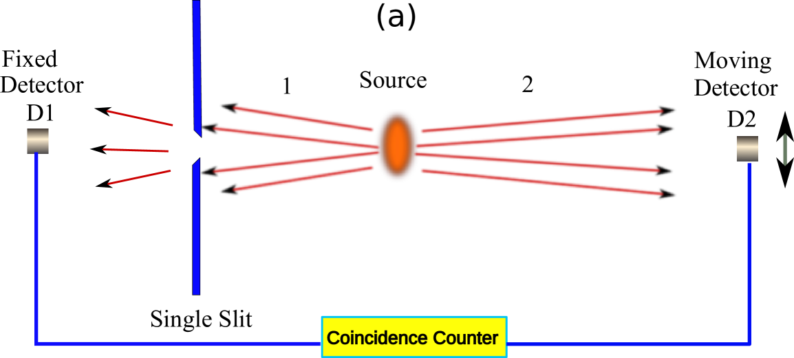
Figure 6: Schematic diagram of the Ghost diffraction experiment ghost . Detector D1 behind the slit is fixed, and the detector D1 sweeps up and down to capture photons. Detectors D1 and D2 count photons in coincidence. (a) Experiment with a single slit. (b) Experiment with a double-slit.

Let us look at the result of Strekalov et al’s experiment (see FIG. 7). The points represent the width of the diffraction pattern, in Strekalov et al’s experiment, as a function of the slit width. For small slit width, the width of the diffraction pattern sharply increases as the slit is narrowed. This is in clear contradiction with Popper’s prediction. To emphasize the point, we quote Popper: popper

“If the Copenhagen interpretation is correct, then such counters on the far side of B that are indicative of a wide scatter (and of a narrow slit) should now count coincidences: counters that did not count any particles before the slit at A was narrowed.”

Strekalov et al’s experiment shows exactly that, except that one is using a scanning D2 instead of an array of fixed detectors. So, we conclude that Popper’s test has decided in favor of Copenhagen interpretation.

Figure 7: Width of the diffraction pattern, plotted against the full width of slit A. The squares represent the data of Strekalov et al’s experiment ghost . The line represents the theoretical width, calculated from (17) for $\hbar/\sigma=0.04$ mm, using the parameters of Strekalov et al’s experiment

The theoretical analysis carried out by us should apply to Strekalov et al’s experiment, with the understanding that the single slit interference pattern is seen only if D1 is fixed. In other words, if D1 were also scanned along y-axis, the diffraction pattern would essentially remain the same except that the smaller peaks, indicative of interference from different regions within the slit, would be absent. We use (17) to plot the full width at half maximum of the diffraction pattern against, $2\epsilon$, which we assume to be the full width of the rectangular slit A (see FIG. 7). The plot uses $2L_{1}+L_{2}=1.8$ m, the value used in Ref. ghost , and an arbitrary $\hbar/\sigma=0.04$ mm. Our graph essentially agrees with that of Strekalov et al. Some deviation is there because we have not taken into account the beam geometry, and the finite size (0.5 mm) of the detectors, which will lead to an additional contribution to the width.

Our analysis led us to conclude that the virtual slit created for photon 2, in Popper’s experiment, is located not at slit B, but at slit A, a very counter-intuitive result. Strekalov et al also find that the virtual single-slit and the virtual double-slit for photon 2 are located at the slit which is in the path of photon 1. Thus our analysis agrees perfectly with their experimental results.

IX Discussion and conclusion

The indirect localization of particle 2 is not perfect in Kim and Shih’s experiment, but does it go against the Copenhagen interpretation, and agree with Popper’s viewpoint? The answer is no. As seen from our analysis, the width of the diffraction pattern for particle 2 given by (20), will always be smaller than the original width of the beam, however good the correlation between the two particles be. We emphasize again that by the original width of the beam we mean the spread of photons without doing any coincidence counting. With a real slit, of course, the diffraction width can be larger than the width of the original beam. This is exactly what was observed in Kim and Shih’s experiment. So, Popper’s thinking that Copenhagen interpretation implies that particle 2 will experience the same degree of diffraction as particle 1, is not correct. However, Popper alone cannot be blamed for this flawed assumption. All the defenders of Copenhagen interpretation seemed to have the same view, that is why nobody pointed otherwise, and that is the reason why there was so much surprise at the results of Kim and Shih’s experiment.

In our view, the only robust criticism of Popper’s experiment was that by Sudbery, who pointed out that in order to have perfect correlation between the two entangled particles, the momentum spread in the initial state, had to be truly infinite, which made any talk of additional spread, meaningless sudbery ; sudbery2 . For some reason, the implication of Sudbery’s point was not fully understood. It is this very point which, when generalized, leads to our conclusion that no additional momentum spread in particle 2 can be seen, even in principle.

We have shown that Strekalov et al’s ghost-diffraction experiment, actually implements Popper’s test in a conclusive way, but the result is in contradiction with Popper’s prediction. At actually shows that as slit A is narrowed, the other particle of the pair undergoes an increased diffraction, in coincident measurements. Popper was of the view that if the particles whose position has been indirectly measured to greater accuracy, shows an increased scatter, it could be interpreted as indicative of an action at a distance. From this point of view, we conclude that the Copenhagen interpretation has been vindicated. It could not have been otherwise, because our theoretical analysis shows that the results are a consequence of the formalism of quantum mechanics, and not of any particular interpretation.

Today we are in a position to sit back and reflect on why Popper’s experiment generated so much controversy. The problem was that Popper and most of his critics arrived at a wrong conclusion as to what result the experiment would yield. This was simply because no one cared to do a rigorous analysis, but used some commonly understood notions about measurement, which led them to a wrong conclusion. With a lot of theoretical and experimental work in quantum systems behind us, now we are wiser and realize that quantum mechanics is full of such pitfalls. Popper’s experiment has proved to be useful in understanding what quantum correlations are, and more importantly, what they are not.

References

- (1) “Can quantum-mechanical description of physical reality be considered complete?”, A. Einstein, B. Podolsky, N. Rosen, Phys. Rev. 47, 777-780 (1935),
- (2) K. R. Popper, Quantum Theory and the Schism in Physics (Hutchinson, London, 1982), pp. 27–29.
- (3) “Realism in quantum mechanics and a new version of the EPR experiment”, K.R. Popper, pp. 3-25, in Open Questions in Quantum Physics, edited by G. Tarozzi and A. van der Merwe (Dordrecht, Reidel, 1985)
- (4) “Popper’s variant of the EPR experiment does not test the Copenhagen interpretation”, A. Sudbery, Phil. Sci. 52, 470–476 (1985).
- (5) “Testing interpretations of quantum mechanics”, A. Sudbery in Microphysical Reality and Quantum Formalism, edited by A. van der Merwe et al (1988) pp 267-277.
- (6) “Popper, propensities, and the quantum theory”, H. Krips, Brit. J. Phil. Sci. 35, 253–274 (1984).
- (7) “Analysis of a proposed crucial test of quantum mechanics”, M.J. Collet, R. Loudon, Nature 326, 671–672 (1987).
- (8) “Measurement-induced diffraction and interference of atoms”, P. Storey, M.J. Collet, D. F. Walls, Phys. Rev. Lett. 68, 472–475 (1992).
- (9) “Popper and the quantum theory”, M. Redhead in Karl Popper: Philosophy and Problems, edited by A. O’Hear (Cambridge, 1996) pp 163-176.
- (10) “Atomic position localization via dual measurement”, H. Nha, J.-H. Lee, J.-S. Chang, K. An, Phys. Rev. A 65, 033827–033833 (2002).
- (11) “Karl Popper and the Copenhagen interpretation”, A. Peres, Studies in History and Philosophy of Science 33, 23 (2002).
- (12) “Realism in the realized Popper’s experiment”, G. Hunter, AIP Conference Proc. 646 (1), 243–248 (2002).
- (13) “Popper’s experiment revisited”, P. Sancho, Found. Phys. 32, 789-805 (2002).
- (14) “Popper’s experiment, Copenhagen interpretation and nonlocality”, T. Qureshi, Int. J. Quant. Inf. 2, 407-418 (2004).
- (15) K. Popper, “Popper versus Copenhagen,”, Nature 328, 675 (1987).
- (16) “On some implications of the local theory Th(g) and of Popper’s experiment”, T. D. Angelidis in Gravitation and Cosmology: From the Hubble Radius to the Planck Scale, eds. R.L. Amoroso, G. Hunter, M. Kafatos, J-P. Vigier (Kluwer: New York, 2002) pp. 525-536
- (17) “Optical imaging by means of two-photon quantum entanglement,” T. B. Pittman, Y. H. Shih, D. V. Strekalov, A. V. Sergienko, Phys. Rev. A 52, R3429 (1995).
- (18) “Opposite momenta lead to opposite directions”, A. Peres, Am. J. Phys. 68, 991-992 (2000).
- (19) “On Peres’ statement Opposite momenta lead to opposite directions”, W. Struyve, W.D. Baere, J.D. Neve, S.D. Weirdt, Found. Phys. 34, 963 (2004).
- (20) “Experimental realization of Popper’s experiment: violation of the uncertainty principle?”, Y.-H. Kim, Y. Shih, Found. Phys. 29, 1849-1861 (1999).
- (21) “Quantum entanglement: from Popper’s experiment to quantum eraser”, Y. Shih, Y.-H. Kim, Optics Commun. 179, 357-369 (2000).
- (22) R. Plaga, “An extension of Popper’s experiment can test interpretations of quantum mechanics,” Found. Phys. Lett. 13, 461 (2000).
- (23) “Popper’s experiment and conditional uncertainty relations”, A. J. Short, Found. Phys. Lett. 14, 275-284 (2001).
- (24) C.S. Unnikrishnan, “Proof of absence of spooky action at a distance in quantum correlations,” Pramana - J. Phys. 59, 295-301 (2002).
- (25) C.S. Unnikrishnan, “Is the quantum mechanical description of physical reality complete? Proposed resolution of the EPR puzzle,” Found. Phys. Lett. 15, 1-25 (2002).
- (26) “Understanding Popper’s experiment”, T. Qureshi, Am. J. Phys. 73, 541–544 (2005).
- (27) “Popper’s experiment and communication”, E. Gerjuoy, A.M. Sessler, Am. J. Phys. 74, 643 (2006).
- (28) “Experimental Realization of Einstein-Podolsky-Rosen-Bohm Gedankenexperiment: A New Violation of Bell’s Inequalities”, A. Aspect, P. Grangier, G. Roger, Phys. Rev. Lett. 49, 91-94 (1982).
- (29) “Coherence properties of entangled light beams generated by paramteric down-conversion: theory and experiment”, A. Joobeur, B. E. A. Saleh, T. S. Larchuk, M. C. Teich, Phys. Rev. A 53, 4360–4371 (1996).
- (30) “Analysis of Popper’s experiment and its realization”, T. Qureshi, Prog. Theor. Phys. 127, 645-656 (2012).
- (31) “Observation of two-photon ghost interference and diffraction”, D.V. Strekalov, A.V. Sergienko, D.N. Klyshko, Y.H. Shih, Phys. Rev. Lett. 74, 3600–3603 (1995).
- (32) “Ghost interference and quantum erasure”, P. Chingangbam, T. Qureshi, Prog. Theor. Phys. 127, 383-392 (2012).