Exploring shot noise and Laser Doppler imagery with heterodyne holography

Abstract

Heterodyne Holography is a variant of Digital Holography, where the optical frequencies of signal and reference arms can be freely adjusted by acousto-optic modulators. Heterodyne Holography is an extremely versatile and reliable holographic technique, which is able the reach the shot noise limit in sensitivity at very low levels of signal. Frequency tuning enables Heterodyne Holography to become a Laser Doppler imaging technique that is able to analyze various kinds of motion.

I Introduction

Heterodyne Holography (HH) [1, 2] is a variant of the Digital Holography technique (i.e. holography where the holographic film is replaced by a Digital camera) where the frequencies of the illumination beam (signal arm) and of the holographic reference beam (local oscillator arm) are freely adjusted thanks to Acousto-Optic Modulators (AOM). This technique is called Heterodyne Holography, because it can be viewed as an optical heterodyne detection, in which the detector is a multipixel detector (i.e. a camera) which acquires the heterodyne signal on all the pixels at the same time keeping trace of the pixel to pixel correlations. These correlations bring the holographic information that can be used for holographic reconstruction.

II Heterodyne holography

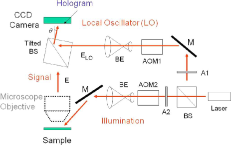
Figure 1: Digital holography setup. AOM1 and AOM2: Acousto-optic modulators; BS: Beam splitter; BE: Beam expander; M: Mirror; A1 and A2: Attenuator; $\theta$ : Tilt angle of the beam splitter with respect to optical axis.

A typical heterodyne holographic setup is presented on Fig.1. Thanks AOM1,and AOM2, the frequency $\omega_{LO}$ of the local oscillator field $E_{LO}$ and the frequency $\omega$ of the signal field $E$ are

$$\omega_{LO} = \omega_{L}+\omega_{AOM1}$$ (1)

$$\omega = \omega_{L}+\omega_{AOM2}$$

where $\omega_{L}$ is the main laser frequency, and $\omega_{AOM1,2}\simeq 80$MHz are the frequencies of the signals that drive AOM1 and AOM2.

This setup is extremely versatile and allows to perform either off-axis holography [3] or phase shifting holography [4]. For example, to perform a 4-phase detection, the frequency shift between the LO and signal beam must be chosen such as:

$$\omega_{LO}-\omega=\omega_{AOM1}-\omega_{AOM1}=\omega_{CCD}/4$$ (2)

where $\omega_{CCD}$ is the frame rate of the camera. In that case, the holographic signal $EE_{LO}^{*}$ is obtained by 4 phases demodulation of the camera signal. If $I_{n}$ where $n=0...3$ is the camera signal, and $n$ camera frame index, the holographic signal $EE_{LO}^{*}$ is then given by:

$$EE_{LO}^{*}=(I_{0}-I_{2})+j(I_{1}-I_{3})$$ (3)

where $j^{2}=-1$.

Here, by combining the frames with the 4-phase linear combination $(I_{0}-I_{2})+j(I_{1}-I_{3})$ of Eq.2, we tune the heterodyne receiver at frequency

$$\omega_{H}=\omega_{LO}-\omega_{CCD}/4$$ (4)

Because of Eq.2, $\omega_{H}$ is equal to $\omega$, and the heterodyne receiver is tuned at the signal frequency $\omega$. One of the advantage of method, used here to shift the phase (AOMs), is the accuracy of the $\pi/2$ phase shift that is applied to the reference beam, from one frame to the next [5]. As a consequence, the parasitic twin image [6] is minimized.

We must note that it is is possible to make another choice for the frequency offset $\omega_{LO}-\omega$. In that case, the holographic detector will be able to explore different frequency components, opening the way to Laser Doppler Holographic Imaging [7], and to Sideband Digital Holographic Imaging [8].

III Shot Noise Holography

Because the holographic signal results from the interference of the object complex field $E$ with a reference complex field $E_{LO}$, whose amplitude can be much larger (i.e. $E_{LO}\gg E$), it benefits of an optical heterodyne gain

$$G_{H}=\frac{|EE^{*}_{LO}|}{|E|^{2}}$$ (5)

and is thus potentially well-suited for the detection of signal fields $E$ of weak amplitude [9, 10].

To better analyze this effect, one must measure the camera signal in photoelectron (e) Units. In typical experimental conditions, the LO beam intensity is adjusted to be at half saturation of the camera. With a 12 bits camera, whose gain is $G\simeq 5$ e/DC (photoelectron per Digital Count), the LO beam signal is then

$$I_{n}\simeq|E_{LO}|^{2}\sim 2000~{}\textrm{DC}\simeq 10^{4}~{}\textrm{e}$$ (6)

per pixel, and the LO beam shot noise standard deviation is $\sqrt{I_{n}}\sim 100$.

For a weak signal of about 1 e per pixel, the heterodyne gain is $G\sim 100$. The 1 e heterodyne signal: $|EE^{*}_{LO}|\sim 100$ e, is thus equal to the LO beam shot noise, yielding SNR =1 (Signal to Noise Ratio). We must note here that the camera reading noise ($\simeq 20$ e), and the camera Analog Digital Converter quantization noise ($\simeq 5$ e) can be neglected with respect to the LO beam shot noise ($\sim 100$ e) [11].

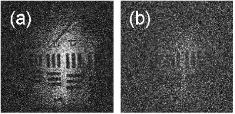
Figure 2: Reconstructed image of a USAF target from a sequence of $M=12$ images. The size of calculation grid (which is equal to the size of the recorded hologram) is $A_{calc}=1024\times 1024$ pixels. The size of the spatial filter [6] selected zone is $A_{calc}=400\times 400$ pixels. Average signal for $|E|^{2}$ is $\eta/M=0.0127$ (a), and $0.1\eta/M=0.00127$ e per pixel and per frame in (b), corresponding to $SNR\simeq 1$, and 0.1 respectively.

One can generalize this result for a sequence of $M$ images. One get that the shot noise limit, which corresponds to SNR =1, is reached for 1 e per pixel for the whole sequence of $M$ images, i.e. for $1/M$ e per pixel and per frame. One must notice also that the total amount of shot noise is proportional to the number of pixels (or spatial modes) that are used in the reconstruction procedure. If spatial filtering in the Fourier space is used [6], the shot noise must be multiplied by the ratio

$$\eta=A_{filter}/A_{calc}<1$$ (7)

where $A_{filter}$ is the number of pixels of the spatial filter in Fourier space, and $A_{calc}$ the number of pixels of the calculation grid. The shot noise limit corresponds thus to $\eta/M$ e per pixel and per frame [12].

Figure 2 shows, as an example, images of an USAF target that has been reconstructed from holographic data recorded at very low signal levels ($0.0127$ and $0.00127$ e per pixel and per frame in (a) and (b) respectively). These images illustrate the ability of heterodyne holography to reach the shot noise limit in low light with a standard array detector.

IV Laser Doppler Holography

IV-A Flows

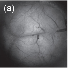
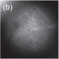
Figure 3: Image of a mouse crania reconstructed by Laser Doppler Holography: average of the intensity images reconstructed from data recorded with $\omega_{LO}-\omega$ varying from 36 to 48 Hz (a), and from 0.6 to 2.0 kHz (b).

The ability to control the frequency of the heterodyne detection $\omega_{H}$, following Eq.4, allow us to develop a Laser Doppler Holography. Thanks to the AOMs, we can adjust the frequency of the local oscillator $\omega_{LO}$ so as we can select a velocity component, whose optical frequency is $\omega_{H}$, and we can image it by holography [7]. It is also possible to reconstruct the images of the various velocity components by recording a sequence of images ($I_{1},I_{2}.....I_{n}$), and by making a time to frequency Fourier transformation [13, 14].

As the optical wavelength is much smaller than the ultrasound wavelength, this Laser Doppler Holography presents the advantage to allow the analyze flows in the $\mu m/s$ range [15]. This Laser Doppler Holography has been applied to the analysis of blood flow in capillaries. We have for example imaged cerebral blood flow in the micro vessels, in mice, in vivo [16, 17, 14]. The imaging is made in vivo, in minimally invasive conditions (the cranial skull remains present). Figure 4 gives an example of mouse cerebral blood flow images that can be obtained by this way. Similar results have been obtained on the retina of a rat [18].

IV-B Vibrations

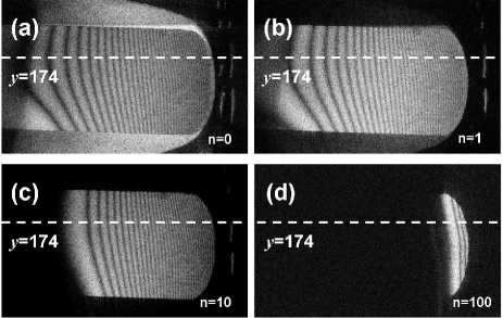
Figure 4: Reconstructed holographic images of a clarinet reed vibrating at frequency $\omega_{v}=2143$ Hz perpendicularly to the plane of the figure. Figure (a) shows carrier image obtained with $\omega_{H}=\omega$ ; Fig. (b)-(d) show the frequency sideband images obtained with $\omega_{H}=\omega+n\omega_{v}$, where $n$ the sideband harmonic order: $n=0$ (a), 1 (b), 10 (c) and 100 (d).

If the object vibrates periodically , the light that is reflected or diffracted by the object exhibit sidebands. It is then possible to tune the holographic heterodyne receiver at a sideband frequency [19, 8], and not simply at the carrier frequency like with standard digital holography [20]. If the amplitude of vibration is large, it is even possible to explore the whole comb of sideband lines, and to get, by the way, the map of the vibration amplitudes of the object. Figure 4 shows sideband images of a vibrating clarinet reed. Images with harmonic order up to $n\simeq 1200$ have been obtained by Heterodyne Holography [21].

V Conclusion

Heterodyne Holography is an extremely versatile and robust holographic technique, which is able to reach the shot noise limit of sensitivity in low light, and that is perfectly suited to the analysis of many modulation phenomena, flows or vibrations [17, 22, 23].

References

- [1] F. LeClerc, L. Collot, and M. Gross, “Numerical heterodyne holography using 2d photo-detector arrays,” Optics Letters, vol. 25, p. 716, Mai 2000.
- [2] F. Le Clerc, M. Gross, and L. Collot, “Synthetic-aperture experiment in the visible with on-axis digital heterodyne holography,” Optics Letters, vol. 26, no. 20, pp. 1550–1552, 2001.
- [3] U. Schnars and W. Juptner, “Digital recording and numerical reconstruction of holograms,” Measurement science and technology, vol. 13, no. 9, pp. 85–101, 2002.
- [4] I. Yamaguchi and T. Zhang, “Phase-shifting digital holography,” Optics Letters, vol. 18, no. 1, p. 31, 1997.
- [5] M. Atlan, M. Gross, and E. Absil, “Accurate phase-shifting digital interferometry,” Optics letters, vol. 32, no. 11, pp. 1456–1458, 2007.
- [6] E. Cuche, P. Marquet, and C. Depeursinge, “Spatial filtering for zero-order and twin-image elimination in digital off-axis holography,” Applied Optics, vol. 39, no. 23, pp. 4070–4075, 2000.
- [7] M. Atlan and M. Gross, “Laser Doppler imaging, revisited,” Review of Scientific Instruments, vol. 77, p. 116103, 2006.
- [8] F. Joud, F. Laloe, M. Atlan, J. Hare, and M. Gross, “Imaging a vibrating object by Sideband Digital Holography,” Optics Express, vol. 17, p. 2774, 2009.
- [9] F. Charrière, B. Rappaz, J. KŘhn, T. Colomb, P. Marquet, and C. Depeursinge, “Influence of shot noise on phase measurement accuracy in digital holographic microscopy,” Opt. Express, vol. 15, pp. 8818–8831, 2007.
- [10] F. Charrière, T. Colomb, F. Montfort, E. Cuche, P. Marquet, and C. Depeursinge, “Shot-noise influence on the reconstructed phase image signal-to-noise ratio in digital holographic microscopy,” Applied optics, vol. 45, no. 29, pp. 7667–7673, 2006.
- [11] M. Gross, M. Atlan, and E. Absil, “Noise and aliases in off-axis and phase-shifting holography,” Appl. Opt, vol. 47, pp. 1757–1766, 2008.
- [12] M. Gross and M. Atlan, “Digital holography with ultimate sensitivity,” Optics letters, vol. 32, no. 8, pp. 909–911, 2007.
- [13] M. Atlan and M. Gross, “Wide-field Fourier transform spectral imaging,” Applied Physics Letters, vol. 91, p. 113510, 2007.
- [14] M. Atlan, M. Gross, T. Vitalis, A. Rancillac, J. Rossier, and A. Boccara, “High-speed wave-mixing laser Doppler imaging in vivo,” Optics Letters, vol. 33, no. 8, pp. 842–844, 2008.
- [15] M. Atlan, M. Gross, and J. Leng, “Laser Doppler imaging of microflow,” J. Eur. Opt. Soc. Rapid Publications, vol. 1, p. 06025, 2006.
- [16] M. Atlan, M. Gross, B. Forget, T. Vitalis, A. Rancillac, and A. Dunn, “Frequency-domain wide-field laser Doppler in vivo imaging,” Optics letters, vol. 31, no. 18, pp. 2762–2764, 2006.
- [17] M. Atlan, B. Forget, A. Boccara, T. Vitalis, A. Rancillac, A. Dunn, and M. Gross, “Cortical blood flow assessment with frequency-domain laser Doppler microscopy,” Journal of Biomedical Optics, vol. 12, p. 024019, 2007.
- [18] M. Simonutti, M. Paques, J. Sahel, M. Gross, B. Samson, C. Magnain, and M. Atlan, “Holographic laser Doppler ophthalmoscopy,” Optics Letters, vol. 35, no. 12, pp. 1941–1943, 2010.
- [19] C. C. Aleksoff, “Temporally modulated holography,” Appl. Opt., vol. 10, no. 6, pp. 1329–1341, 1971.
- [20] P. Picart, J. Leval, D. Mounier, and S. Gougeon, “Time-averaged digital holography,” Optics letters, vol. 28, no. 20, pp. 1900–1902, 2003.
- [21] F. Joud, F. Verpillat, F. Laloë, M. Atlan, J. Hare, and M. Gross, “Fringe-free holographic measurements of large-amplitude vibrations,” Optics letters, vol. 34, no. 23, pp. 3698–3700, 2009.
- [22] T. Colomb, J. Kühn, F. Charriere, C. Depeursinge, P. Marquet, and N. Aspert, “Total aberrations compensation in digital holographic microscopy with a reference conjugated hologram.”
- [23] J. Kühn, F. Montfort, T. Colomb, B. Rappaz, C. Moratal, N. Pavillon, P. Marquet, and C. Depeursinge, “Submicrometer tomography of cells by multiple-wavelength digital holographic microscopy in reflection,” Optics letters, vol. 34, no. 5, pp. 653–655, 2009.