HATS-1b: The First Transiting Planet Discovered by the HATSouth Survey

Abstract

We report the discovery of HATS-1b, a transiting extrasolar planet orbiting the moderately bright V=$12.05$ G dwarf star GSC 6652-00186, and the first planet discovered by HATSouth, a global network of autonomous wide-field telescopes. HATS-1b has a period of $P\approx 3.4465$ d, mass of $M_{p}\approx 1.86$ $M_{\rm J}$, and radius of $R_{p}\approx 1.30$ $R_{\rm J}$. The host star has a mass of $0.99$ $M_{\sun}$, and radius of $1.04$ $R_{\sun}$. The discovery light curve of HATS-1b has near continuous coverage over several multi-day periods, demonstrating the power of using a global network of telescopes to discover transiting planets.

1. Introduction

The detection and study of extrasolar planets has become one of the fastest developing fields in astrophysics. This has been fueled by the extraordinarily rapid rate of exoplanetary discovery. The two most productive discovery techniques have been the radial velocity (RV) method (measuring the reflex RV signature of a planetary orbit in its parent star) and the transit method (measuring the slight decrease in stellar brightness that occurs if the planet happens to pass across its parent star’s disk as viewed from the Earth).

Even though among confirmed planets, much more were detected by the RV method than the transit method, the latter enables many studies that are not possible for RV detected planets, since for each transiting system a lot more information is available than for an RV only system, like the planet radius, an unambiguous mass and the inclination of the orbit relative to the line of sight.

In addition, observations and measurements are possible for transiting planets that cannot be done with RV-only planets. It is possible to measure the misalignment between stellar spin and planetary orbits through the Rossiter-McLaughlin (RM) effect (e.g., Queloz et al., 2000; Winn et al., 2005, 2006, 2007, 2008, 2009, 2010a, 2010b, 2011; Narita et al., 2007, 2008, 2009b, 2009a, 2010b, 2010a, and many others). Information can be obtained about the planetary atmosphere by measuring the dependence of the transit depth (planet radius) on wavelength (e.g., Charbonneau et al., 2002; Redfield et al., 2008; Snellen et al., 2008; Sing et al., 2008, 2009, 2011a, 2011b). The surface brightness and atmospheric temperature of the planet can be determined from observations of the secondary eclipse, when the planet goes behind the star, and from the out of eclipse variations in the combined planet plus star brightness (e.g., Snellen & Covino, 2007; Snellen et al., 2010; Deming et al., 2007, 2011; Charbonneau et al., 2008; Demory et al., 2012), as well as a wide array of other theoretical and observational studies.

For these reasons, increasing the sample of known transiting extrasolar planets, and extending the range of systems for which transits are detectable is very valuable. The HATSouth network, described in detail in Bakos et. al. (2012) (to be submitted), is designed to achieve both of these goals. With telescopes situated at three sites in the southern hemisphere, roughly $120^{\circ}$ apart in longitude, HATSouth is capable of detecting transits at longer periods than any other ground based network presently in operation. In addition, as detailed in Bakos et. al. (2012), it is one of the most sensitive wide–field, ground based searches to small planets. Since a large part of the sky is being surveyed, many bright stars will be checked for transits. As a consequence, the HATSouth survey is expected to find many of its planets around bright stars, which makes the detailed follow up studies mentioned above feasible.

In this paper we present the first planet to come from the HATSouth survey: HATS-1b. Since this is the first transiting planet discovered by th esurvey, we describe in detail the data analysis methods and the procedures used to confirm the planetary nature of the object and derive the stellar and planetary parameters.

The layout of the paper is as follows. In Section 2 we report the detection of the photometric signal and the follow-up spectroscopic and photometric observations of the host star, HATS-1. In Section 3 we describe the analysis of the data, beginning with the determination of the stellar parameters, continuing with a discussion of the methods used to rule out nonplanetary, false positive scenarios which could mimic the photometric and spectroscopic observations, and finishing with a description of our global modeling of the photometry and radial velocities. Our findings are discussed in Section 4.

2. Observations

2.1. Photometric detection

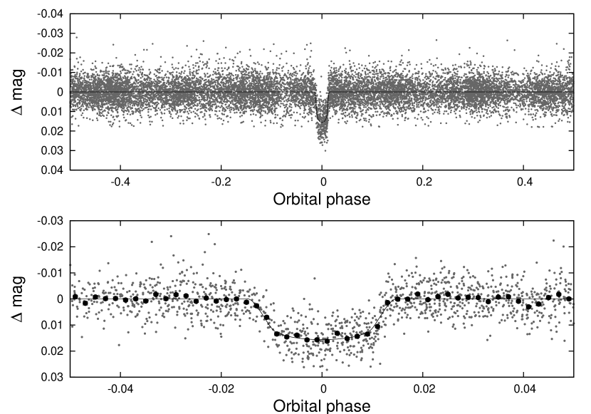
Figure 1.— Unbinned instrumental $r$-band light curve of HATS-1 folded with the period $P=3.4464588$ days resulting from the global fit described in Section 3. The solid line shows the best-fit transit model (see Section 3.3). In the lower panel we zoom-in on the transit; the dark filled points here show the light curve binned in phase using a bin-size of 0.002.

Table 1 Summary of photometric observations

Facility	Date(s)	Number of Images	Cadence (s)	Filter
HS-1	2010 Jan–2010 Aug	6018	276	Sloan $r$
HS-3	2010 Jan–2010 Aug	5391	281	Sloan $r$
HS-5	2010 Jan–2010 Aug	655	271	Sloan $r$
Swope/SITe3	2011 May 25	57	196	Sloan $i$
FTS/Spectral	2011 May 28	68	60	Sloan $r$
FTS/Spectral	2011 Jul 05	74	64	Sloan $i$
MPG/ESO2.2/GROND	2012 Jan 21	78	148	Sloan $g$
MPG/ESO2.2/GROND	2012 Jan 21	80	148	Sloan $r$
MPG/ESO2.2/GROND	2012 Jan 21	78	148	Sloan $i$

Table 1 summarizes the HATSouth discovery observations of HATS-1b. Observations were obtained over an eight month period from 2010 Jan through 2010 Aug using the HS1 (HATSouth 1) instrument in Chile, the HS3 instrument in Namibia, and the HS5 instrument in Australia. The observations, reduction, and analysis of the HATSouth data were carried out as described in Bakos et. al. (2012). We detected a significant transit signal in the light curve of GSC 6652-00186 (also known as 2MASS 11420608-2321174; $\alpha=11^{\mathrm{h}}42^{\mathrm{m}}06.12{\mathrm{s}}$, $\delta=-23{\arcdeg}21{\arcmin}17.4{\arcsec}$; J2000; V=$12.053\pm 0.017$ mag APASS DR5, e.g. Henden et al., 2009; see Figure 1).

2.2. Spectroscopy

Table 2 summarizes the follow-up spectroscopic observations which we obtained for HATS-1. Initial medium and low-resolution “reconnaissance” observations were obtained using the Wide Field Spectrograph (WiFeS; Dopita et al., 2007) on the ANU 2.3 m telescope. These observations were used to rule out various common false positive scenarios (blends between an eclipsing binary and a giant star, or F-M type binary systems). We then obtained higher resolution, and higher RV precision observations with the Coralie spectrograph on the Euler 1.2 m telescope at La Silla Observatory, FEROS on the MPG/ESO 2.2 m telescope at La Silla, FIES (Djupvik & Andersen, 2010) on the 2.5 m Nordic Optical Telescope, and CYCLOPS on the 3.9 m Anglo-Australian Telescope (AAT) at Siding Spring Observatory (SSO). Below we describe the observations and reduction techniques for each spectroscopic instrument used.

2.2.1 ANU 2.3 m/WiFeS

High signal to noise (S/N), medium resolution reconnaissance spectroscopy was performed with WiFeS on the ANU 2.3 m telescope. WiFeS is an image slicing integral field spectrograph with 25 slitlets each sampled at $0.5^{\prime\prime}$. Our observations, made with the red arm of the spectrograph, employed the R7000 grating and the RT480 dichroic, giving a spectral resolution of $\lambda/\Delta\lambda=7\,000$ and velocity dispersion of $21.6\,\rm km\,s^{-1}\,\text{pixel}^{-1}$ in the wavelength region $5\,200-7\,000\,\text{\AA}$. The $4\text{K}\times 4\text{K}$ CCD was read out in $2\times$ binning in the spatial direction, with a detector gain of $0.9\,e^{-}\,\text{ADU}^{-1}$, and read noise of $5\,e^{-}\,\text{s}^{-1}\,\text{pixel}^{-1}$. Only half the CCD containing the stellar signal was read out to reduce the readout time. RV standard star exposures were taken on each night during twilight.

Reduction of the spectra was performed using the IRAF package CCDPROC, and extracted in TWODSPEC. Spectra from the three brightest image slices were extracted individually. Wavelength calibrations were performed with bracketing Ne-Ar arc lamp exposures. Atmospheric Oxygen B band lines in the region $6\,882-6\,906\,\text{\AA}$ were used to provide a first order wavelength correction. Object spectra were cross correlated against RV standard star spectra in the wavelength region $5\,270-5\,650\,\text{\AA}$. Velocity measurements were obtained for each permutation of image slice and standard star spectra cross correlation, performed using the task FXCOR. The template and object spectra were Fourier filtered to remove low and high frequency noise, and a Gaussian fit was performed on the peak of the cross correlation function to derive the velocity shift. The final RV measurements were calculated as the mean of these velocities weighted according to the cross correlation function peak and object spectrum S/N.

The RV root mean square (RMS) scatter of multi-epoch WiFeS observations is $1\,\rm km\,s^{-1}$, as measured from RV standard stars. We scheduled our observations at orbital phase quadrature of the candidate, where the velocity difference is the greatest. The results from five observations (with mean exposure time of 400 s) show no RV variation greater than $2\,\rm km\,s^{-1}$, indicating that the candidate was not an unblended eclipsing binary.

We also obtained a single (700 s exposure) low resolution ($\lambda/\Delta\lambda=3\,000$) spectrum which was used to estimate $T_{\rm eff\star}$ and $\log{g_{\star}}$. We use the blue arm of WiFeS with the B3000 grating and RT560 dichroic, which gives a wavelength coverage of $3\,500-6\,000\,\text{\AA}$ at $\lambda/\Delta\lambda=3\,000$ resolution. Spectrophotometric standard stars from Hamuy et al. (1994) are observed for flux calibration, and a Ne-Ar lamp is used for wavelength calibration. Reductions are performed using the IRAF packages CCDPROC, KPNOSLIT and ONEDSPEC. The four brightest image slices are summed, and the object spectrum is divided by a black body white dwarf spectrum to remove the instrument sensitivity function. Flux calibration is performed according to the methodology set out in Bessell (1999). The spectrum is matched to a grid of synthetic MARCS model atmospheres (Gustafsson et al., 2008), fitting for $T_{\rm eff\star}$, $\log{g_{\star}}$, [Fe/H], and interstellar reddening ($E(B-V)$), at 250 K, 0.5 dex, and 0.01 magnitude intervals respectively. Regions sensitive to changes in $\log g$, such as the Balmer jump, the MgH feature at $4\,800\,\text{\AA}$, and the Mg b triplet at $5\,170\,\text{\AA}$, are weighted preferentially. Based on the approximate $\log{g_{\star}}$ and $T_{\rm eff\star}$, we find that HATS-1 is a dwarf.

2.2.2 Euler 1.2 m/Coralie

We used the CORALIE spectrograph mounted on the Swiss 1.2 m Leonard Euler telescope in the ESO La Silla Observatory to measure 6 radial velocities (RVs) for HATS-1b during a run on 2011 May 19-20. CORALIE is a fiber-fed Echelle spectrograph with a design similar to ELODIE (Baranne et al., 1996) and originally installed on April 1998 (Queloz et al., 2001). It was refurbished in 2007 to increase its optical efficiency; the refurbished instrument provides a resolution of $\sim 60\,000$. Spectra of our targets are taken in simultaneous Thorium-Argon (ThAr) mode, whereby one of the fibers observes the target and the other a ThAr lamp (hereafter the object and comparison fibers, respectively).

An automated pipeline was developed at Pontificia Universidad Católica de Chile to extract and calibrate the CORALIE spectra, following in large part the reduction scheme for ELODIE described in Baranne et al. (1996). We provide a brief description of the reduction procedure here, full details will be given elsewhere. A night of observations include the following sets of images: (i) science frames, where the object fiber observes the target and the comparison fiber is illuminated by the ThAr lamp; (ii) ThAr frames, where both fibers are illuminated by the ThAr lamp; (iii) flats, where each of the fibers in turn is illuminated by a lamp at the beginning of the night. The pipeline trims and bias subtracts all frames. Flats are then median combined and used to find and trace each of the Echelle orders; the traces are fit by polynomials of order 4 and stored for extraction of the ThAr and science frames. We extract 70 orders from the object fiber and 51 from the comparison one, the wavelength coverage of the object fiber is $\approx$3 850–6 900 Å. All ThAr frames are then extracted using the traces obtained from the flats, ThAr lines are identified and then fit by Gaussians. Only lines from the list of Lovis & Pepe (2007) are used. With the line centroids and wavelengths given in Lovis & Pepe (2007) in hand, a global (i.e., for all orders simultaneously) wavelength solution of the form $\lambda=P(x,m)/m$ is then fit, for the science and comparison fibers independently, where $x$ is pixel position of ThAr lines along the dispersion direction, $m$ is the Echelle order number and $P(x,m)$ is a polynomial of order 3 in $x$ and 5 in $m$. When fitting the wavelength solution we reject lines iteratively until the rms around the fit is acceptable.

The spectrum in each Echelle order of the object fiber in the science frames is extracted using the optimal extraction algorithm of Marsh (1989). The comparison ThAr spectra are extracted via a simple extraction and are used to calculate the velocity shift $\delta v$ of the comparison fiber of each science frame with respect to the comparison fiber of the ThAr frame nearest in time. The wavelength calibration for the orders corresponding to the object fiber in the science frames is done by applying the wavelength solution of the object fiber of the ThAr frame nearest in time shifted by $\delta v$. Finally, we apply a barycentric correction computed at the flux-weighted mean of the exposure and calculated using the JPL Solar System ephemeris. With the spectra calibrated and corrected to the barycenter of the Solar System, a cross-correlation function is calculated using a binary mask as described in Baranne et al. (1996). A spectral typing module within the pipeline gives estimates of $T_{\rm eff}$, $\log(g)$, $v\sin(i)$ and [Fe/H] for each target, and we use these to choose an appropriate cross-correlation mask within a set of three choices: G2, K5, M2. The resulting CCF is fit with a Gaussian and the mean returned by the fit is the measured RV. Following Queloz (1995) we estimate the uncertainty in the measured RVs via the scaling $\sigma_{\rm RV}=a+[(1.6+0.2w)b/sn]$, where $sn$ is the signal-to-noise ratio at 5 130 Å , $w$ is the width of the CCF measured in pixels, and $a\approx 6$ $\rm m\,s^{-1}$ and $b\approx 100$ $\rm m\,s^{-1}$ are constants that are determined via simulations and depend slightly on spectral type. We have monitored the RV standard HD 72673 for $\approx$ 2 years, obtaining 40 RV measurements with S/N$>$60 per pixel at 5 130 Å. This star is known to have a long-term RV rms of $\sim 2$ $\rm m\,s^{-1}$ from HIRES/Keck observations (Andrew Howard, private communication). Our CORALIE RV measurements have an RMS of 8 $\rm m\,s^{-1}$, which showcases the long-term velocity precision we can currently achieve with CORALIE for bright targets. The observations of HD 72673 show that even at high S/N we do not reach the level implied by the constant $a$ in the expression for $\sigma_{\rm RV}$ but rather we are limited to $\sigma_{\rm RV,min}=8$ $\rm m\,s^{-1}$, which we adopt as our lower limit in the velocity uncertainty estimates.

2.2.3 NOT 2.5 m/FIES

We obtained two observations of HATS-1 using the FIbre-fed Échelle Spectrograph (FIES) on the 2.5 m Nordic Optical Telescope (NOT) located on the island of La Palma (Djupvik & Andersen, 2010). The FIES observations were reduced to spectra following the procedure of Buchhave et al. (2010). We used these spectra to measure the atmospheric parameters of HATS-1, including the effective temperature $T_{\rm eff\star}$, the metallicity $\rm[Fe/H]$, the projected rotational velocity $v\sin{i}$, and the stellar surface gravity $\log{g_{\star}}$, by cross-correlating the observations against a finely sampled grid of synthetic spectra based on Kurucz (2005) model atmospheres. The procedure, called Stellar Parameter Classification (SPC), will be described in detail in a forthcoming paper (Buchhave et al., in preparation, see also Bakos et al., 2012 for results for other stars based on this method).

2.2.4 ESO 2.2 m/FEROS

Table 2 Summary of spectroscopic observations

Telescope/Instrument	Date Range	Number of Observations	Resolution
ANU 2.3 m/WiFeS	2011 May 10—15	5	7 000
ANU 2.3 m/WiFeS	2011 June 05	1	3 000
AAT 3.9 m/CYCLOPS	2012 Jan 5—12	6	70 000
Euler 1.2 m/Coralie	2011 May 19—20	6	60 000
NOT 2.5 m/FIES	2011 June 15—18	2	67 000
MPG/ESO 2.2 m/FEROS	2011 June 08— 2012 April 18	21	48 000

Figure 2.— Top panel: High-precision RV measurements for HATS-1 from CORALIE (dark filled circles), FEROS (open triangles) and CYCLOPS (filled triangles) shown as a function of orbital phase, together with our best-fit model. Zero phase corresponds to the time of mid-transit. The center-of-mass velocity has been subtracted. Second panel: Velocity $O\!-\!C$ residuals from the best fit. The error bars include a component from astrophysical/instrumental jitter allowed to differ for the three instruments. Third panel: Bisector spans (BS), with the mean value subtracted. Note the different vertical scales of the panels.

Table 3 Relative radial velocities and bisector span measurements of HATS-1.

BJD	RV	$\sigma_{\rm RV}$	BS	$\sigma_{\rm BS}$	Phase	Instrument
(2 454 000$+$)	($\rm m\,s^{-1}$)	($\rm m\,s^{-1}$)	($\rm m\,s^{-1}$)
$1701.46966$	$64.78$	$24.00$	$30.4$	$84.4$	$0.523$	Coralie
$1701.49218$	$53.78$	$25.00$	$103.3$	$87.4$	$0.530$	Coralie
$1701.67397$	$132.78$	$28.00$	$3.7$	$105.8$	$0.583$	Coralie
$1701.69858$	$132.78$	$29.00$	$0.2$	$140.7$	$0.590$	Coralie
$1702.46676$	$229.78$	$23.00$	$-312.9$	$87.2$	$0.813$	Coralie
$1702.49046$	$209.78$	$23.00$	$2.7$	$64.3$	$0.819$	Coralie
$1721.48200$	$-190.09$	$61.09$	$-193.4$	$257.4$	$0.330$	FEROS
$1722.56100$	$246.23$	$53.72$	$97.1$	$53.8$	$0.643$	FEROS
$1723.60400$	$28.04$	$59.75$	$-10.1$	$100.3$	$0.946$	FEROS
$1724.61100$	$-409.37$	$58.84$	$-350.1$	$98.5$	$0.238$	FEROS
$1726.63000$	$157.47$	$47.67$	$-85.7$	$139.2$	$0.824$	FEROS
$1728.53900$	$-146.13$	$56.44$	$-263.5$	$117.4$	$0.377$	FEROS
$1735.51300$	$-121.06$	$81.73$	$-130.1$	$514.8$	$0.401$	FEROS
$1736.57100$	$286.48$	$50.45$	$30.3$	$63.6$	$0.708$	FEROS
$1737.46400$	$75.76$	$50.47$	$14.1$	$70.5$	$0.967$	FEROS
$1738.46000$	$-90.05$	$57.78$	$-46.1$	$72.1$	$0.256$	FEROS
$1901.84000$	$281.61$	$34.46$	$55.4$	$129.7$	$0.661$	FEROS
$1911.84100$	$79.18$	$39.24$	$236.8$	$493.2$	$0.563$	FEROS
$1932.13480$	$-2.80$	$39.60$	$-240.8$	$57.8$	$0.451$	CYCLOPS
$1933.09769$	$-104.80$	$115.00$	$-49.3$	$279.6$	$0.731$	CYCLOPS
$1933.18812$	$208.10$	$33.62$	$283.5$	$59.9$	$0.757$	CYCLOPS
$1936.86700$	$274.56$	$48.03$	$37.1$	$49.0$	$0.824$	FEROS
$1938.16979$	$-265.20$	$21.28$	$6.0$	$66.2$	$0.202$	CYCLOPS
$1939.19224$	$-22.00$	$15.65$	$1.6$	$45.9$	$0.499$	CYCLOPS
$1943.22390$	$271.60$	$17.65$	$-0.9$	$22.0$	$0.669$	CYCLOPS
$1991.75100$	$108.73$	$56.55$	$-19.4$	$65.4$	$0.749$	FEROS
$2021.75000$	$-33.57$	$57.03$	$105.1$	$42.7$	$0.453$	FEROS
$2024.79300$	$-50.14$	$90.16$	$76.1$	$160.6$	$0.336$	FEROS
$2025.78200$	$222.49$	$46.75$	$54.7$	$64.5$	$0.623$	FEROS
$2029.73900$	$163.37$	$65.29$	$-189.6$	$192.5$	$0.772$	FEROS
$2031.54600$	$-256.83$	$46.88$	$197.9$	$161.3$	$0.296$	FEROS
$2032.70200$	$81.66$	$40.39$	$-77.7$	$130.8$	$0.631$	FEROS
$2035.65100$	$27.54$	$69.87$	$35.9$	$72.2$	$0.487$	FEROS

[-1.5ex]

FEROS is the “Fiber-fed Extended Range Optical Spectrograph” located at the 2.2 m MPG/ESO telescope at the La Silla Observatory, Chile. The instrument covers the whole wavelength range between 3 500 and 9 200 Å separated into 39 spectral orders at a resolving power $\lambda/\Delta\lambda$ of 48 000 (Kaufer & Pasquini, 1998), making the analysis of the radial velocity and activity indicators such as Ca II H and K simultaneously possible (Setiawan et al., 2003).

FEROS is equipped with a double fiber system, providing the opportunity to observe in object-sky or in object-calibration mode. The observations for HATS-1 were taken in the object-calibration mode to guarantee the highest achievable precision with FEROS. In this mode, a ThAr+Ne lamp spectrum is recorded parallel to the target exposure, in order to calibrate the wavelength simultaneously. This method is modeled on the ELODIE spectrograph (Baranne et al., 1996).

Kaufer & Pasquini (1998) report in the commissioning of FEROS at the 1.52 m telescope at La Silla observatory, Chile, a RV measurement error of $\sim$23 $\rm m\,s^{-1}$. An improved data reduction method (Setiawan et al., 2000), reduced this error to $\sim$10 m/s, enabling FEROS to be used for planet searches.

Between June 2011 and April 2012, a total of 21 spectra of HATS-1 were taken with FEROS during MPI guaranteed time (PI M. Mohler) and Chilean time (PI A. Jordán).

The data reduction, including bias- and flatfield-correction, wavelength calibration and barycentric motion correction, was done using the MIDAS data reduction pipeline at the telescope.

The radial velocity of each spectrum was calculated by cross-correlating the object spectrum with a synthetic one, generated with the program SPECTRUM (Gray & Corbally, 1994) using Kurucz models (Kurucz, 1993). In order to find the stellar parameters to synthesize the fitting spectrum for cross-correlation, the object spectra were analyzed using the program SME (Spectroscopy Made Easy, Valenti & Piskunov (1996)). Since the instrument efficiency of FEROS drops significantly below 4 000 Å and above $\sim$7 900 Å, only the spectral range between these limits was used for cross-correlation. Due to the fact that Balmer lines, areas of telluric lines and strong emission features can falsify the result, these areas were carefully excluded in the analysis. In total, 26 out of 39 orders were used. The RV was determined by fitting a Gaussian function to the final cross-correlation, with the center of the Gaussian fit representing the RV of the star.

2.2.5 AAT 3.9 m/CYCLOPS

High-precision radial velocity observations were obtained with the CYCLOPS fiber-system feeding the UCLES spectrograph on the 3.9 m AAT at SSO, Australia. UCLES is a cross-dispersed Echelle spectrograph located at the coudé focus with a 79 l mm^-1 grating. CYCLOPS is a Cassegrain fiber-based integral field unit used to feed UCLES. It consists of a 15 element fiber bundle which re-formats a $\sim 3^{\prime\prime}$ diameter aperture into a pseudo–slit $0.63^{\prime\prime}$ wide and 15 elements long. It delivers a spectral resolution of $\lambda/\Delta\lambda\sim 70\,000$ over 19 Echelle orders, with a total wavelength range of $4\,540-7\,340\,\mathrm{\AA}$.

The EEV2 $2\mathrm{K}\times 4\mathrm{K}$ CCD is readout with $\times 2$ binning in the spatial direction and the normal readout speed, delivering $1.3\,e^{-}\,\mathrm{ADU}^{-1}$ gain and a read-noise of $3.19\,e^{-}\,\mathrm{pix}^{-1}$. Exposure times vary between 1 200 s and 2 400 s depending on the brightness of the target and the weather conditions. We take a ThAr exposure before and after each science exposure to monitor the stability of the spectrograph.

Data reduction is performed using custom MATLAB routines, which trace each fiber and optimally extract each spectral order. Wavelength calibration is performed by linear interpolation between the ThAr exposures on either side of the exposure. Using the IRAF task FXCOR we cross-correlate each of the individual fiber spectra against corresponding fiber spectra of a very high signal-to-noise radial velocity standard star exposure. Final velocities are determined as the weighted mean of all fibers over all orders with 3 sigma clipping. Typically 12 fibers over 17 orders are used, with the two reddest orders too heavily contaminated with telluric lines to deliver precise RV measurements. RV uncertainties are calculated as the standard deviation of the scatter of the fibers over all the orders used.

2.3. Photometric follow-up observations

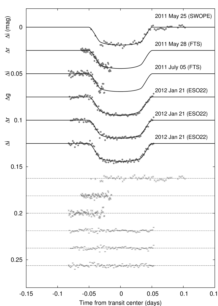
Figure 3.— Unbinned instrumental Sloan $g$-, $r$-, and $i$-band transit light curves of HATS-1. The dates and instruments used for each event are indicated. The light curves have been detrended using the EPD and TFA processes. Curves after the first are shifted for clarity. Our best fit is shown by the solid lines. Residuals from the fits are displayed at the bottom, in the same order as the top curves.

Follow-up photometric observations of HATS-1 were obtained using the SITe3 camera on the Swope 1.0 m telescope at LCO, the Spectral instrument on the 2.0 m Faulkes Telescope South (FTS) at SSO, and GROND on the MPG/ESO 2.2 m telescope at La Silla Observatory in Chile. Table 1 summarizes these observations. Below we describe the reduction procedures for each instrument used.

2.3.1 Swope 1 m/SITe3

The SITe#3 camera on the Swope 1 m telescope is a 2048$\times$3150 detector with a pixel scale of $0.435^{\prime\prime}$ and a field of view of $14.8^{\prime}\times 22.8^{\prime}$. Observations of a field centered on HATS-1 were calibrated using standard methods and reduced to light curves following a similar procedure to that used by Bakos et al. (2010) in the analysis of photometric follow-up data for the HATNet project. Briefly, we use a variation of the fitsh package (Pál, 2012) to identify sources on the images, cross-match them between images, perform aperture photometry on the images using a range of apertures, collect light curves for the detected sources, and perform an ensemble magnitude fit to correct the light curves for variations that are common to multiple sources. Auxiliary parameters describing the shape of the stellar profile, the position of each source on each image, the sky background, and the local variation in the sky background, are also recorded. These are used in the light curve fitting procedure (§ 3.3) to correct for systematic variations in the target star that are not removed by the ensemble magnitude fit.

2.3.2 FTS 2 m/Spectral

Two partial transits of HATS-1b were observed with the FTS, which is part of the Las Cumbres Global Telescope (LCOGT) Network. We used the 4K$\times$4K “Spectral” imaging camera, featuring $0.15^{\prime\prime}$ pixels and a $10^{\prime}$ FoV. Exposures of 40 s were taken in both $r$-band (2011 May 28) and $i$-band (2011 July 5), binning $2\times 2$ to reduce readout time, and slightly de-focusing the telescope to avoid saturation. Raw data is reduced via the automated reduction pipeline provided by LCOGT for FTS data. Photometry is performed by an automated pipeline based on Source Extractor (Bertin & Arnouts, 1996) aperture photometry and calibrated using selected neighboring reference stars. Details of these observations are set out in Table 2.3.3, and photometry of the two transit ingresses observed is presented in Figure 1.

2.3.3 ESO 2.2 m/GROND

A complete transit of HATS-1b was observed on UT 2012 January 21 in the Sloan g ($\lambda=4\,550$ Å), r ($\lambda=6\,270$ Å) and i-band ($\lambda=7\,630$ Å) of the GROND instrument (Greiner et al., 2008), mounted on the MPG/ESO 2.2 m telescope at the ESO La Silla Observatory (Chile). The simultaneous multiband time series was obtained applying a moderate telescope defocus to minimize flat-fielding errors and to avoid saturation due to abrupt seeing decrease. The field-of-view (FOV) of GROND in the three optical channels is $5.4^{\prime}\times 5.4^{\prime}$ with a pixel scale of $0.158^{\prime\prime}$ $\rm{pixel^{-1}}$, which allowed monitoring of the target and a few nearby reference stars. We acquired data for nearly 3.5 hr time interval, covering the predicted transit of HATS-1b.

The data reduction and analysis of the photometric data was performed using a customized pipeline, following standard procedures. The masterbias and masterflat frames were used to perform debias and flat-fielding of the science images. DAOPHOT aperture photometry was performed as implemented in the IDL APER function to obtain light curves of HATS-1 and the reference stars in GROND’s FOV with three aperture radii (27.5, 30 and 32.5 pixels). Finally a differential photometry was performed relative to the reference stars.

Table 4Differential photometry of HATS-1

Note. — This table is available in a machine-readable form in the online journal. A portion is shown here for guidance regarding its form and content.

3. Analysis

3.1. Properties of the parent star

As mentioned in Section 2.2.3 we determine the atmospheric parameters of the host star HATS-1, including the effective temperature $T_{\rm eff\star}$, the metallicity $\rm[Fe/H]$, the projected rotational velocity $v\sin{i}$, and the stellar surface gravity $\log{g_{\star}}$, by applying SPC to the FIES observations of this star. This analysis yielded the following initial values and uncertainties: $T_{\rm eff\star}=5870\pm 100$ K, $\rm[Fe/H]=-0.06\pm 0.12$ dex, $v\sin{i}=2.52\pm 0.5\,\rm km\,s^{-1}$, and $\log{g_{\star}}=4.52\pm 0.15$ (cgs).

The same parameters were independently determined by applying SME to the FEROS observations. The values obtained were $T_{\rm eff\star}=5790\pm 120$ K, $\rm[Fe/H]=-0.11\pm 0.1$ dex, $v\sin{i}=4.8\pm 0.5,\rm km\,s^{-1}$, and $\log{g_{\star}}=4.53\pm 0.17$ (cgs). These measurements, apart from $v\sin{i}$ are consistent within the quoted error bars. For the remainder of the paper the SPC results are adopted. The apparent inconsistency in the projected stellar rotation velocity is likely due to the mis–estimation of the quoted errors. For such slowly rotating stars, the uncertainties in both measurements are significantly larger than $0.5\,\rm km\,s^{-1}$.

Following Sozzetti et al. (2007) we use the stellar mean density $\rho_{\star}$, together with $T_{\rm eff\star}$ and $\rm[Fe/H]$ from SPC to constrain the fundamental properties of the star (mass, radius, age and luminosity) based on the Yonsei-Yale (Y2; Yi et al., 2001) stellar evolution models. The stellar mean density is closely related to the normalized semimajor axis $a/R_{\star}$, and is determined by modeling the light curve (§ 3.3). The light curve model also depends on the quadratic limb darkening coefficients, which we initially fix to the values from the Claret (2004) law using the initial $T_{\rm eff\star}$, $\rm[Fe/H]$, and $\log{g_{\star}}$ values. The comparison with the stellar evolution models provides a more precise estimate of $\log{g_{\star}}$ than can be determined from the spectrum. We we then fix $\log{g_{\star}}$ to this more precise value in a second iteration of SPC to determine revised estimates of the other atmospheric parameters ($T_{\rm eff\star}$, $\rm[Fe/H]$, and $v\sin{i}$). These new atmospheric parameters are used to determine new estimates of the limb darkening coefficients, which are used in a second iteration of the light curve modeling. We find that the value of $\log{g_{\star}}$ converges after two iterations.

We collect the final values for the observed and derived stellar parameters for HATS-1 in Table 5. The inferred location of the star in a diagram of $a/R_{\star}$ versus $T_{\rm eff\star}$, analogous to the classical H-R diagram, is shown in Figure 4. The stellar properties and their 1$\sigma$ and 2$\sigma$ confidence ellipsoids are displayed against the backdrop of Yi et al. (2001) isochrones for the measured metallicity of $\rm[Fe/H]$ = $-0.1$, and a range of ages.

Figure 4.— Model isochrones from Yi et al. (2001) for the measured metallicity of HATS-1, $\rm[Fe/H]$= $-0.1$, and ages of 0.2 Gyr, and 1 to 13 Gyr in 1 Gyr increments (left to right). The adopted values of $T_{\rm eff\star}$ and $a/R_{\star}$ are shown together with their 1$\sigma$ and 2$\sigma$ confidence ellipsoids. The open triangle shows the values from the initial SPC iteration.

Table 5 Stellar parameters for HATS-1

Parameter	Value	Source
Spectroscopic properties
$T_{\rm eff\star}$ (K)	$5870\pm 100$	SPC
$\rm[Fe/H]$	$-0.06\pm 0.12$	SPC
$v\sin{i}$ ($\rm km\,s^{-1}$)	$2.52\pm 0.5$	SPC
Photometric properties
$V$ (mag)	$12.053\pm 0.017$	APASS
$B$ (mag)	$12.740\pm 0.066$	APASS
$g$ (mag)	$12.356\pm 0.052$	APASS
$r$ (mag)	$11.866\pm 0.045$	APASS
$i$ (mag)	$11.748\pm 0.042$	APASS
$J$ (mag)	$10.924\pm 0.024$	2MASS
$H$ (mag)	$10.634\pm 0.022$	2MASS
$K_{s}$ (mag)	$10.580\pm 0.023$	2MASS
Derived properties
$M_{\star}$ ($M_{\sun}$)	$0.986\pm 0.054$	YY+$a/R_{\star}$+SPC
$R_{\star}$ ($R_{\sun}$)	$1.038_{-0.075}^{+0.128}$	YY+$a/R_{\star}$+SPC
$\log{g_{\star}}$ (cgs)	$4.40\pm 0.08$	YY+$a/R_{\star}$+SPC
$L_{\star}$ ($L_{\sun}$)	$1.10_{-0.18}^{+0.33}$	YY+$a/R_{\star}$+SPC
$M_{V}$ (mag)	$4.73\pm 0.24$	YY+$a/R_{\star}$+SPC
$M_{K}$ (mag,ESO)	$3.21\pm 0.22$	YY+$a/R_{\star}$+SPC
Age (Gyr)	$6.0\pm 2.8$	YY+$a/R_{\star}$+SPC
Distance (pc)	$303_{-23}^{+38}$	YY+$a/R_{\star}$+SPC

3.2. Excluding blend scenarios

Most of the obvious astrophysical false positive scenarios which might produce the detected transit of HATS-1 are ruled out by the spectroscopic observations discussed in Section 2.2. Some scenarios involving diluted eclipsing binary systems, or transiting planet systems diluted by an additional star, may still be consistent with these observations. To rule these scenarios out we conduct detailed modeling of the light curves following the procedure described in Hartman et al. (2011).

From the light curves alone we are able to rule out hierarchical triple star systems with greater than $4\sigma$ confidence, and blends between a foreground star and a background eclipsing binary with $\gtrsim 2.5\sigma$ confidence. Moreover, the only nonplanetary blend scenarios which could plausibly fit the light curves (scenarios for which the rejection confidence is less than $5\sigma$) are scenarios in which the two brightest stars in the blended system are nearly equal in brightness; such scenarios would have been easily detected from the spectroscopic observations (the spectrum would have either been obviously double-lined, or there would have been several $\rm km\,s^{-1}$ changes in the RV, BS, and/or FWHM; the latter is computed, and checked for variations, but not shown).

While our analysis rules out nonplanetary explanations for the observations, we are unable to disprove the possibility that the object is an unresolved stellar binary system (or chance alignment of two stars) with one component hosting a transiting planet. If this is the case the true mass and radius of the planet would be larger than what we infer. However, lacking any positive evidence for multiple stellar components in the system, for the analysis conducted in Section 3.3 we assume that HATS-1 consists of a single star with a transiting planet.

3.3. Global modeling of the data

We conducted a joint modeling of the HATSouth photometry, follow-up photometry, and RV data following the procedure described by Bakos et al. (2010). Briefly, we modeled the light curves using analytic formulae based on Mandel & Agol (2002) to describe the physical variation together with EPD and TFA to describe instrumental variations, and we modeled the RV data with a Keplerian orbit with the formalism of Pál (2009). We used the Downhill Simplex Algorithm (e.g. Press et al., 1992) to optimize the parameters, followed by a Markov-Chain Monte Carlo analysis (MCMC, e.g. Ford, 2006) to determine their uncertainties and correlations. The resulting geometric parameters pertaining to the light curves and velocity curves, as well as the derived physical planetary parameters, are listed in Table 6.

Included in this table is the RV “jitter” which was added in quadrature to the formal RV errors for the FEROS observations, such that $\chi^{2}/{\rm dof}=1$ for this instrument. The origin of this noise is unknown, it may either be to due astrophysical noise intrinsic to the star (potentially including additional planets in the system), or instrumental errors not included in the formal uncertainties.

We find that the planet has a mass of $M_{p}=1.855_{-0.196}^{+0.262}\,M_{\rm J}$ and radius of $R_{p}=1.302_{-0.098}^{+0.162}\,R_{\rm J}$, which are typical values for a hot Jupiter. We allow the eccentricity to vary in the fit so as to allow our uncertainty on this parameter to be included in the uncertainties of the other physical parameters of the system, however we find $e=0.120\pm 0.092$, which is consistent with zero eccentricity. Our $99\%$ upper-limit on the eccentricity is $e<0.4$.

Table 6Orbital and planetary parameters

Parameter	Value
Light curve parameters
$P$ (days)	$3.446459\pm 0.000004$
$T_{c}$ (${\rm BJD}$)	$2455241.28722\pm 0.00071$
$T_{14}$ (days)	$0.1007\pm 0.0012$
$T_{12}=T_{34}$ (days)	$0.0181\pm 0.0011$
$a/R_{\star}$	$9.20\pm 0.82$
$\zeta/R_{\star}$	$23.98\pm 0.16$
$R_{p}/R_{\star}$	$0.1288\pm 0.0020$
$b\equiv a\cos i/R_{\star}$	$0.633_{-0.023}^{+0.020}$
$i$ (deg)	$85.6_{-1.4}^{+0.6}$
Limb-darkening coefficients
$a_{g}$ (linear term)	$0.5230$
$b_{g}$ (quadratic term)	$0.2574$
$a_{r}$	$0.3387$
$b_{r}$	$0.3343$
$a_{i}$	$0.2560$
$b_{i}$	$0.3331$
RV parameters
$K$ ($\rm m\,s^{-1}$)	$254.1\pm 33.1$
$e\cos\omega$	$-0.064_{-0.064}^{+0.041}$
$e\sin\omega$	$0.097_{-0.073}^{+0.102}$
$e$	$0.120\pm 0.092$
RV jitter ($\rm m\,s^{-1}$)	$61.5$
Planetary parameters
$M_{p}$ ($M_{\rm J}$)	$1.855_{-0.196}^{+0.262}$
$R_{p}$ ($R_{\rm J}$)	$1.302_{-0.098}^{+0.162}$
$C(M_{p},R_{p})$	$0.53$
$\rho_{p}$ ($\rm g\,cm^{-3}$)	$1.03\pm 0.25$
$\log g_{p}$ (cgs)	$3.43\pm 0.07$
$a$ (AU)	$0.0444\pm 0.0008$
$T_{\rm eq}$ (K)	$1359_{-59}^{+89}$
$\Theta$	$0.127\pm 0.014$
$\langle F\rangle$ ($10^{8}$$\rm erg\,s^{-1}\,cm^{-2}$)	$7.70_{-1.22}^{+2.42}$

4. Discussion

The HATSouth global network of telescopes relies on combining observations from three stations located at three different sites in the southern hemisphere, with a close to optimal longitude separations. This makes it possible to continuously (or nearly so if the night is short) observe a given portion of the sky to search for transits of planets in front of their parent stars.

In this paper we have presented the first planet discovered by the HATSouth network. This discovery demonstrates that we are indeed able to successfully combine observations from multiple telescopes and sites to detect planetary transit signals.

In many respects this is a very typical transiting planet, with an orbital period of $P\approx 3.4465$ days (close to the mode for transiting planets detected from the ground), mass $M_{p}\approx 1.86$ $M_{\rm J}$ (slightly higher than typical), radius $R_{p}\approx 1.30$ $R_{\rm J}$ (close to the median for its mass), around a star that is an almost exact analogue of the Sun.

Figure 5 demonstrates the power of using a network of telescopes to search for transit signals among stars. It shows a ten day period (starting 2010 February 15) from the HATSouth discovery light curve containing 1351 observations of HATS-1, i.e. a small fraction of the total of more than 12 000 observations. Over this period, a significant fraction of the observations come from each of the three HATSouth sites, and a transit is detected by each station at a comparable significance. Despite the short nights in the southern hemisphere at this time, near continuous coverage is achieved and every single transit in this time window is observed by the HATSouth network. In contrast, a search operating from a single location would only be able to detect one of these transits.

As discussed in Bakos et. al. (2012) this increased duty cycle should result in many more planet detections, especially at longer periods and for smaller planetary radii, which are arguably the most valuable.

In Bakos et. al. (2012) detailed simulations were carried out showing that the distribution of planets expected to be produced by the HATSouth survey peaks at planet radii between 1 and 2 Jupiter radii and orbits with periods between 3 and 5 days. Not surprisingly, the first planetary system discovered by the network falls within these ranges. However, as discussed in that paper, these predicted distributions predict significantly enhanced sensitivity to planets with much longer orbital periods and smaller radii compared to a single site survey.

Figure 5.— (Left): The deviations of the measured brightness of HATS-1 from the median measured in magnitudes as a function of time in days. The different symbols denote observations from different sites/stations: pluses from LCO, circles from HESS and triangles from SSO. (Right): The same plot, but this time phase folded and zoomed in around the transit, occurring at phase of 0.5.

References

- Bakos et al. (2010) Bakos, G. Á., Torres, G., Pál, A., et al. 2010, ApJ, 710, 1724
- Bakos et al. (2012) Bakos, G. Á., Hartman, J. D., Torres, G., et al. 2012, arXiv: 1201.0659
- Bakos et. al. (2012) Bakos et. al. 2012
- Baranne et al. (1996) Baranne, A., Queloz, D., Mayor, M., et al. 1996, A&AS, 119, 373
- Bertin & Arnouts (1996) Bertin, E., & Arnouts, S. 1996, A&AS, 117, 393
- Bessell (1999) Bessell, M. S. 1999, PASP, 111, 1426
- Buchhave et al. (2010) Buchhave, L. A., Bakos, G. Á., Hartman, J. D., et al. 2010, ApJ, 720, 1118
- Charbonneau et al. (2002) Charbonneau, D., Brown, T. M., Noyes, R. W., & Gilliland, R. L. 2002, ApJ, 568, 377
- Charbonneau et al. (2008) Charbonneau, D., Knutson, H. A., Barman, T., et al. 2008, ApJ, 686, 1341
- Claret (2004) Claret, A. 2004, A&A, 428, 1001
- Deming et al. (2007) Deming, D., Harrington, J., Laughlin, G., et al. 2007, ApJ, 667, L199
- Deming et al. (2011) Deming, D., Knutson, H., Agol, E., et al. 2011, ApJ, 726, 95
- Demory et al. (2012) Demory, B.-O., Gillon, M., Seager, S., et al. 2012, ApJ, 751, L28
- Djupvik & Andersen (2010) Djupvik, A. A., & Andersen, J. 2010, in Highlights of Spanish Astrophysics V, ed. J. M. Diego, L. J. Goicoechea, J. I. González-Serrano, & J. Gorgas, 211
- Dopita et al. (2007) Dopita, M., Hart, J., McGregor, P., et al. 2007, Ap&SS, 310, 255
- Ford (2006) Ford, E. B. 2006, ApJ, 642, 505
- Gray & Corbally (1994) Gray, R. O., & Corbally, C. J. 1994, AJ, 107, 742
- Greiner et al. (2008) Greiner, J., Bornemann, W., Clemens, C., et al. 2008, PASP, 120, 405
- Gustafsson et al. (2008) Gustafsson, B., Edvardsson, B., Eriksson, K., et al. 2008, A&A, 486, 951
- Hamuy et al. (1994) Hamuy, M., Suntzeff, N. B., Heathcote, S. R., et al. 1994, PASP, 106, 566
- Hansen & Barman (2007) Hansen, B. M. S., & Barman, T. 2007, ApJ, 671, 861
- Hartman et al. (2011) Hartman, J. D., Bakos, G. Á., Torres, G., et al. 2011, ApJ, 742, 59
- Henden et al. (2009) Henden, A. A., Welch, D. L., Terrell, D., & Levine, S. E. 2009, in American Astronomical Society Meeting Abstracts, Vol. 214, American Astronomical Society Meeting Abstracts #214, #407.02
- Kaufer & Pasquini (1998) Kaufer, A., & Pasquini, L. 1998, in Society of Photo-Optical Instrumentation Engineers (SPIE) Conference Series, Vol. 3355, Society of Photo-Optical Instrumentation Engineers (SPIE) Conference Series, ed. S. D’Odorico, 844–854
- Kurucz (1993) Kurucz, R. 1993, ATLAS9 Stellar Atmosphere Programs and 2 km/s grid. Kurucz CD-ROM No. 13. Cambridge, Mass.: Smithsonian Astrophysical Observatory, 1993., 13
- Kurucz (2005) Kurucz, R. L. 2005, Memorie della Societa Astronomica Italiana Supplementi, 8, 14
- Lovis & Pepe (2007) Lovis, C., & Pepe, F. 2007, A&A, 468, 1115
- Mandel & Agol (2002) Mandel, K., & Agol, E. 2002, ApJ, 580, L171
- Marsh (1989) Marsh, T. R. 1989, PASP, 101, 1032
- Narita et al. (2010a) Narita, N., Hirano, T., Sanchis-Ojeda, R., et al. 2010a, PASJ, 62, L61
- Narita et al. (2009a) Narita, N., Sato, B., Hirano, T., & Tamura, M. 2009a, PASJ, 61, L35
- Narita et al. (2010b) Narita, N., Sato, B., Hirano, T., et al. 2010b, PASJ, 62, 653
- Narita et al. (2008) Narita, N., Sato, B., Ohshima, O., & Winn, J. N. 2008, PASJ, 60, L1
- Narita et al. (2007) Narita, N., Enya, K., Sato, B., et al. 2007, PASJ, 59, 763
- Narita et al. (2009b) Narita, N., Hirano, T., Sato, B., et al. 2009b, PASJ, 61, 991
- Pál (2009) Pál, A. 2009, MNRAS, 396, 1737
- Pál (2012) —. 2012, MNRAS, 421, 1825
- Press et al. (1992) Press, W. H., Teukolsky, S. A., Vetterling, W. T., & Flannery, B. P. 1992, Numerical recipes in C. The art of scientific computing, ed. Press, W. H., Teukolsky, S. A., Vetterling, W. T., & Flannery, B. P.
- Queloz (1995) Queloz, D. 1995, in IAU Symposium, Vol. 167, New Developments in Array Technology and Applications, ed. A. G. D. Philip, K. Janes, & A. R. Upgren, 221
- Queloz et al. (2000) Queloz, D., Eggenberger, A., Mayor, M., et al. 2000, A&A, 359, L13
- Queloz et al. (2001) Queloz, D., Mayor, M., Udry, S., et al. 2001, The Messenger, 105, 1
- Redfield et al. (2008) Redfield, S., Endl, M., Cochran, W. D., & Koesterke, L. 2008, ApJ, 673, L87
- Setiawan et al. (2003) Setiawan, J., Pasquini, L., da Silva, L., von der Lühe, O., & Hatzes, A. 2003, A&A, 397, 1151
- Setiawan et al. (2000) Setiawan, J., Pasquini, L., da Silva, L., et al. 2000, The Messenger, 102, 13
- Sing et al. (2009) Sing, D. K., Désert, J.-M., Lecavelier Des Etangs, A., et al. 2009, A&A, 505, 891
- Sing et al. (2008) Sing, D. K., Vidal-Madjar, A., Désert, J.-M., Lecavelier des Etangs, A., & Ballester, G. 2008, ApJ, 686, 658
- Sing et al. (2011a) Sing, D. K., Désert, J.-M., Fortney, J. J., et al. 2011a, A&A, 527, A73
- Sing et al. (2011b) Sing, D. K., Pont, F., Aigrain, S., et al. 2011b, MNRAS, 416, 1443
- Snellen et al. (2008) Snellen, I. A. G., Albrecht, S., de Mooij, E. J. W., & Le Poole, R. S. 2008, A&A, 487, 357
- Snellen & Covino (2007) Snellen, I. A. G., & Covino, E. 2007, MNRAS, 375, 307
- Snellen et al. (2010) Snellen, I. A. G., de Mooij, E. J. W., & Burrows, A. 2010, A&A, 513, A76
- Sozzetti et al. (2007) Sozzetti, A., Torres, G., Charbonneau, D., et al. 2007, ApJ, 664, 1190
- Valenti & Piskunov (1996) Valenti, J. A., & Piskunov, N. 1996, A&AS, 118, 595
- Winn et al. (2009) Winn, J. N., Johnson, J. A., Albrecht, S., et al. 2009, ApJ, 703, L99
- Winn et al. (2005) Winn, J. N., Noyes, R. W., Holman, M. J., et al. 2005, ApJ, 631, 1215
- Winn et al. (2006) Winn, J. N., Johnson, J. A., Marcy, G. W., et al. 2006, ApJ, 653, L69
- Winn et al. (2007) Winn, J. N., Johnson, J. A., Peek, K. M. G., et al. 2007, ApJ, 665, L167
- Winn et al. (2008) Winn, J. N., Johnson, J. A., Narita, N., et al. 2008, ApJ, 682, 1283
- Winn et al. (2010a) Winn, J. N., Johnson, J. A., Howard, A. W., et al. 2010a, ApJ, 718, 575
- Winn et al. (2010b) —. 2010b, ApJ, 723, L223
- Winn et al. (2011) Winn, J. N., Howard, A. W., Johnson, J. A., et al. 2011, AJ, 141, 63
- Yi et al. (2001) Yi, S., Demarque, P., Kim, Y.-C., et al. 2001, ApJS, 136, 417