Expansion of magnetic clouds in the outer heliosphere

Abstract

Context. A large amount of magnetized plasma is frequently ejected from the Sun as coronal mass ejections (CMEs). Some of these ejections are detected in the solar wind as magnetic clouds (MCs) that have flux rope signatures.

Aims. Magnetic clouds are structures that typically expand in the inner heliosphere. We derive the expansion properties of MCs in the outer heliosphere from one to five astronomical units to compare them with those in the inner heliosphere.

Methods. We analyze MCs observed by the Ulysses spacecraft using in situ magnetic field and plasma measurements. The MC boundaries are defined in the MC frame after defining the MC axis with a minimum variance method applied only to the flux rope structure. As in the inner heliosphere, a large fraction of the velocity profile within MCs is close to a linear function of time. This is indicative of a self-similar expansion and a MC size that locally follows a power-law of the solar distance with an exponent called $\zeta$. We derive the value of $\zeta$ from the in situ velocity data.

Results. We analyze separately the non-perturbed MCs (cases showing a linear velocity profile almost for the full event), and perturbed MCs (cases showing a strongly distorted velocity profile). We find that non-perturbed MCs expand with a similar non-dimensional expansion rate ($\zeta=1.05\pm 0.34$), i.e. slightly faster than at the solar distance and in the inner heliosphere ($\zeta=0.91\pm 0.23$). The subset of perturbed MCs expands, as in the inner heliosphere, at a significantly lower rate and with a larger dispersion ($\zeta=0.28\pm 0.52$) as expected from the temporal evolution found in numerical simulations. This local measure of the expansion also agrees with the distribution with distance of MC size, mean magnetic field, and plasma parameters. The MCs interacting with a strong field region, e.g. another MC, have the most variable expansion rate (ranging from compression to over-expansion).

1 Introduction

Magnetic clouds (MCs) are a subset of interplanetary coronal mass ejections, that show to an observer at rest in the heliosphere: the large and coherent rotation of the magnetic field vector, a magnetic field intensity higher than in their surroundings, and a low proton temperature (e.g., Klein & Burlaga, 1982; Burlaga, 1995). They transport huge helical magnetic structures into the heliosphere, and are believed to be the most efficient mechanism for releasing magnetic helicity from the Sun Rust (1994); Low (1997). They are also the most geoeffective events to erupt from the Sun, and are associated with observations of strong flux decreases for galactic cosmic rays Tsurutani et al. (1988); Gosling et al. (1991); Webb et al. (2000); Cane et al. (2000); St. Cyr et al. (2000); Cane & Richardson (2003).

Despite the increasing interest in improving our knowledge of MCs in the past few decades, many properties remain unconstrained, as such their dynamical evolution as they travel in the solar wind (SW). In particular, during their evolution, MCs undergo a significant expansion (e.g., Klein & Burlaga, 1982; Farrugia et al., 1993). Observations of MCs at different heliodistances show that their radial size increases with the distance to the Sun (e.g., Kumar & Rust, 1996; Bothmer & Schwenn, 1998; Leitner et al., 2007). More generally, interplanetary coronal mass ejections (ICMEs) are also known to undergo a global expansion in the radial direction with heliodistance (e.g., Wang et al., 2005b; Liu et al., 2005). The expansion properties of MCs and ICMEs then differ significantly from the stationary Parker’s solar wind.

From in situ observations of MCs, the plasma velocity profile typically decreases as the MC passes through the spacecraft, showing a faster speed at the beginning (when the spacecraft is going into the cloud, $V_{R,\rm in}$) and a slower speed at the end (when the spacecraft is going out of the cloud, $V_{R,\rm out}$, e.g., Lepping et al., 2003; Gulisano et al., 2010). Moreover, the velocity profile inside MCs typically shows a linear profile, which is expected for a self-similar expansion (Farrugia et al., 1993; Shimazu & Vandas, 2002; Démoulin et al., 2008; Démoulin & Dasso, 2009a). The time variation of the size of the full MC can be approximated with $\Delta{\color[rgb]{0,0,0}{V_{MC}}}\color[rgb]{0,0,0}{}=V_{R,\rm out}-V_{R,\rm in}$. However, a parcel of fluid a factor $f$ times smaller than the MC would typically have a difference in velocity $\Delta V=f\;\Delta V_{MC}$ (because of the linear profile).

Then, as $\Delta V$ is size dependent, it is not the intrinsic expansion rate of the parcels of fluid. Moreover, the regions near the MC boundaries typically undergo the strongest perturbations, so that $\Delta V$ is not a reliable measurement of the flux-rope expansion rate.

To measure with greater accuracy the expansion of plasma in MCs, Démoulin et al. (2008) introduced a non-dimensional expansion rate (called $\zeta$, see Sect. 4.1), which is computed from the local insitu measurements. It was shown that, if $\zeta$ is constant in time, then $\zeta$ also determines the exponent of the self-similar expansion, i.e. the size of a parcel of fluid as $r(D)\sim r_{0}D^{\zeta}$, with $D$ the distance to the Sun.

From the analysis of the non-dimensional expansion rate ($\zeta$) for a large sample of MCs observed in the inner heliosphere by the spacecrafts Helios 1 and 2, Gulisano et al. (2010) found that there are two populations of MCs, one that has a linear profile of plasma velocity throughout almost the entire passage of the cloud by the spacecraft (the non-perturbed subset) and another population that has a strongly distorted velocity profile (the perturbed subset). The presence of the second population was interpreted as a consequence of the interaction of a fraction of the MCs with fast solar wind streams.

In the present paper we extended the study of Gulisano et al. (2010) to the outer heliosphere from 1 to 5 AU, analyzing observations made by the Ulysses spacecraft. We first describe the data used, the method to define the boundaries, the axis direction of the flux ropes, and the main characteristics of the velocity profile (Sect. 2). Next, we study statistically the dependence of the main MC properties on the solar distance (Sect. 3). Then, we analyze the expansion properties of MCs separately for the perturbed and non-perturbed cases (Sect. 4). The MCs in interaction with a strong external magnetic field (such as another MC) are analyzed separately case by case in Sect. 5. Finally, we summarize our results and conclude (Sect. 6).

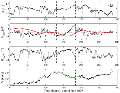
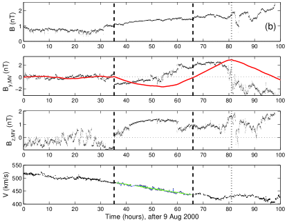
Figure 1: Examples of two MCs with velocity profiles that are not significantly perturbed (i.e. that have an almost linear dependence on time). (a) MC 13 travels at low latitude ($2\degr$) at $D=5.3$ AU in a slow SW and (b) MC 30 travels at high latitude ($-66\degr$) at $D=3$ AU in a relatively slow SW for such high latitude. The vertical dashed lines define the MC (flux rope) boundaries, and the vertical dotted line defines the rear boundary of the MC back (Sect. 2.3, a back is only present on the right panels). The three top panels show the magnetic field norm and its two main components in the MC frame computed with the MV method (Sect. 2.2). $B_{\rm z,MV}$ is the MC axial magnetic field component. $B_{\rm y,MV}$ is the magnetic field component both orthogonal to the MC axis and to the radial direction from the Sun ($\hat{\bf R}$). The solid red line represents $F_{\rm y}$, which is the accumulated flux of $B_{\rm y,MV}$ [Eq. (1)]. The bottom panel shows the observed velocity component in the radial direction ($\hat{\bf R}$). A linear least squares fit of the velocity (green line) is applied in the time interval where an almost linear trend is present within the MC.

2 Data and method

2.1 Selected MCs

We derive the generic expansion properties of MCs in the outer heliosphere. We do not select MCs based on their physical properties (e.g. depending on whether they drive a front shock for instance), but rather study a set, as complete as possible, of MCs in a given period of time. We select the MCs previously analyzed by Rodriguez et al. (2004) based on their thermal and energetic properties. This list of 40 MCs covers the time interval from February 1992 to August 2002. During the analysis of Ulysses data, we find six extra MCs during this time interval, which are included at the end of Table 3.

Our present study has a different scope from Rodriguez et al. (2004) as our main aim is to quantify the expansion properties of MCs. We use data from the Solar Wind Observations Over the Poles of the Sun (SWOOPS, Bame et al., 1992) of plasma observations with a temporal cadence of 4 minutes. The magnetic field data are from the Vector Helium Magnetometer (VHM, Balogh et al., 1992), and have a temporal cadence of one second.

2.2 The MC frame

The magnetic and velocity fields observations are in the radial tangential normal (RTN) system of reference ($\hat{\bf R}$, $\hat{\bf T}$, $\hat{\bf N}$), where $\hat{\bf R}$ points from the Sun to the spacecraft, $\hat{\bf T}$ is the cross product of the Sun’s rotation vector with $\hat{\bf R}$, and $\hat{\bf N}$ completes the right-handed system (e.g., Fränz & Harper, 2002).

Another very useful system of coordinates is one attached to the local direction of the flux rope. In this MC local frame, $\hat{\bf Z}_{\rm cloud}$ is aligned along the cloud axis (with $B_{z,\rm cloud}>0$ in the MC central part), and found by applying the minimum variance (MV) technique to the normalized time series of the observed magnetic field (e.g. Gulisano et al., 2007, and references therein). We define $\hat{\bf Y}_{\rm cloud}$ in the direction $\hat{\bf R}\times\hat{\bf Z}_{\rm cloud}$, and $\hat{\bf X}_{\rm cloud}$ completes the right-handed orthonormal base ($\hat{\bf X}_{\rm cloud},\hat{\bf Y}_{\rm cloud},\hat{\bf Z}_{\rm cloud}$).

In the MC frame, the magnetic field components have a typical behavior that we now describe. The axial field component, $B_{z,\rm cloud}$, typically reaches a maximum in the central part of the MC, and declines toward the borders to small, or even negative, values. The component $B_{y,\rm cloud}$ typically changes of sign in the MC central part. When large fluctuations are present in some MCs, then $B_{y,\rm cloud}$ has an odd number of reversals (e.g. Steed et al., 2011). Finally, the component $B_{x,\rm cloud}$ has its weakest value when the spacecraft crosses the central part of the MC; its relative magnitude provides an indication of the impact parameter (Gulisano et al., 2007; Démoulin & Dasso, 2009b).

Another reason for being interested in the MC frame is that it permits us to relate the inward and outward limits of the crossed flux rope to the conservation of the azimuthal flux (Dasso et al., 2006). We neglect the evolution of the magnetic field during the spacecraft crossing period (since the elapsed time is small compared to the transit time from the Sun, see Démoulin et al., 2008 for a justification), and define the accumulative flux per unit length $L$ along the MC axial direction as (Dasso et al., 2007)

$$\frac{F_{y}(t)}{L}=\int_{t_{\rm in}}^{t}B_{y,cloud}(t^{\prime})\leavevmode\nobreak\ V_{x,cloud}(t^{\prime})\leavevmode\nobreak\ {\mathrm{d}}t^{\prime}\,,$$ (1)

where $t_{\rm in}$ is the time of the front boundary. This time is selected as a reference since the front boundary is usually well-defined, although any other reference time can be used without any effect on the following conclusions. Since $B_{y,cloud}$ undergoes its principal change of sign inside a MC, $F_{y}(t)$, then has a main extremum and defines the time called $t_{\rm center}$, which is approximately the time of closest approach to the flux rope center. With the hypothesis of a local symmetry of translation along the main axis, the flux surface passing at the position of the spacecraft at time $t_{1}$ is wrapped around the flux rope axis, and is observed at time $t_{2}$ defined by

$$F_{y}(t_{1})=F_{y}(t_{2})\,,$$ (2)

from the conservation of the azimuthal flux. Within the flux rope, this equation relates any inward time (time period for inward motion) to its conjugate in the outward (the same but for outward motion).

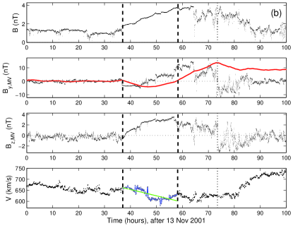
Figure 2: Examples of two MCs with perturbed velocity (i.e. deviating from a linear function of time). (a) MC 11 travels at low latitude ($6\degr$) at $D=5.2$ AU in a slow SW and (b) MC 36 travels at high latitude ($75\degr$) at $D=2.3$ AU in a fast SW. We use the same quantities and drawing convention as Fig. 1.

2.3 Definition of the MC boundaries

As a first approximation, we choose the MC boundaries from the magnetic field in the RTN coordinate system, taking into account the magnetic field properties (see Section 1). We also consider the measured proton temperature and compared them to the expected temperature in the SW with the same speed (Lopez & Freeman, 1986) and to SW temperature accounting for its dependence on solar distance (Wang et al., 2005b). However, a lower temperature than expected is only used as a guide, since we found that the magnetic field has sharper changes than the temperature (observed in the time series of data), and so the magnetic field defines more precisely the flux rope boundaries.

The front, or inward, boundary of a MC is typically the easiest to determine. It is the limit between the fluctuating magnetic field of the sheath and the smoother field variation within the flux rope. A current sheet is typically present between these two regions, and the front boundary is defined to be there, at a time denoted $t_{\rm in}$.

The rear, or outward, boundary is more difficult to define, particularly because many MCs have a back region with physical properties that are in-between those of the MC and SW hence the transition between the flux rope and the perturbed SW is frequently not as well defined as at the inward boundary. Dasso et al. (2006, 2007) concluded that this back region is formed, during the transit from the Sun, by reconnection of the flux rope with the overtaken magnetic field. We use the conservation of the azimuthal flux between the inward and outward boundary, Eq. (2), to define the outward boundary. When a back region is present, the time $t_{\rm out}$ of the outward boundary is defined as the first solution of $F_{y}(t_{\rm out})=F_{y}(t_{\rm in})=0$. However, this condition depends on the determination of the MC frame thus an iterative procedure is needed, as follows.

We start with approximate MC boundaries defined in the RTN system, then perform a MV analysis to find the local frame of the MC. Next, we analyze the magnetic field components in the local frame, and redefine the boundaries according to the azimuthal flux conservation expected in a flux rope [Eq. (2)]. In most cases, the temporal variations in the magnetic components indicate that the rear boundary needs to be change its location. The MV analysis is then performed only on the flux rope interval. This is an important step because an excess of magnetic flux on one side of the flux rope typically introduces a systematic bias in the MV directions. Finally, we perform the same procedure iteratively until convergence is achieved. This defines more reliably determined boundaries and orientation of the flux rope.

As at the front boundary, we expect to find a current sheet at the outward boundary (since it separates two regions with different origins and physical properties). A current sheet is typically found at about time $t_{\rm out}$ in most analyzed MCs . The bending of the flux rope axis is one plausible cause of the small difference in time between $t_{\rm out}$ and the closest current sheet.

In the outward branch of a few MCs, $B_{y,\rm cloud}$ has an important current sheet and later on it fluctuates before $F_{y}(t)$ finally vanishes. This indicates that there is a deficit of azimuthal flux in the outward branch compared to the inward one. In this case, $t_{\rm out}$ is defined by the observed time of the current sheet, and the flux rope extension is in the time interval $[t_{\rm in},t_{\rm out}]$, where $t_{\rm in}$ is redefined by $F_{y}(t_{\rm in})=F_{y}(t_{\rm out})$. The iterative procedure described above is then applied to improve $t_{\rm in}$ and the flux rope orientation.

2.4 MC groups

Following Gulisano et al. (2010), we divide the data set into three groups: non-perturbed MCs, perturbed MCs, and MCs in interaction (noted interacting).

The interacting group contains the MCs that have a strong magnetic field nearby (e.g. another MC). From MHD simulations, their physical properties are expected to differ significantly from non-interacting MCs (e.g., Xiong et al., 2007). Observations, indeed confirm that MCs in the process of interacting could have a different behavior from non-interacting MCs (e.g. Wang et al., 2005a; Dasso et al., 2009).

The MCs in the non-perturbed and perturbed groups have less disturbed surroundings than MCs in the interacting group. The MCs in the non-perturbed group have an almost linear velocity profile in more than $75$% of the flux rope, while in the perturbed MCs this condition is not satisfied. Two examples of each group are shown in Figs. 1,2, the label (number), the group, and the main properties of each MC are given in Table 3.

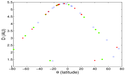
Figure 3: Spatial localization of the MCs listed in Table 3. The MCs are separated into three groups: non-perturbed (filled green circles), perturbed (empty blue squares), and in the process of interaction (red stars).

Table 1: Exponents $e$ in the fit with a power law $D^{e}$ for $S$, $<B>$, and $<N_{\rm p}>$ (found by performing a linear fit in log-log plots, Fig. 4).

range of $D$ a	$S$ b		$<B>$ b		$<N_{\rm p}>$ b		Ref.c
all MCs
$[1.4,5.4]$	$0.49$	$\pm 0.26$	$-1.20$	$\pm 0.20$	$-1.70$	$\pm 0.34$	c
non-perturbed and
perturbed MCs
$[0.3,1]$	$0.78$	$\pm 0.12$	$-1.85$	$\pm 0.07$			c
$[1.4,5.4]$	$0.56$	$\pm 0.34$	$-1.18$	$\pm 0.27$	$-1.70$	$\pm 0.43$	c
non-perturbed MCs
$[0.3,1]$	$0.89$	$\pm 0.15$	$-1.85$	$\pm 0.11$			c
$[1.4,5.4]$	$0.79$	$\pm 0.46$	$-1.39$	$\pm 0.92$	$-2.24$	$\pm 0.66$	c
perturbed MCs
$[0.3,1]$	$0.45$	$\pm 0.16$	$-1.89$	$\pm 0.10$			c
$[1.4,5.4]$	$0.54$	$\pm 0.48$	$-1.14$	$\pm 0.26$	$-1.40$	$\pm 0.50$	c
MCs
$[0.3,1]$					$-2.40$	$\pm 0.30$	c
$[0.3,1]$	$1.14$	$\pm 0.44$	$-1.64$	$\pm 0.40$	$-2.44$	$\pm 0.46$	c
$[0.3,4.]$	$0.97$	$\pm 0.10$	$-1.80$		$-2.8$		c
$[0.3,4.8]$	$0.78$	$\pm 0.10$					c
$[0.3,5.4]$	$0.61$	$\pm 0.09$	$-1.30$	$\pm 0.09$	$-2.62$	$\pm 0.07$	c
$[1.4,5.4]$			$-0.88$	$\pm 0.22$			c
ICMEs
$[0.3,5.4]$	$0.61$		$-1.52$				c
$[0.3,5.4]$	$0.92$	$\pm 0.07$	$-1.40$	$\pm 0.08$	$-2.32$	$\pm 0.07$	c

• The range of solar distances is in astronomical units (AU). In the middle part of the table, MCs are separated in non-perturbed and perturbed MCs.

• The exponents, $e$, are given for the size $S$ in the $\hat{\bf R}$ direction, the mean magnetic field strength $<B>$, and the mean proton density $<N_{\rm p}>$. All quantities are computed within the flux rope boundaries.

• We compare our results with our previous results in the inner heliosphere and with other studies of MCs and ICMEs. The results are from: ^c: present work, ^c: Gulisano et al. (2010), ^c: Bothmer & Schwenn (1998), ^c: Leitner et al. (2007), ^c: Kumar & Rust (1996), ^c: Wang et al. (2005b), ^c: Liu et al. (2005).

3 Magnetic cloud size and mean properties

We now analyze the size and mean properties, along the spacecraft trajectory, of MCs as a function of solar distance $D$. Because of the trajectory of Ulysses, a correlation between $D$ and the absolute value of the latitude is present in the analyzed data (Fig. 3). However, the results of the analysis that we now describe do not change significantly when MCs are grouped in terms of the latitude, so that this correlation between $D$ and latitude does not affect our conclusions. All the studied properties are affected by the expansion achieved from the Sun to Ulysses. From models (see e.g., Chen, 1996; Kumar & Rust, 1996; Démoulin & Dasso, 2009a), all properties are expected to have a power-law dependence on $D$, we then perform a linear fit for each property plotted on a log-log scale (Figs. 4,5), for the non-perturbed and perturbed groups. Since MCs in interaction are strongly case-dependent, their properties are not compared (fitted) with the global models here.

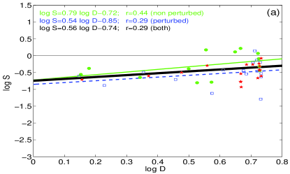
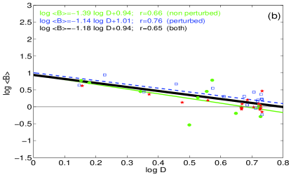
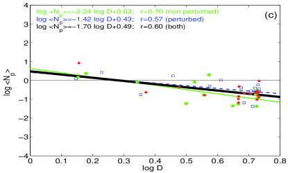
Figure 4: Dependence on the solar distance, $D$ in AU, of (a) the radial size in the $\hat{\bf R}$ direction (AU), (b) the mean magnetic field strength (nT), and (c) the mean proton density (cm^-3) with log-log plots. The MCs are separated in three groups: non-perturbed (filled green circles), perturbed (empty blue squares), and in interaction (red stars). The straight lines are the result of a least squares fit for non-perturbed (thin continuous green line), perturbed (dashed blue line), and for non-perturbed and perturbed MCs (thick continuous black line). The fits and the absolute value of the correlation coefficients, r, are added at the top of each panel.

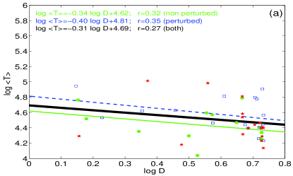
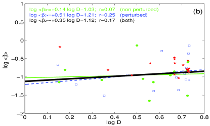
Figure 5: Dependence on the solar distance, $D$ in AU, of (a) the mean proton temperature $<T_{p}>$ (K) and (b) the mean proton $\beta$. The drawing convention is the same than in Fig. 4.

3.1 Magnetic cloud size

With the MC boundaries defined in Sect. 2.3, we compute the size $S$ in the direction $\hat{\bf R}$ as the product of the duration of the MC and its velocity at closest approach to the center of the flux rope. Compared to most previous works (see Sect. 1), this typically defines a smaller size as the back region is not included.

Since the majority of previous studies include all MCs independently of the groups we defined above, we first compare them to our results with all MCs included (Table 1). In the range [1.4,5.4] AU, we find an exponent that is lower ($0.49\pm 0.26$) than previous studies on MCs or ICMEs in the inner and outer heliosphere (lower part of Table 1). Taking into account only non-perturbed and perturbed MCs, the exponent is slightly higher ($0.56\pm 0.34$), but still lower than previous studies, including our previous result obtained with Helios data ($0.78\pm 0.12$).

Next, we analyze separately the non-perturbed and perturbed MCs. In the range [1.4,5.4] AU, we find comparable exponents to our previous results obtained with Helios data for both non-perturbed and perturbed MCs (Table 1). Perturbed MCs have a significantly smaller size on average than non-perturbed MCs and this tendency increases with solar distance (Fig. 4a). We find that perturbed MCs typically have smaller sizes $S$, by a factor $\approx 1.3$, than non-perturbed MCs.

The MCs in interaction (interacting MCs) have typically smaller sizes $S$ than the non-perturbed MCs (Fig. 4a). We interpret this result as a direct effect of the compression and/or reconnection with the interacting MC or strong magnetic-field structure.

3.2 Magnetic field strength

We define the average field $<B>$ within the flux rope boundaries defined in Sect. 2.3 and proceed as above with $S$. The value of $<B>$ decreases far more slowly with distance in the Ulysses range ($-1.18\pm 0.27$) than the Helios range ($-1.85\pm 0.07$) for the non-perturbed and perturbed MCs (a similar result is obtained when also including the interacting MCs). Finally, combining our Helios and Ulysses results, we have an intermediate exponent ($-1.5\pm 0.1$). This last result is closer to the results of Wang et al. (2005b) and Liu et al. (2005) obtained for a larger set of ICMEs across the same range of distances (bottom of Table 1).

The non-perturbed MCs have a slightly steeper decrease in magnetic field strength with distance than the perturbed MCs (Fig. 4b). This result is coherent with the conservation of magnetic flux combined with a slightly larger increase in size with distance of the non-perturbed MCs compared to the perturbed ones. We also find that the perturbed MCs typically have a stronger magnetic field, by a factor of between $\approx 1.4$ and $1.7$, than non-perturbed MCs (Fig. 4b), a result that is consistent with the lower expansion rate for perturbed MCs (see Sect. 3.1 and 4.3).

The interaction has a weaker effect on $<B>$ than on the size $S$: There is only a weak tendency for interacting MCs to have stronger $<B>$ than non-perturbed MCs (Fig. 4b).

Table 2: Average and dispersion in the main parameters of MCs from our present study and Du et al. (2010).

Group a	$V_{c}$ b	$S_{\rm 1\,AU}$ c	$<B>_{\rm 1\,AU}$ c	$<N_{\rm p}>_{\rm 1\,AU}$ c	$<\beta_{p}>$	$\gamma$ d	$\zeta$ e
	km/s	AU	nT	cm-3		°
all MCs	470$\pm$110	0.16$\pm$0.12	12$\pm$7	9$\pm$8	0.19$\pm$0.17	68$\pm$17	0.77$\pm$0.75
non-perturbed and perturbed	480$\pm$120	0.18$\pm$0.14	14$\pm$8	9$\pm$8	0.18$\pm$0.19	68$\pm$20	0.63$\pm$0.59
non-perturbed	480$\pm$130	0.24$\pm$0.16	11$\pm$9	7$\pm$10	0.17$\pm$0.18	63$\pm$24	1.05$\pm$0.34
perturbed	480$\pm$110	0.13$\pm$0.09	16$\pm$6	11$\pm$7	0.19$\pm$0.20	72$\pm$15	0.28$\pm$0.52
interacting	470$\pm$130	0.12$\pm$0.05	10$\pm$6	9$\pm$9	0.22$\pm$0.14	66$\pm$13	1.00$\pm$0.93
MCf	500$\pm$100	0.26$\pm$0.19	11$\pm$6				0.59$\pm$0.51
non-MC ICMEf	480$\pm$ 90	0.22$\pm$0.21	5$\pm$4				0.68$\pm$0.48

• The MCs are separated into three groups: non-perturbed, perturbed, and interacting.

• The size and the mean field are normalized to 1 AU according to Eq. (8) and the proton density with $<N_{\rm p}>_{\rm 1\,AU}=<N_{\rm p}>D^{2.2}$, where $D$ is the solar distance in AU.

• $\gamma$ is the angle between the MC axis and the radial direction ($\hat{\bf R}$).

• $\zeta$ is the nondimensional expansion rate [Eq. (5)].

• Computed from the results of Du et al. (2010).

3.3 Proton density

We define the average proton density $<N_{\rm p}>$ as above for the magnetic field strength, i.e. within the flux rope boundaries. For the non-perturbed and perturbed MCs, the density decreases significantly less rapidly with distance (exponent $=-1.70\pm 0.43$) than in previous studies (exponents in the range $[-2.8,-2.3]$) for both the inner heliosphere and a combination of both the inner and outer heliosphere. However, we are unaware of results for the outer heliosphere alone (apart Fig. 10 of Leitner et al., 2007, but no fit is provided).

Nevertheless, for the non-perturbed MCs the density decreases with $D$ following a powerlaw that is in closer agreement with previous studies. In contrast, for perturbed MCs the density decreases much more slowly with distance. This agrees qualitatively with a lower expansion of $S$ and a lower decrease in $<B>$ with $D$, while the difference between non-perturbed and perturbed MCs is more significant for the average proton density. Even if there is qualitative agreement, the systematically smaller decrease in $<N_{\rm p}>$ with $D$ than in previous studies could be related to the substantial variability of $N_{\rm p}$ in MCs (e.g. at 1 AU see Lepping et al., 2003) so that $<N_{\rm p}>$ is case dependent and could be biased with our relatively small number of MCs. When the same MC is observed at two distances, this bias is removed. For MC 15, we computed from the observed data a steeper slope of $2.9$ by using the mean observed density at both ACE and Ulysses (Nakwacki et al., 2011).

The effect of the interaction on $<N_{\rm p}>$ is weak, and comparable to the effect on $<B>$: there is only a weak tendency for interacting MCs to have stronger $<N_{\rm p}>$ than non-perturbed MCs (Fig. 4c). While there are too few interacting MCs at low $D$ to enable us to draw a strong conclusion, the trend of a global decrease in $<N_{\rm p}>$ with $D$ predominates over the effect (typically compression) of an interaction with another MC or a strong B region.

3.4 Proton temperature

The average proton temperature decreases only weakly with distance (Fig. 5a). The temperatures of the non-perturbed and perturbed MCs have dependences close to $D^{-0.34}$ and $D^{-0.40}$, respectively. This contrasts with the decrease found in the SW, which is typically around $D^{-0.7}$ (Gazis et al., 2006; Richardson & Cane, 1995). Moreover, the interacting MCs are not significantly hotter than non-perturbed and perturbed MCs (apart from two hot interacting MCs, Fig. 5a).

The above result also differs from the decrease in temperature given by $\approx D^{-1.6}$ found by Leitner et al. (2007) for MCs observed in the range $[0.3,5.4]$ AU. However, our results agree with those of Leitner et al. (2007) since their Fig. 11 shows no decrease in proton temperature with distance for MCs observed by Ulysses. We conclude, in agreement with previous results, that the proton temperature of MCs in the outer heliosphere decreases with $D$ much more slowly than in the inner heliosphere and than in the SW.

Moreover, MCs have a much larger volume expansion than the SW, the main difference being that MCs have a significant expansion in the radial direction (Table 1 and Fig. 6 below) in contrast to the SW, which has no mean radial expansion. Considering an adiabatic expansion implies that MCs should become even cooler than the SW with distance. The opposite is in fact observed, which implies that there is a far greater amount of heating in the MCs than the SW. A significant source of this heating could be a turbulent cascade to small scales. Since $\beta_{\rm p}<<1$ in MCs (see Sect. 3.5), the dissipation of a small fraction of the magnetic energy provides a large increase in the plasma temperature, while the same amount of magnetic energy in the SW provides only a small increase in the plasma temperature ($\beta_{\rm p}\approx 1$).

3.5 Proton plasma $\beta$

The proton plasma $\beta$, denoted $\beta_{\rm p}$, is defined as the ratio of the proton thermal pressure to the magnetic pressure. Thus, if the decay of the proton density, proton temperature, and magnetic field intensity are true power laws (respectively, $N_{p}\propto D^{-n_{n}}$, $T_{p}\propto D^{-n_{T}}$, and $B\propto D^{-n_{B}}$), the decay of $\beta_{\rm p}$ will be $\beta_{\rm p}\propto D^{-n_{n}-n_{T}+2n_{B}}$, which in our Ulysses study corresponds to an expected increasing function with the heliodistance, such as $\beta_{p,exp}\propto D^{-1.7-0.31+2*1.18}\sim D^{+0.35}$ for the combined sample of non-perturbed and perturbed MCs (Figs. 4b,c, 5a). Another estimation can be realized by supposing an isotropic expansion of MCs with distances that increase as $D^{m}$. Assuming the conservations of both mass and magnetic flux (i.e., an ideal regime), we theoretically expect an evolution such that $\beta_{\rm p}\propto D^{-3m-n_{T}+4m}$, which is $\beta_{\rm p}\propto D^{+0.25}$ for non-perturbed and perturbed MCs and $\beta_{\rm p}\propto D^{+0.45}$ for non-perturbed MCs, and then comparable to the previous estimation.

We compute the mean value of $\beta_{\rm p}$ within each studied cloud, finding that $<\beta_{\rm p}>$ is lower than unity for all MCs in our sample, and has a tendency to slightly increase with solar distance for non-perturbed and perturbed MCs. We find that $\beta_{\rm p}\propto D^{0.35}$ for the combined groups of MCs (Fig. 5b), so a very similar dependence to that found above assuming exact power laws.

Leitner et al. (2007) found a slight decrease, $\approx D^{-0.4}$, for MCs in the range $[0.3,5.4]$ AU. However, this global tendency is not present for MCs observed with Ulysses, as their Fig. 12 shows a tendency of increasing $\beta_{\rm p}$ with $D$. We then conclude that $\beta_{\rm p}$ has a different dependence on $D$ in both the inner and outer heliosphere.

Next, we analyze separately the dependence of $\beta_{\rm p}$ on $D$ for each MC group. The value of $\beta_{\rm p}$ is almost independent of $D$ for the non-perturbed MCs, and the above increasing trend with distance can be mainly attributed to the perturbed MCs. The MCs that are interacting typically have a larger $\beta_{\rm p}$ at all $D$ (Fig. 5b).

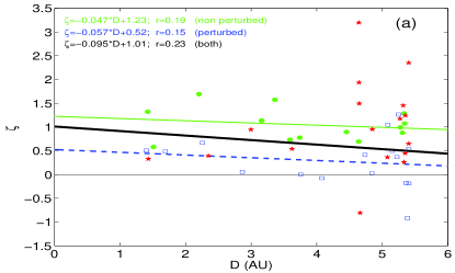
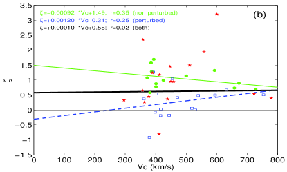
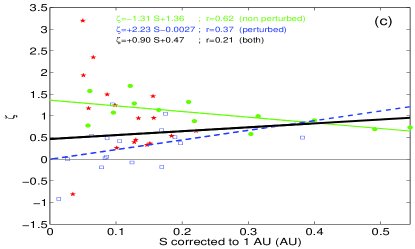
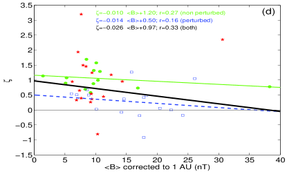
Figure 6: The panels (a-d) show the correlation analysis that tests for the dependence of the non-dimensional expansion factor $\zeta$ [Eq. (5)] on other MC parameters. The drawing convention is the same as in Fig. 4. Both $S_{\rm 1\,AU}$ and $<B>_{\rm 1\,AU}$ are normalized to 1 AU using the size and field strength dependence on the distance, according to the relationship given in Figure 4 for non-perturbed MCs, see Eq. (8).

4 Expansion rate of MCs

Magnetic clouds typically have a velocity profile close to a linear function of time with a larger velocity in the front than at the rear. Hence MCs are expanding magnetic structures as they move away from the Sun. In this section, we characterize their expansion rate.

4.1 Non-dimensional expansion rate

The measured temporal profile $V_{R}(t)$ of each MC is fitted using a least squares fit with a linear function of time

$$V_{R,\rm fit}(t)=V_{\rm o,fit}+({\mathrm{d}}V_{R}/{\mathrm{d}}t)_{\rm fit}\leavevmode\nobreak\ t\,,$$ (3)

where $({\mathrm{d}}V_{R}/{\mathrm{d}}t)_{\rm fit}$ is the fitted slope. We always keep the fitting range within the flux rope, and restricts it to the most linear part of the observed profile. The observed linear profile of $V_{R}$ indicates that different parts of the flux rope expand at about the same rate in the direction $\hat{\bf R}$.

The linear fit is used to define the velocities $V_{R,\rm fit}(t_{in})$ and $V_{R,\rm fit}(t_{out})$ at the flux rope boundaries (Sect. 2.3). We then define the full expansion velocity of a flux rope as

$$\Delta V_{R}=V_{R,\rm fit}(t_{in})-V_{R,\rm fit}(t_{out})\,.$$ (4)

For non-perturbed MCs, $\Delta V_{R}$, is very close to the observed velocity difference $V_{R}(t_{in})-V_{R}(t_{out})$, see e.g. the lower panels of Fig. 1. For perturbed MCs, this procedure minimizes the effects of the perturbations within the flux rope and especially close to the MC boundaries.

Following Démoulin & Dasso (2009a) and Gulisano et al. (2010), we define the non-dimensional expansion rate as

$$\zeta=\frac{\Delta V_{R}}{\Delta t}\frac{D}{V_{c}^{2}}\,$$ (5)

which defines a scaling law for the size $S$ of the flux rope (along $\hat{\bf R}$) with the distance ($D$) from the Sun as $S\propto D^{\zeta}$. This simple interpretation of $\zeta$ is obtained with the following two simplifications which were justified in Démoulin & Dasso (2009a). Firstly, we neglect the aging effect (the front is observed at an earlier time than the rear, so when observed at the front the flux rope is smaller than when it is observed at the rear), and secondly, $\zeta$ is approximately constant during the time interval of the observed flux rope.

While $\zeta$ is a local measurement within the flux rope, it provides a measure of the exponent $m$ of the flux rope size if it follows a power law

$$S=S_{0}\left(\frac{D}{D_{0}}\right)^{m}\,.$$ (6)

taking the temporal derivative of $S$, we find that

$$\frac{{\mathrm{d}}S}{{\mathrm{d}}t}=\Delta V_{R}=\frac{{\mathrm{d}}S}{{\mathrm{d}}D}\frac{{\mathrm{d}}D}{{\mathrm{d}}t}\approx m\frac{S}{D}V_{c}\approx m\frac{\Delta tV_{c}^{2}}{D}\,.$$ (7)

We then find a relation that is equivalent to Eq. (5), so for self-similarly expanding MCs we have $m\approx\zeta$.

4.2 Expansion of non-perturbed MCs

The main driver of MCs expansion was identified by Démoulin & Dasso (2009a) as the rapid decrease in the total SW pressure with solar distance . They followed the force-free evolution away from the Sun of flux ropes with a variety of magnetic field profiles and assuming either ideal MHD or fully resistive relaxation that preserves magnetic helicity. Within this theoretical framework, they demonstrated that a force-free flux rope has an almost self-similar expansion, so a velocity profile is almost linear with time as observed by a spacecraft crossing a MC (e.g. Figs. 1,2). In the case of a total SW pressure behaving as $D^{-n_{P}}$, they also found that the normalized expansion rate is $\zeta\approx n_{P}/4$. These results apply to a progressive evolution of a flux rope in a quiet SW, so the non-perturbed MCs are expected to have the closest properties to these theoretical results.

The mean value of $\zeta$ for non-perturbed MCs, observed in the range $[1.4,5.4]$ AU, is $<\zeta>\approx 1.05\pm 0.34$. This is slightly above the mean values, $\approx 0.80\pm 0.18$ and $\approx 0.91\pm 0.23$, found at 1 AU and in the range $[0.3,1.]$ AU, respectively (Démoulin et al., 2008; Gulisano et al., 2010). This is a small increase compared to the change in $D$, which is a factor in the definition of $\zeta$ [Eq. (5)]. Since $V_{c}$ has no significant dependence on $D$ (Wang et al., 2005b), the increase in $D$ is compensated for mainly by the decrease in $\Delta V_{R}/\Delta t$.

The slightly higher mean $<\zeta>$ in the range $[1.4,5.4]$ AU is mostly due to the higher $\zeta$ values found at smaller $D$ values (Fig. 6a), so in the region that most closely matches that of both previous studies. Owing to the characteristics of the Ulysses orbit, there are indeed only a few observed MCs for $D<3$ AU (Fig. 3) so that the decrease with $D$ in the linear fit of $\zeta$ could be due to the specific properties of the few detected MCs at these lower distances. We also recall that $D$ is strongly correlated with the heliolatitude $|\theta|$, Fig. 3, so that the dependence $\zeta(D)$ shown in Fig. 6a could also be an effect of latitude. Nevertheless, we emphasize that the $<\zeta>$ found here with Ulysses is only slightly higher than the values found previously at smaller distances from the Sun. These differences are small compared to the significantly different SW properties of the slow and fast SWs predominantly present at low and high latitude, respectively.

As in the previous study, we test the possible dependence of $\zeta$ on the MC properties. Both the MC size and field strength depend strongly on $D$ (Fig. 4a,b). We use the fits found for the non-perturbed MCs to remove, on average, the evolution with $D$. Hence we define values at a giving solar distance, here taken at 1 AU, with the relations

$$S_{\rm 1\,AU} = S\leavevmode\nobreak\ D^{-0.79},$$

$$<B>_{\rm 1\,AU} = <B>\leavevmode\nobreak\ D^{+1.39}\,.$$ (8)

The mean MC speed depends only weakly on $D$ in the outer heliosphere (see e.g. Wang et al., 2005b, for a large set of ICMEs, including MCs), hence we use below the measured velocity of the center $V_{\rm c}$.

For non-perturbed MCs we find that $\zeta$ is almost independent of $<B>_{\rm 1\,AU}$ (Fig. 6d), as found in the range $[0.3,1.]$ AU (compared to Fig. 4d of Gulisano et al., 2010). A small difference is that $\zeta$ decreases slightly with $V_{\rm c}$ and $S_{\rm 1\,AU}$ (Fig. 6b,c), while a nearly constant value was found in the range $[0.3,1.]$ AU (compared to Fig. 4b,c of Gulisano et al., 2010). This difference is probably not due to a latitude dependence since the MCs observed at $|\theta|<25\degr$ or $>25\degr$ are evenly distributed in the three plots when we analyze the two groups independently [not shown], hence similar results are obtained. Finally, using alternative exponents in Eq. (8), in the range given in Table 1, induces only slight changes in the linear fits shown in Fig. 6, particularly in the magnitude of the slope.

 

 

 

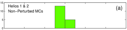
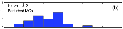
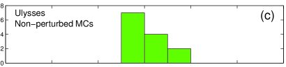
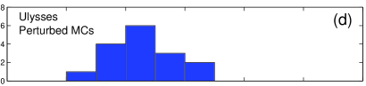
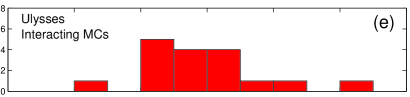
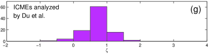
Figure 7: Histograms comparing $\zeta$ of MCs and non-MC ICMEs. (a,b) MCs from Helios spacecraft (Gulisano et al., 2010). (c-e) MCs from Ulysses spacecraft (present work). (f,g) MCs and non-MC ICMEs from Ulysses with approximate $\zeta$ values computed from the results of Du et al. (2010).

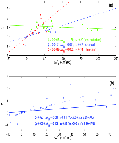
Figure 8: Perturbed and non-perturbed MCs have a remarkably different behavior of $\zeta$ when they are plotted as a function of $\Delta V_{R}$. The drawing convention is the same as that in Fig. 4 for panel (a), while the perturbed MCs are grouped in terms of velocity and distance in panel (b), as indicated by the legend.

4.3 Expansion of perturbed MCs

The main difference between perturbed and non-perturbed MCs, is that the former has a lower expansion rate and a larger dispersion, $<\zeta>=0.28\pm 0.52$, compared to $<\zeta>=1.05\pm 0.34$ for non-perturbed MCs (see also Fig. 7c,d). These results are comparable to the results found in the distance range $[0.3,1]$ AU by Gulisano et al. (2010) since they found $<\zeta>=0.48\pm 0.79$ and $<\zeta>=0.91\pm 0.23$ for perturbed and non-perturbed MCs, respectively (Fig. 7a,b). This lower expansion rate for perturbed MCs is indeed expected from MHD simulations if the origin of the perturbation is an overtaking magnetized plasma, which compresses the MC, hence decreases its expansion rate (Xiong et al., 2006a, b).

A substantial overtaking flow, with a velocity larger than at the front of the MC, is found in 12 of the 20 perturbed MCs. These strong flows are located behind the observed MC, and typically a shock, or at least a rapid variation in $V$, is present at the rear boundary of the back region, as illustrated by MC 11 in Fig. 2a. This is the main difference from MCs observed in the range $[0.3,1]$ AU, as the overtaking flow typically entered deeply into the perturbed MCs, and moreover, a strong shock was typically present within the perturbed MC (compare Fig. 2a with Fig. 2 Gulisano et al., 2010). This difference can be interpreted with the MHD simulations of Xiong et al. (2006a, b), as follows. The observations at Helios distances correspond to the interacting stage when the overtaking shock travels inside the MC (e.g. see Fig. 5 of Xiong et al., 2006a). At larger solar distances, the overtaking shock exits from the front of the MC, hence it is not observed inside the MC with Ulysses data. However, some of the overtaking flow is present behind the MC. The compression of the overtaking flow thus persists, and most perturbed MCs are under-expanding.

Additional evidence of a different evolution stage at Ulysses compared with Helios is that $\zeta$ shows no significant dependence on $D$ (Fig. 6a), while the mean tendency of $\zeta$ was to increase with $D$ and to reach the value of $<\zeta>$ at 1 AU of unperturbed MCs for Helios MCs (Fig. 4a Gulisano et al., 2010).

Only one perturbed MC expands slightly faster than the mean expansion rate of unperturbed MCs (Fig. 6), while a stronger over-expansion is present in some MCs in interaction. These, over-expanding flux ropes can be identified in the above MHD simulations in the late stage of evolution, as follows. The overtaking magnetized plasma progressively flows on the MC sides and overtakes the MC. When only a weak overtaking flow remains at the MC rear, the expansion rate could increase. The MC internal magnetic pressure is indeed higher (owing to the previously applied compression) than the pressure value for another MC at the same position and with no overtaking flow before. This over-pressure drives a more rapid MC expansion (e.g. see the summary of two simulations in Fig. 7 of Xiong et al., 2006a). Hence, the expansion rate of perturbed MCs depends on the interaction stage in which they are observed, (see the cartoon in Figure 6 of Gulisano et al., 2010).

Some properties of $\zeta$ for perturbed MCs are still similar in the inner and outer heliosphere. The value of $\zeta$ shows an increase with both $V_{\rm c}$ and $S_{\rm 1\,AU}$ (Fig. 6b,c), and a decrease with $<B>_{\rm 1\,AU}$ (Fig. 6d) as found with Helios data (Fig. 4b,c,d Gulisano et al., 2010). However, the slope values are smaller by a factor $\approx 2.2$, and $6$, respectively. Finally, we note that the above differences are not due to a difference in the range of parameters since $V_{\rm c}$, $S_{\rm 1\,AU}$, and $<B>_{\rm 1\,AU}$ have similar ranges for Helios and Ulysses MCs.

As for Helios MCs, $\zeta$ does not depend on the expansion velocity $\Delta V_{R}$ [defined by Eq. (4)] for non-perturbed MCs observed by Ulysses, while $\zeta$ is strongly correlated with $\Delta V_{R}$ for perturbed MCs (compare Fig. 8a with Fig. 5 in Gulisano et al., 2010). This result extends previous Helios results to large distances. Non-perturbed MCs indeed have an intrinsic expansion rate $\zeta$ (which is given by the decrease in the total SW pressure with solar distance). This is not the case for perturbed MCs, which are in a transient stage, so $\Delta V_{R}$ cannot be computed by ${\mathrm{d}}S/{\mathrm{d}}t$ as done in Eq. (7). Following the derivation of Gulisano et al. (2010), we instead find that

$$\zeta_{\rm perturbed}=\frac{\Delta V_{R}}{S}\frac{D}{V_{c}}\approx\frac{\Delta V_{R}D_{0}^{m}D^{1-m}}{S_{0}V_{c}}\,,$$ (9)

where the MC size $S_{0}$ is taken at distance $D_{0}$. For perturbed MCs, one then expects that $\zeta$ is linearly dependent on $\Delta V_{R}$, which is indeed true (Fig. 8a). Interacting MCs are strongly perturbed, and indeed $\zeta$ depends more strongly on $\Delta V_{R}$ than the group we call perturbed.

Moreover, from Eq. (9), a dependence of $\zeta$ on both $D$ and $V_{c}$ is expected. Within the observed ranges, both parameters have a comparable effect on the slope. Since we have a too small number of MCs to perform a test to assess the dependence on both $D$ and $V_{c}$, we only considered the two groups where $D$ and $V_{c}$ appear to have a combined effect on the slopes. Hence, these two groups have larger slope differences, and luckily, are also the most numerous groups. The first group is defined by $V_{c}<500$ km/s and $D>4$ AU, or more precisely $<V_{c}>\approx 410$ km/s and $<D>\approx 5.1$ AU. The second group is defined by $V_{c}>500$ km/s and $D<4$ AU, or more precisely $<V_{c}>\approx 640$ km/s and $<D>\approx 2.6$ AU. We use a typical $S_{0}=0.2$ AU value at $D_{0}=1$ AU, and $m=0.54$ as found for perturbed MCs (Table 1). The first group has an expected slope of $0.026$, which is comparable to the one derived from the data ($0.028$, Fig. 8b). The second group is expected to have a smaller slope value of $0.012$ and the observations do indeed give a slope that is even lower by a factor $1.5$. One can also compare the ratio of predicted to observed slopes to eliminate the influence of $S_{0}$: the observed ratio of slopes is a factor $1.6$ larger than the predicted one, and decreases to $1.4$ if we use $m=0.28$, the mean $\zeta$ value found for perturbed MCs (Table 2). Taken into account the uncertainties in the MC parameters, these results indeed show that Eq. (9) illustrates that there is a quantitative dependence of $\zeta$ on both $D$ and $V_{c}$ for perturbed MCs.

4.4 Global radial expansion

The determination of $\zeta$ provides the expansion rate of the MC at the time of the observations, while its size $S$ depends on the past history of $\zeta$. If $S$ were observed at another solar distance, this would provide global information on the expansion between the two distances (as well as another piece of local information about $\zeta$). However, the observation of the same MC by two spacecraft is a rare event since it requires a close alignment of the spacecraft positions with the propagation direction of the MC (one case was analyzed by Nakwacki et al., 2011). Nevertheless, the statistical evolution of $S$ with $D$ provides a constraint on the mean evolution of MCs. The flux rope size of non-perturbed MCs have a mean dependence close to (Fig. 4a)

$$S\propto D^{0.79\pm 0.46}\,.$$ (10)

If a MC evolves while $\zeta$ remains constant, this implies that $S\propto D^{\zeta}$ (Sect. 4.1). The non-perturbed MCs are expected to have the most stable $\zeta$ value. Their mean $\zeta$ value, $1.05\pm 0.34$ (Table 2), indicates that they are undergoing a more rapid expansion than indicated by the global results of Eq. (10). The possible difference is that the flux rope size decreases with distance owing to a reconnection with the encountered SW magnetic field. The evidence of this reconnection is a back region observed in a large number of MCs (e.g. a back region is present in the three MCs shown in Figs. 1,2). If the flux rope size were to decrease by a factor $\approx 1.5$ between $1.4$ and $5.4$ following a power law of $D$, it would decrease $S$ by $D^{0.3}$, so sufficiently to explain the above difference between the mean evolution of $S$ [Eq. (10)] and $<\zeta>$ for non-perturbed MCs.

An alternative possibility is that, at least, some of the non-perturbed MCs were in fact previously perturbed so that their $\zeta$ value was lower. This would be indicative of a lower global expansion of the MC, hence a weaker dependence of $S$ on $D$. We indeed find that $<\zeta>=0.77\pm 0.75$ for non-perturbed, perturbed, and interacting MCs taken together, which is much closer to the exponent in Eq. (10) than $<\zeta>$ for the unperturbed MCs alone. According to this view, the unperturbed, interacting, and perturbed classifications are local ones, which are only valid around the time of the observation, and a MC changes its group (non-perturbed/perturbed/interacting) as it travels away from the Sun. Finally, both of the aforementioned possibilities could be happening.

4.5 Magnetic cloud and ICME expansion

We now analyze a broader set of MCs and ICMEs from the results published by Du et al. (2010). They defined ICMEs following Wang et al. (2005b) as the time intervals where the proton temperature, $T_{p}$, was less than half the expected temperature in the SW with the same speed when measured in Kelvin degrees. They found that about 43% of the identified ICMEs are MCs. Their Ulysses data set covers the time interval from January 1991 to February 2008. The mean values of the principal parameters of this data set are given in Table 2. Both groups have similar characteristics to the MCs studied in this paper, with the exception of a significantly lower magnetic-field strength in non-MC ICMEs.

Du et al. (2010) performed a linear fit to the radial velocity through the full ICME (defined by $T_{p}$, while we restrict ourselves to the interior of the flux rope in our study). They defined $\Delta V$ as the speed difference between the leading and trailing edges of the ICME. The distribution of $\Delta V$ is quite similar for MCs and non-MC ICMEs (Du et al., 2010, Fig. 4). The main differences are merely that few MCs have a large $\Delta V$ and that more non-MC ICMEs have very small $\Delta V$.

In their table of ICMEs, Du et al. (2010) provided all the quantities to compute $\zeta$ [Eq. (5)]. We find Gaussian-shaped histograms of $\zeta$ for both MCs and non-MC ICMEs (Fig. 7f,g). They are very similar; in particular, their means and dispersions are comparable ($\zeta=0.59\pm 0.51$ for MCs and $\zeta=0.68\pm 0.48$ for non-MC ICMEs). This is compatible with a common idea that non-MC ICMEs have the same properties as MCs, but are simply observed in situ near their periphery in such a way that the internal flux rope is missed.

These results are also comparable to our results when we group all MCs together, particularly when we consider non-perturbed and perturbed MCs (Fig. 7, Table 2). However, our detailed analysis permits us to distinguish MCs that are in different conditions. The MCs in interaction have a broader range of $\zeta$ (Fig. 7e) since they are strongly affected by the interaction, and they are observed at different times of the interaction process. The non-perturbed MCs logically have the smallest dispersion in $\zeta$ (Fig. 7c). Hence, in addition to the dispersion in $\zeta$ found from the Du et al. (2010) results, we find that different environments or/and evolution stages are present.

5 Magnetic clouds in interaction

5.1 Evolution of MCs in a complex solar wind

Some MCs travel in a structured SW formed by plasma coming from different parts of the solar corona. These plasmas have different properties, for instance in terms of plasma speed and magnetic field, so they are interacting. For example, a rarefaction region is formed when a fast SW precedes a slow SW, while a compression region is formed when a fast SW overtakes a slow SW. Moreover, especially around the maximum of the solar cycle, several ICMEs could be ejected from the Sun at similar times, then interact later on. When a MC travels through a structured SW, the encountered structures affect its evolution.

The group of perturbed MCs, analyzed above, are interpreted as examples of MCs affected during their travel from the Sun by the encountered SW structures. However, since the analyzed data mostly correspond to events that have interacted in the past, there is no direct evidence of the interaction in the in situ data. The previous interactions of these MCs can only be suspected based on an overtaking flow and a typically lower $\zeta$ value. For some other MCs, the interaction is ongoing in the observations. In this case, the MC evolution depends on the type of interaction (e.g. on the external structure involved, the relative velocity, the magnitude of its plasma parameters, and the field strength) as well as the time elapsed since the beginning of the interaction. This implies that the study of MCs in interaction needs to be done on typically a case by case basis. We include the MCs that are strongly interacting at the time of their in situ observation, in a third group (called simply interacting). In the next two subsections, we analyze two sub-groups (called I_B and I_MC) of these interacting MCs.

5.2 MCs with stronger B-field nearby

In the first sub-group, I_B, MCs have a strong magnetic field in their surroundings, that is typically stronger by a factor of above $1.5$ than the mean field strength inside the MC. However, this sub-group contains only cases where the nearby magnetic structure does not have the characteristics of a MC.

Magnetic clouds 21 and 46 both have a strong magnetic field within a large front sheath, which is larger than the MC size. Both have a low $\zeta$ value ($0.26$ and $0.39$, respectively). The MCs 4 and 27 both have a strong magnetic field behind them within an extended region, which is larger than the MC size. Both MCs have field strengths that increases from the front to the rear, particularly MC 27 since its B-profile is unusually increases in an almost linear way from the front to the rear by a factor of about two. MC 4 has a relatively small $\zeta$ value ($0.54$), while MC 27 is in compression ($\zeta=-0.81$). The MCs 10 and 33 also have a strong magnetic field behind them, while at the difference of both previous MCs, their internal field strength has several rather unusual structures, which indicates that they are strongly perturbed. They both expand less than average as $\zeta=0.36$ and $0.33$, respectively.

We conclude that the above six MCs are compressed by the surrounding strong magnetic pressure so that they expand less rapidly than the average rate (even one MC is in a strong compression stage). However, there is one exception, MC 1 that also has a strong magnetic field behind (in a region more extended than the MC size) but it is in over-expansion as $\zeta=1.45$. This MC is likely to be in a late interaction stage where the internal pressure, build up previously in the under-expansion stage, becomes too high and is able to drive an over-expansion (see Sect. 4.3).

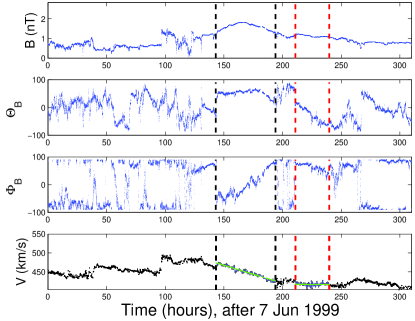
Figure 9: Example of two MCs in interaction. Magnetic cloud 44 is a large MC with a strong magnetic field; it is interacting with the smaller MC 26 (the vertical dashed lines define the MC boundaries). The magnetic field rotation is mostly in the longitude of the field ($\Phi_{B}$) for MC 44 and mostly in the latitude of the field ($\theta_{B}$) for MC 26 wich implies that the MC axis are almost orthogonal to each other. Nevertheless there is only a weak change in the magnetic field between the outward branch of MC 44 and the inward branch of MC 26. The MCs are separated by a sheath-like region with a magnetic field of different orientation. The bottom panel shows that MC 26 is not expanding. A linear least squares fit of the velocity is indicated by a green line in the time interval where an almost linear trend is present in each MC.

5.3 Interacting MCs

When, after the solar eruption of a magnetic cloud, another one is ejected having a more rapid velocity and in a similar direction to the first one, an interaction between the two MCs is expected near their encounter time. Depending of the relative orientations of the magnetic fields of the two interacting MCs, magnetic reconnection can develop during the interaction. Previous studies of these processes have been performed using observations of individual studied cases for both favorable conditions to the magnetic reconnection (e.g., Wang et al., 2005a), as well as non-reconnection conditions (e.g., Dasso et al., 2009). The dynamical evolution during the interaction of two magnetic clouds have been also studied numerically using MHD simulations (e.g., Lugaz et al., 2005; Xiong et al., 2007). These studies have typically found that a linear velocity profile is reached in the late evolution phase when the two MCs are traveling together.

We analyze these interacting MCs, with at least another MC in their vicinity, in the second subset of interacting MCs (I_MC). An example is shown in Fig. 9. The large MC 44 has a typical expanding rate ($\zeta=0.95$), while the smaller MC 26 located behind has no significant expansion ($\zeta\approx 0.$). A second couple of MCs have similar magnetic-field strengths ($<B>\approx 1$ nT), and the front MC 18 is in slight over-expansion ($\zeta=1.24$), while behind, MC 19 is in under-expansion ($\zeta=0.45$). A third couple of MCs is formed by MCs 15 and 42. The MC 15 was also detected by ACE spacecraft at 1 AU. Its expansion rate was classical ($\zeta=0.74$, Nakwacki et al., 2011). However, when the same MC is measured at 5.4 AU, it is strongly overtaken. In particular, its outward branch is compressed ($<B>\approx 1.2$ nT compared to $<B>\approx 0.5$ nT in its inward branch) and in under-expansion ($\zeta\approx 0.57$ compared to $\zeta=0.67$ in its inward branch). This MC 15 is overtaken by MC 42, which has a much stronger field ($<B>\approx 3$ nT) and is in strong over-expansion ($\zeta=2.35$).

Finally, the data set contains three MCs traveling close by. The three MCs (7,41,8) have similar magnetic field strengths, and this triad was identified as a single one ICME by Funsten et al. (1999) with an interval of counter-streaming electrons covering the full duration of the triad. All MCs are in over-expansion ($\zeta=3.2$, $1.94$, $1.5$, respectively), while the triad taken as a whole has an expansion rate closer to the mean value of all the MCs ($\zeta\approx 0.8$). Since this last $\zeta$ value is very different than the $\zeta$ values found within each MC, this triad of MCs is far from a relaxation state with a linear profile for the full time period (in contrast to the results of numerical simulations). At the same time, the three couples of MCs analyzed above also have significantly different $\zeta$ values as illustrated for one couple in Fig. 9.

The above three pairs and one triad of interacting MCs represent a variety of different cases. Their contrast with the simple evolution found in MHD simulations among similar flux ropes, is as follows. As with an overtaking fast flow, the MC in front is first compressed, so its expansion rate decreases (Lugaz et al., 2005; Xiong et al., 2007). The MCs 18 and 19, which have similar field strengths and sizes, are the closest to these simulations. However, the following MC is in under-expansion while it is the leading MC in (Lugaz et al., 2005; Xiong et al., 2007) MHD simulations.

When the magnetic reconnection is inhibited between the flux ropes (by nearly parallel magnetic fields), later on in the MHD simulations the couple of MCs travel together forming only one expanding structure, i.e. with a nearly linear velocity profile across both MCs (see Fig. 4 of Xiong et al., 2007). Such a case was not found in our data set.

Other MHD simulations have shown a more complex velocity pattern, for example in the case of the interaction of three flux ropes (see Fig. 6 of Lugaz et al., 2007). We still do not have a complete view of the interaction of MCs of various sizes, orientations, and magnetic helicities to help us interpret our observations of interacting MCs. We also have no information about the history of the interaction, which is crucial to improve our understanding of the local measurements since the above MHD simulations have shown that the interaction is a time-dependent process (even in the simplest interaction cases). Part of the history can be provided by other data sets such as those provided by heliospheric imagers and interplanetary radio data for a more recent time period (with the STEREO spacecraft).

6 Summary and conclusions

Our main goal in this paper has been to investigate how the MC properties, in particular their expansion rates, evolve in the outer heliosphere based on previous studies of the inner heliosphere and at 1 AU. During the travel from the Sun to the location of the in situ observations, the MC field may become partially reconnected with the overtaking magnetic field, as indicated by the presence of a back region in a large fraction of MCs. We have defined the MC boundaries to retain only the remaining flux rope part in order to analyze only the region that is not mixed with the SW.

Each observed MC has its own properties, with different temporal profiles of its magnetic field and its plasma parameters. Nevertheless we have found similarities between MCs that have allowed us to define three MC groups. The MCs within the first group have a radial velocity profile that ia almost linear with time, which implies that there is a self-similar expansion as theoretically expected, hence this group is referred to as non-perturbed (see examples in Fig. 1). In the second group, the temporal velocity profile can deviate significantly from linearity, hence they are perturbed (see examples in Fig. 2). Finally, we considered separately the MCs that have an extensive magnetic-field structure nearby, which are defined as the group in interaction (one example is shown in Fig. 9).

The perturbed MCs have an average size that is smaller than those of the non-perturbed MCs (Fig. 4a), while the opposite trend is true for the magnetic field strength, proton density, and temperature (Fig. 4b,c,5a). All of these results are consistent with perturbed MCs expanding less with solar distance than non-perturbed MCs, a property that has indeed been found independently from analyses of the in situ proton velocity (Fig. 6). For the proton $\beta$, we found no significant difference between these two MC groups (Fig. 5b).

The expansion in the radial direction (away from the Sun) is characterized by the non-dimensional parameter $\zeta$, defined by Eq. (5) from the in situ velocity profile. When the observed velocity profile is linear with time, the MC size has a power-law expansion such as $S\sim D^{\zeta}$ [Eq. (6) and following text]. For non-perturbed MCs, $\zeta$ has a narrow distribution ($\zeta=1.05\pm 0.34$). This is slightly larger than the values found in both the inner heliosphere ($0.91\pm 0.23$) and at 1 AU ($0.80\pm 0.18$). It is also larger than the global expansion exponent found from the analysis of the MC size versus helio-distance ($0.79\pm 0.46$). This lower exponent for the size could be due to the progressive pealing of the flux rope by reconnection or/and to a temporal evolution (Sect. 4.4).

The expansion rate of perturbed MCs, $\zeta=0.28\pm 0.52$, is on average significantly lower than for non-perturbed MCs, in quantitative agreement with previous results in the inner heliosphere. The rate $\zeta$ is also more variable within the group of perturbed MCs, such as in the inner heliosphere, with even one MC in over-expansion. These results agree with a temporal evolution of the expansion rate during the interaction with an overtaking flow as found in MHD simulations.

The MCs in interaction with a stronger magnetic field region have the largest variety of expansion rates $\zeta=1.00\pm 0.93$. Some of these MCs are in a rapid expansion stage (up to a factor of three bigger than for non-perturbed MCs), while one MC is even in compression. This wide variety of expansion rates is partially present in MHD simulations of interacting flux ropes or a flux rope overtaken by a fast stream: there is first a compression at the beginning of the interaction, followed by an increasingly high expansion rate with time that could become an over-expansion much latter on (with a magnitude that remains to be quantified). In all cases the properties of MCs that area in the process of interaction are difficult to interpret both because the past history is unknown and because they have a larger variety of properties than in MHD simulations.

Appendix A List of studied MCs

The studied MCs are listed in Table 3. We added the MCs 41 to 46, which were not present in the list of Rodriguez et al. (2004).

Table 3: List of MCs and their main properties.

MCa	$t_{c}$ b	Group c	$\theta$ d	$D$ d	$V_{c}$ e	$S$ e	$<B>$ f	$<N_{\rm p}>$ f	$<\beta_{p}>$ f	$\gamma$ g	$\zeta$ h
	d-m-y h:m (UT)		°	AU	km/s	AU	nT	cm-3		°
1	17-Jul-1992 19:46	interacting	-14	5.3	447	0.58	0.83	0.10	0.14	60	1.45
2	15-Nov-1992 23:18	perturbed	-20	5.2	595	1.39	0.91	0.04	0.12	82	0.50
3	11-Jun-1993 18:29	non-perturbed	-32	4.6	728	1.65	0.98	0.05	0.14	79	0.69
4	10-Feb-1994 16:46	interacting	-52	3.6	723	0.51	1.55	0.17	0.24	74	0.54
5	3-Feb-1995 21:05	perturbed	-22	1.4	754	0.25	4.33	1.26	0.21	55	0.50
6	15-Oct-1996 01:55	non-perturbed	24	4.6	673	1.30	0.64	0.04	0.11	67	0.89
7	10-Dec-1996 20:04	interacting	21	4.6	601	0.17	0.91	0.10	0.34	48	3.20
8	12-Dec-1996 22:45	interacting	20	4.7	512	0.29	0.94	0.14	0.31	65	1.50
9	09-Jan-1997 09:35	perturbed	19	4.7	471	0.36	2.05	0.42	0.10	40	0.41
10	27-May-1997 01:52	interacting	10	5.1	439	0.55	0.98	0.19	0.21	80	0.36
11	17-Aug-1997 09:59	perturbed	6	5.2	361	0.73	1.47	0.25	0.08	79	0.37
12	30-Aug-1997 19:26	perturbed	5	5.2	392	0.35	1.58	0.40	0.18	71	1.26
13	14-Nov-1997 19:18	non-perturbed	2	5.3	387	0.48	1.04	0.29	0.25	80	1.29
14	25-Jan-1998 20:24	perturbed	-2	5.4	379	0.05	1.72	0.24	0.08	53	-0.92
15	26-Mar-1998 22:53	interacting	-29	5.4	351	1.10	0.48	0.12	0.37	89	0.67
16	09-Apr-1998 20:34	perturbed	-6	5.4	411	0.24	0.58	0.36	0.71	68	0.54
17	15-Aug-1998 02:24	perturbed	-12	5.4	444	0.64	2.34	0.58	0.44	90	-0.18
18	27-Aug-1998 00:02	interacting	-13	5.4	389	0.37	0.91	0.16	0.15	73	1.24
19	30-Aug-1998 07:15	interacting	-13	5.4	377	0.49	1.10	0.22	0.16	71	0.45
20	8-Sep-1998 23:16	non-perturbed	-13	5.3	372	0.36	0.51	0.12	0.27	41	1.08
21	19-Sep-1998 02:19	interacting	-14	5.3	363	0.38	0.90	0.27	0.28	64	0.26
22	8-Oct-1998 16:35	non-perturbed	-15	5.3	401	0.82	0.95	0.04	0.03	85	0.88
23	9-Nov-1998 00:53	non-perturbed	-16	5.3	426	1.17	1.03	0.18	0.15	89	0.99
24	12-Nov-1998 16:16	interacting	-16	5.3	412	0.22	1.24	0.23	0.16	60	1.18
25	5-Mar-1999 01:18	perturbed	-22	5.1	454	0.63	2.72	0.27	0.14	86	1.05
26	16-Jun-1999 08:22	perturbed	-28	4.8	417	0.29	1.13	0.65	0.04	88	0.02
27	17-Aug-1999 06:46	interacting	-32	4.7	411	0.12	1.21	0.48	0.24	74	-0.81
28	31-Mar-2000 21:32	non-perturbed	-50	3.7	401	0.16	6.12	2.01	0.07	73	0.78
29	15-Jul-2000 14:52	non-perturbed	-62	3.2	500	0.41	0.29	0.06	0.73	21	1.14
30	11-Aug-2000 06:22	non-perturbed	-66	3.0	459	0.32	1.35	0.43	0.11	85	0.95
31	6-Dec-2000 23:15	non-perturbed	-80	2.2	394	0.23	2.84	0.80	0.08	31	1.70
32	12-Apr-2001 01:28	non-perturbed	-26	1.4	593	0.28	5.95	1.47	0.07	87	1.32
33	7-Jul-2001 13:35	interacting	40	1.4	296	0.20	4.18	8.51	0.67	81	0.33
34	24-Jul-2001 04:36	non-perturbed	51	1.5	381	0.42	5.17	2.39	0.16	30	0.58
35	24-Aug-2001 19:09	perturbed	68	1.7	539	0.13	8.78	2.70	0.06	88	0.48
36	14-Nov-2001 22:53	perturbed	75	2.3	632	0.32	2.77	0.18	0.03	79	0.67
37	12-Feb-2002 13:32	perturbed	58	2.9	519	0.20	4.73	1.76	0.11	58	0.06
38	5-May-2002 15:02	non-perturbed	46	3.4	385	0.16	1.87	0.82	0.09	70	1.57
39	16-Jun-2002 21:19	non-perturbed	41	3.6	658	1.49	2.85	0.17	0.02	70	0.73
40	18-Jul-2002 06:51	perturbed	38	3.8	530	0.08	3.54	0.51	0.04	79	0.00
41	11-Dec-1996 15:18	interacting	20	4.6	558	0.17	0.85	0.07	0.12	55	1.94
42	29-Mar-1998 07:06	interacting	-5	5.4	358	0.25	2.93	0.94	0.14	59	2.35
43	20-Apr-1998 12:38	perturbed	-6	5.4	416	0.30	1.64	0.28	0.13	65	-0.19
44	14-jun-1999 10:42	interacting	-28	4.8	450	0.55	1.60	0.21	0.09	58	0.95
45	17-Jan-2000 12:09	perturbed	-44	4.1	398	0.38	2.01	1.05	0.51	68	-0.08
46	27-Nov-2001 19:47	interacting	73	2.3	779	0.25	2.34	0.23	0.16	37	0.39

• Number identifying MCs.

• $t_{c}$ is the time of closest approach from the MC axis.

• The MCs are separated in three groups: non-perturbed, perturbed, and in interaction (denoted interacting).

• $\theta$ and $D$ are the latitude and solar distance.

• $V_{c}$ is the velocity at the closest distance from the MC axis and $S$ is the MC size. Both are computed in the radial direction away from the Sun ($\hat{\bf R}$).

• $<B>$, $<N_{\rm p}>$ and $<\beta_{p}>$ are the average over the flux rope of the field strength, the proton density and the proton $\beta$, respectively.

• $\gamma$ is the acute angle between the MC axis and the radial direction ($\hat{\bf R}$).

• $\zeta$ is the unidimensional expansion rate [Eq. (5)]. $\zeta<0$ means a MC observed in compression stage.