A spectral sequence on lattice homology

Abstract.

Using the link surgery formula for Heegaard Floer homology we find a spectral sequence from the lattice homology of a plumbing tree to the Heegaard Floer homology of the corresponding 3-manifold. This spectral sequence shows that for graphs with at most two “bad” vertices, the lattice homology is isomorphic to the Heegaard Floer homology of the underlying 3-manifold.

1. Introduction

Heegaard Floer homologies were introduced in 2001 by the first and third authors as invariants of closed, oriented 3-manifolds [17, 18]. The construction of the invariants relies on a choice of a Heegaard decomposition of the 3-manifold at hand, and then applies Lagrangian Floer homology to a symplectic manifold (and two Lagrangian subspaces of it) associated to the Heegaard decomposition. The theory comes in many variants: the version ${\rm{HF}}^{-}(Y)$ is the most powerful in 3- and 4-dimensional applications, while the simpler ${\widehat{\rm{HF}}}(Y)$ turnes out to be more accessible for computation. Since the introduction of the invariants, many results have been found towards their computability [3, 6, 13, 23], but a convenient computational scheme in general is still missing. For 3-manifolds which can be presented as the boundary of a negative definite plumbing with at most one bad vertex (in the sense of Definition 2.1), a relatively simple computational algorithm was described in [16].

Motivated by the result of [16], in [8] András Némethi introduced an algebraic object, the lattice homology for plumbed 3-manifolds, which — when considered for negative definite plumbings — provides a bridge between certain analytic properties of the singularity with resolution the given plumbing, and the differential topology of the boundary 3-manifold. Since lattice homology extends the combinatorial approach found in [16] to more general plumbings, it can be shown that for a negative definite plumbing tree $G$ with at most one bad vertex, the lattice homology ${\mathbb{HF}}^{-}(G)$ and the Heegaard Floer homology group ${\rm{HF}}^{-}(Y_{G})$ of the plumbed 3-manifold $Y_{G}$ (obtained by plumbing circle bundles over spheres according to $G$) are isomorphic. Indeed, Némethi extended the isomorphism of [16] to a larger class of plumbing graphs which he called almost-rational [8]. (For the definition of these notions, see Section 2. See also [11] for related results.) His results can be viewed as evidence for a conjecture that, for a plumbing tree $G$, the lattice homology ${\mathbb{HF}}^{-}(G)$ is isomorphic to the Heegaard Floer homology ${\rm{HF}}^{-}(Y_{G})$ of the corresponding 3-manifold $Y_{G}$. Further evidence to the validity of this conjecture is provided by the proof of a surgery exact triangle in lattice homology by Greene and (independently) by Némethi [2, 10], and by the introduction of knot lattice homology [14], cf. also [15].

In the present paper we show the existence of a spectral sequence from the lattice homology of a tree $G$ to the Heegaard Floer homology of the corresponding plumbed 3-manifold $Y_{G}$. This spectral sequence is derived from the surgery presentation of Heegaard Floer homology from [5], compare also [20, 21]. In the statement below, the groups ${{{\mathbb{HF}}^{-}}}(G)$ and ${\mathbf{HF}}^{-}(Y_{G})$ denote the regular lattice and Heegaard Floer homologies after completion (with respect to the $U$ variable). For a definition of ${\mathbb{HF}}^{-}(G)$ see Section 3. When the 3-manifold $Y_{G}$ is a rational homology sphere then the completed versions of the homologies determine the ones defined over the polynomial ring, cf. [5]; moveover, the closed four-manifold invariants can be defined using only the completed theory. The main result of the paper is:

Theorem 1.1.

Suppose that $G$ is a plumbing tree of spheres, and let $Y_{G}$ be the corresponding $3$-manifold. Then there is a spectral sequence $\{E_{i}\}_{i=1}^{\infty}$ with the properties:

• The $E_{2}$-term of the spectral sequence is isomorphic to the lattice homology ${{{\mathbb{HF}}^{-}}}(G)$.

• The spectral sequence converges to ${\rm{\mathbf{HF}}}^{-}(Y_{G})$.

• The lattice homology ${\mathbb{HF}}^{-}(G)$ naturally splits according to $\operatorname{Spin^{c}}$ structures over $Y_{G}$ (see text preceding Definition 3.6); similarly, ${\mathbf{HF}}^{-}(Y_{G})$ splits according to $\operatorname{Spin^{c}}$ structures. The spectral sequence respects these splittings.

• If $\mathbf{s}\in\operatorname{Spin^{c}}(Y_{G})$ is a torsion $\operatorname{Spin^{c}}$ structure (e.g. if $Y_{G}$ is a rational homology sphere, this holds for any $\mathbf{s}\in\operatorname{Spin^{c}}(Y_{G})$), the isomorphism of the $E_{2}$-term with ${\mathbb{HF}}^{-}(G)$ preserves the absolute Maslov grading.

• If $\mathbf{s}\in\operatorname{Spin^{c}}(Y_{G})$ is a non-torsion $\operatorname{Spin^{c}}$ structure, the isomorphism of the $E_{2}$-term with ${\mathbb{HF}}^{-}(G)$ preserves the relative Maslov grading.

Remark 1.2.

The $E_{\infty}$ term of the above spectral sequence (as a sequence of modules over $\mathbb{F}[[U]]$) recovers ${\rm{\mathbf{HF}}}^{-}(Y_{G})$ only as a vector space over $\mathbb{F}$. More information about the $\mathbb{F}[[U]]$-module structure can be obtained by applying an analogous spectral sequence over $\mathbb{F}[[U]]/U^{n}$, see Theorem 4.11 below, and also the proof of Corollary 1.3.

As an application, we derive the following result. (For the defintion of type-$n$ graphs, see Definition 2.1 in Section 2. Negative definite type-$n$ graphs include graphs with at most $n$ bad vertices.) See [11, Section 8] for special cases of this result.

Corollary 1.3.

If a plumbing tree $G$ is of type-2 then the lattice homology of $G$ is isomorphic to the Heegaard Floer homology of the underlying 3-manifold $Y_{G}$.

The paper is organized as follows. In Section 2 we fix notations and describe some necessary definitions, while in Section 3 we recall the basic concepts of lattice homology. Section 4 is devoted to the discussion of the spectral sequence, and finally in Section 5 we prove Corollary 1.3. In this proof we use the surgery exact sequence of Greene and Némethi [2, 10]. For completeness, in an Appendix we include a proof of this result adapted to the conventions used throughout our paper.

Acknowledgements: PSO was supported by NSF grant number DMS-0804121. AS was supported by OTKA NK81203, by the ERC Grant LDTBud and by the Lendület program. ZSz was supported by NSF grants number DMS-0603940, DMS-0704053, DMS-1006006.

2. Background

Suppose that $\Gamma$ is a tree on the vertex set $V=\mathrm{Vert}(\Gamma)=\{v_{1},\ldots,v_{n}\}$, while $G$ is the same graph together with an integer $m_{v}\in\mathbb{Z}$ (a framing) attached to each vertex $v$ of $\Gamma$. Let $M_{G}$ denote the associated incidence matrix (with framings in the diagonal). The plumbing 4-manifold defined by $G$ (when we plumb disk bundles over spheres according to $G$) will be denoted by $X_{G}$, and its boundary 3-manifold is $Y_{G}$. It is not hard to see that $M_{G}$ is the intersection matrix of the 4-manifold $X_{G}$ in the basis $\{E_{1},\ldots,E_{n}\}\subset H_{2}(X_{G};\mathbb{Z})$ where $E_{i}$ corresponds to the vertex $v_{i}$ ($i=1,\ldots,n$). Let $d_{v}$ denote the number of neighbours of a vertex $v$ in the tree $G$; this quantity is sometimes called the degree (or valency) of the vertex $v_{i}$. Although lattice homology can be defined for graphs containing cycles, in the present work we will restrict our attention to trees and forests (disjoint unions of trees).

Definition 2.1.

• Suppose that $G$ is a negative definite plumbing tree (that is, the matrix $M_{G}$ is negative definite). According to [1] there is a class $Z=\sum_{i}n_{i}E_{i}$ with $n_{i}\geq 0$ integers and $Z\neq 0$ which satisfies $Z\cdot E_{i}\leq 0$ for all $i$, and for any other class $Z^{\prime}=\sum_{i}n_{i}^{\prime}E_{i}$ with these properties $n_{i}\leq n_{i}^{\prime}$ holds for all $i$. The plumbing tree $G$ is called rational if for $Z=\sum_{i}n_{i}E_{i}$ we have

  $$(\sum_{i}n_{i}E_{i})^{2}=2\sum_{i}n_{i}+\sum_{i}n_{i}E_{i}^{2}-2.$$

  (This condition is equivalent to requiring that the geometric genus $p(Z)=\frac{1}{2}(Z^{2}+K\cdot Z)+1$ of the class $Z$ vanishes.)

• The vertex $v$ is a bad vertex of $G$ if $d_{v}+m_{v}>0$, i.e. the valency of the vertex is more than the negative of its framing.

• The plumbing tree $G$ is of type-$k$ if it has $k$ vertices $\{v_{i_{1}},\ldots,v_{i_{k}}\}$ on which we can change the framings $\{m_{i_{1}},\ldots,m_{i_{k}}\}$ in such a way that the result is rational.

Remark 2.2.

The above definition differs from the definition of Némethi [7]: we use the term bad vertices as it was used in [16]. For negative definite trees, the notion of almost-rational coincides with type-1. If a negative definite tree $G$ has $k$ bad vertices then it is of type-$k$. The converse is false, cf. the example of Figure 1.

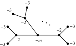
Figure 1. The plumbing diagram of the figure has at least $n$ bad vertices (where $n$ is the valency of the central $(-m)$-framed vertex) and it is either type-1 or rational (depending on the actual value of $m$). Notice that all the $(-2)$-framed vertices are bad vertices (in the sense of Definition 2.1). On the other hand, for $m$ sufficiently negative the graph is rational: let $K$ be the vector which is the sum of all $-3$-spheres, twice the $-2$ spheres, and once the central vertex. It follows that for any value of $m$ the graph is of type-1.

Recall that a plumbing tree also provides a surgery diagram for the 3-manifold it represents: replace each vertex of the diagram with an unknot, and arrange them so that two unknots link if and only if the corresponding vertices are connected by an edge. The framings of the unknots are given by the integers attached to the vertices of the plumbing graph. Notice that (viewing the resulting framed link $L=(L_{1},\ldots,L_{\ell})$ as a Kirby diagram) this procedure actually gives the 4-manifold $X_{G}$ with the given 3-dimensional boundary $Y_{G}$. In addition, if $L^{\prime},L^{\prime\prime}$ are two sublinks of the resulting link $L$ in such a way that $L^{\prime}\subset L^{\prime\prime}$, then this surgery theoretic approach also provides a cobordism associated to the pair: attach the 4-dimensional 2-handles to $Y_{L^{\prime}}$ along the components of $L^{\prime\prime}-L^{\prime}$ with the framings specified by $G$.

For later reference, let $\sigma(G)$ denote the signature of the intersection matrix $M_{G}$ (or equivalently, the 4-manifold $X_{G}$), and define $\chi(G)$ as the cardinality $|V|$ of its vertex set. Notice that since $G$ is a tree, $\chi(G)$ is equal to the Euler characteristic of $X_{G}$ minus 1.

3. Review of lattice homology

For the sake of completeness we review the basic notions of lattice homology. This notion was introduced by Némethi [8] (see also [9, 11]). The current presentation is similar to the one discussed in [14], with the difference that now we consider the completed version of the theory, cf. Remark 3.5. Let $G$ be a given plumbing tree/forest. Recall that $G$ is specified by a graph $\Gamma$, together with a map $m$ from the vertices $\mathrm{Vert}(G)$ to $\mathbb{Z}$, and the integer $m(v)=m_{v}$ is called the framing of $v$.

Next we recall the definition of the completed version of the lattice homology group of $G$. The group ${\mathbb{HF}}^{-}(G)$ is computed as the homology of the combinatorial chain complex ${\mathbb{CF}}^{-}(G)$, which is a module over the ring $\mathbb{F}[[U]]$ of formal power series (where $\mathbb{F}\cong{\mathbb{Z}}/{2}{\mathbb{Z}}$). To define it, let $\mathrm{Char}(G)\subset H^{2}(X_{G};\mathbb{Z})$ denote the set of characteristic cohomology classes on the 4-manifold $X_{G}$; i.e., it is the subset of those $K\in H^{2}(X_{G})$ which have the property that

$$K\cdot c\equiv c\cdot c$$

for all $c\in H_{2}(X_{G};\mathbb{Z})$. Let ${\mathbb{P}}(V)$ be the power set of $V=\mathrm{Vert}(G)$, so that $E\in{\mathbb{P}}(V)$ simply means that $E\subset V$. Now, the $\mathbb{F}[[U]]$-module underlying ${\mathbb{CF}}^{-}(G)$ is the direct product

(3.1) $${{{\mathbb{CF}}^{-}}}(G)=\Pi_{[K,E]\in\mathrm{Char}(G)\times{\mathbb{P}}(V)}\mathbb{F}[[U]]\langle[K,E]\rangle.$$

${\mathbb{CF}}^{-}(G)$ naturally admits an integral grading, called the $\delta$-grading. The $\delta$-grading of an element $U^{i}\otimes[K,E]$ is given by the cardinality $|E|$ of the elements in $E$. This grading naturally descends to a ${\mathbb{Z}}/{2}{\mathbb{Z}}$-grading by considering only the parity of $|E|$.

We define the boundary map $\partial\colon{\mathbb{CF}}^{-}(G)\to{\mathbb{CF}}^{-}(G)$ as follows. Given a subset $I\subset E$, we define the $G$-weight $f([K,I])\in\mathbb{Z}$ of the pair $[K,I]$ by the formula

(3.2) $$2f([K,I])=\left(\sum_{v\in I}K(v)\right)+\left(\sum_{v\in I}v\right)\cdot\left(\sum_{v\in I}v\right).$$

Moreover, for a pair $[K,E]$, we define the minimal $G$-weight $g([K,E])$ by the formula $g([K,E])=\min\{f([K,I])\mid{I\subset E}\}$. Next, for the vertex $v\in E\subset V$ consider the quantities

$$A_{v}([K,E])=g([K,E-v])$$

and

$$B_{v}([K,E])=\min\{f([K,I])\mid{v\in I\subset E}\}=\left(\frac{K(v)+v\cdot v}{2}\right)+g([K+2v^{*},E-v]),$$

where $v^{*}$ denotes the Poincaré dual of the vertex $v$ (when $v$ is regarded as an element of the second homology $H_{2}(X_{G},Y_{G};\mathbb{Z})$ of the plumbing 4-manifold). It follows trivially from the definition that $\min\{A_{v}([K,E]),B_{v}([K,E])\}=g([K,E])$. Let

$$a_{v}[K,E]=A_{v}([K,E])-g([K,E]) b_{v}[K,E]=B_{v}([K,E])-g([K,E]).$$ and

(Now we have that $\min\{a_{v}[K,E],b_{v}[K,E]\}=0$.) We define the boundary map on ${\mathbb{CF}}^{-}(G)$ by the formula

(3.3) $${\partial[K,E]}=\sum_{v\in E}U^{a_{v}[K,E]}\otimes[K,E-v]+\sum_{v\in E}U^{b_{v}[K,E]}\otimes[K+2v^{*},E-v]$$

on $[K,E]$ and extend it to ${\mathbb{CF}}^{-}(G)$ $U$-equivariantly and linearly. It is obvious that the boundary map drops the $\delta$-grading by one. A simple calculation (cf. [14]) shows that

Lemma 3.1.

The pair $({\mathbb{CF}}^{-}(G),\partial)$ is a chain complex, that is, $\partial^{2}=0$. ∎

Definition 3.2.

The homology $H_{*}({\mathbb{CF}}^{-}(G),\partial)$ of the chain complex $({\mathbb{CF}}^{-}(G),\partial)$ is the lattice homology ${\mathbb{HF}}^{-}(G)$ of the plumbing graph $G$.

Lattice homology is the homology of an infinite direct product. Nonetheless, it enjoys the following finiteness property:

Proposition 3.3.

The lattice homology group ${\mathbb{HF}}^{-}(G)$ is a finitely generated $\mathbb{F}[[U]]$ module.

Proof.

This can be easily seen by induction on the number of bad vertices in $G$, using the long exact sequence in lattice homology ([2, 10], see also Corollary 6.8), and using the result for graphs with no bad vertices as in [8]. ∎

Remark 3.4.

A number of further variants can be introduced along the same lines: using the coefficient ring $\mathbb{F}[U^{-1},U]]$ (the field of fractions for the ring of formal power series in $U$) we get ${\mathbb{CF}}^{\infty}(G)$ and the corresponding homology theory ${\mathbb{HF}}^{\infty}(G)$. Notice that ${\mathbb{CF}}^{-}(G)$ is a subcomplex of ${\mathbb{CF}}^{\infty}(G)$, hence we can consider the quotient complex ${\mathbb{CF}}^{+}(G)$, whose homology is ${\mathbb{HF}}^{+}(G)$. Setting $U=0$ in ${\mathbb{CF}}^{-}(G)$ we get the homology theory ${\widehat{\mathbb{HF}}}(G)$, over the base ring $\mathbb{F}$. More generally, by setting $U^{n}=0$ ($n\in\mathbb{N}$) we get the version ${\widehat{\mathbb{HF}}}^{[n]}(G)$.

Remark 3.5.

The conventional definition of lattice homology considers direct sum as opposed to direct product in the definition of ${\mathbb{CF}}^{-}(G)$ given in (3.1). Also, the usual coefficient ring is the polynomial ring $\mathbb{F}[U]$ rather than $\mathbb{F}[[U]]$. With the changes in the present definition, in fact, we consider a completed version of the theory. If $G$ is negative definite, then the usual definition (given for example, in [8, 14]) and the one given above determine each other. This principle is not true in general, cf. the second example in 3.11. We found the description adapted in this paper to be in accord with the corresponding Heegaard Floer homology theories.

The relation

$$K\sim K^{\prime}\qquad{\mbox{if and only if }}\qquad K-K^{\prime}\in 2H^{2}(X_{G},Y_{G};\mathbb{Z})$$

splits the generators into equivalence classes: $U^{i}\otimes[K,E]$ and $U^{j}\otimes[K^{\prime},E^{\prime}]$ are equivalent if $K\sim K^{\prime}$. This relation then splits the the chain complex ${\mathbb{CF}}^{-}(G)$ as well, and the definition of the boundary map in (3.3) shows that the boundary map respects this splitting. Since $G$ is a tree, the 4-manifold $X_{G}$ is simply connected, an hence an element of $K\in\mathrm{Char}(G)$ specifies a $\operatorname{Spin^{c}}$ structure $\mathbf{t}_{K}$ on $X_{G}$, therefore (by restricting $\mathbf{t}_{K}$ to the boundary $Y_{G}$) induces a $\operatorname{Spin^{c}}$ structure $\mathbf{s}_{K}$ on $Y_{G}$. It is not hard to see that $K\sim K^{\prime}$ holds if and only if $\mathbf{s}_{K}$ and $\mathbf{s}_{K^{\prime}}$ are isomorphic $\operatorname{Spin^{c}}$ structures on $Y_{G}$. Hence both the chain complexes and the homologies defined above split according to the $\operatorname{Spin^{c}}$ structures of $Y_{G}$. Recall that ${\mathbb{CF}}^{-}(G)$ admits a $\delta$-grading (given for the generator $[K,E]$ by $|E|$), splitting the homologies further:

Definition 3.6.

For $i\geq 0$ define ${\mathbb{HF}}^{-}_{i}(G,\mathbf{s})$ as the subgroup of ${\mathbb{HF}}^{-}(G)$ spanned by those pairs $[K,E]$ for which $\mathbf{s}_{K}=\mathbf{s}$ and $|E|=i$.

Lattice homology has a further grading, the Maslov grading. This structure is simplest to describe in the case where the underlying $\operatorname{Spin^{c}}$ structure is torsion (i.e. the first Chern class of that $\operatorname{Spin^{c}}$ structure is a torsion cohomology class). We give the grading in that case first.

Suppose that the $\operatorname{Spin^{c}}$ structure $\mathbf{s}_{K}$ associated to a generator $U^{i}\otimes[K,E]$ is torsion. In this case define the Maslov grading ${\rm{gr}}(U^{i}\otimes[K,E])$ of a generator $U^{i}\otimes[K,E]$ of ${\mathbb{CF}}^{-}(G)$ as

(3.4) $${\rm{gr}}(U^{i}\otimes[K,E])=-2i+2g(K,E)+|E|+\frac{1}{4}(K^{2}-3\sigma(G)-2\chi(G)).$$

(Recall that $K^{2}$ is defined as the square of $nK$ divided by $n^{2}$, where $nK\in H^{2}(X_{G},Y_{G};\mathbb{Z})$ and therefore it admits a cup square. As a result we expect ${\rm{gr}}(U^{i}\otimes[K,E])$ to be a rational number rather than an integer.)

Lemma 3.7.

(cf. [14]) The boundary map drops the Maslov grading ${\rm{gr}}$ by one.

Proof.

Proceed separately for the two types of components of the boundary map. After obvious simplifications, according to the definition of $a_{v}[K,E]$ we have that

$${\rm{gr}}(U^{i}\otimes[K,E])-{\rm{gr}}(U^{i}\cdot U^{a_{v}[K,e]}\otimes[K,E-v])=$$

$$=2g([K,E])+|E|+2a_{v}[K,E]-2g([K,E-v])-|E-v|=1.$$

Similarly,

$${\rm{gr}}(U^{i}\otimes[K,E])-{\rm{gr}}(U^{i}\cdot U^{b_{v}[K,e]}\otimes[K+2v^{*},E-v])=1$$

follows from the same simplifications and the definition of $B_{v}([K,E])$. ∎

We will find it convenient to use the following terminology:

Definition 3.8.

A Maslov graded chain complex is a $\mathbb{Q}$-graded chain complex over $\mathbb{F}[[U]]$ with the property that

• the differential drops grading by one and

• multiplication by $U$ drops grading by two.

Lemma 3.7 and Equation (3.4) together say that for a torsion $\operatorname{Spin^{c}}$ srtucture $\mathbf{s}$ the grading $\mathrm{gr}$ gives ${\mathbb{CF}}^{-}(G,\mathbf{s})$ a Maslov grading, in the sense of Definition 3.8.

Lemma 3.9.

Suppose that $\mathbf{s}_{K}=\mathbf{s}_{K^{\prime}}$ is a torsion $\operatorname{Spin^{c}}$ structure. Then the difference

$${\rm{gr}}(U^{i}\otimes[K,E])-{\rm{gr}}(U^{j}\otimes[K^{\prime},E^{\prime}])$$

is an integer, and it is congruent $\mod 2$ to the difference $|E|-|E^{\prime}|$.

Proof.

In the difference the terms coming from $\sigma(G)$ and $\chi(G)$ cancel, and the ones originating from the $U$-exponents or from the $g$-function are obviously even. We claim that the difference $\frac{1}{4}(K^{2}-(K^{\prime})^{2})$ is also even. Since $\mathbf{s}_{K}=\mathbf{s}_{K^{\prime}}$, we have that $K^{\prime}=K+2x$ for some vector $x\in H^{2}(X_{G},Y_{G};\mathbb{Z})$, therefore

$$\frac{1}{4}(K^{2}-(K^{\prime})^{2})=x\cdot(K+x),$$

which is even since $K$ is characteristic. (Note that since $x$ is in the relative cohomology, the above product always makes sense.) The only remaing terms are $|E|-|E^{\prime}|$, verifying the statement. ∎

We turn now to the non-torsion case. In this case the term $K^{2}$ is not defined, since $nK$ is not in $H^{2}(X_{G},Y_{G};\mathbb{Z})$ for any non-zero $n$. Nevertheless, if $\mathbf{s}_{K}=\mathbf{s}_{K^{\prime}}$, we can still consider the difference $K^{2}-(K^{\prime})^{2}$ by writing it as $(K-K^{\prime})\cdot(K+K^{\prime})$. The assumption $\mathbf{s}_{K}=\mathbf{s}_{K^{\prime}}$ then ensures that $K-K^{\prime}$ admits a lift from $H^{2}(X_{G};\mathbb{Z})$ to $H^{2}(X_{G},Y_{G};\mathbb{Z})$, hence the above product makes sense. This provides a possibility of defining a relative Maslov grading. Notice, however, that the lift of $K-K^{\prime}$ is not unique in general: by the long exact sequence of the pair $(X_{G},Y_{G})$ the ambiguity for choosing such a lift lies in the group $H^{1}(Y_{G};\mathbb{Z})\cong H_{2}(Y_{G};\mathbb{Z})$. Suppose that $x$ is a lift of $\frac{1}{2}(K-K^{\prime})$ and $y\in H_{2}(Y_{G};\mathbb{Z})$. Then the difference we get for $K^{2}-(K^{\prime})^{2}$ by using $x$ or $x+y$ can be easily computed to be equal to $K|_{Y_{G}}(y)$. (If the restriction $K|_{Y_{G}}$ is torsion, then this evaulation is obviously zero, and we are in the previous situation of having absolute Maslov gradings in torsion $\operatorname{Spin^{c}}$ structures.) Therefore if $d$ denotes the divisibility of $K|_{Y_{G}}$ (that is, this cohomology class equals $d$-times a primitive one), then the value $K^{2}-(K^{\prime})^{2}$ is well-defined up to $4d$, hence the relative Maslov grading is well-defined modulo $d$ only. (Notice that for a characteristic cohomology class $K$ the divisibility $d$ of the restriction $K|_{Y_{G}}$ is always even.) In summary, we have:

Lemma 3.10.

Fix two generators $U^{i}\otimes[K,E]$ and $U^{j}\otimes[K^{\prime},E^{\prime}]$ and suppose that ${\mathbf{s}}_{K}={\mathbf{s}}_{K^{\prime}}$ is a non-torsion $\operatorname{Spin^{c}}$ structure over $Y_{G}$. Then, the relative Maslov grading

$$\mathrm{gr}(U^{i}\otimes[K,E],U^{j}\otimes[K^{\prime},E^{\prime}])=-2(i-j)+2g(K,E)-2g(K,E^{\prime})+|E|-|E^{\prime}|+\frac{1}{4}(K^{2}-(K^{\prime})^{2}),$$

gives a well-defined element of ${\mathbb{Q}}/{d}$, where $d$ denotes the divisibility of $c_{1}({\mathbf{s}}_{K})$. ∎

The proof of Lemma 3.7 readily adapts to the non-torsion case: in this case, the lattice complex is a relatively $\mathbb{Q}/d$-graded Maslov-graded complex.

Examples 3.11.

• Consider the example of the graph $G$ with a single vertex $v$, no edges and the decoration of the single vertex to be equal to $+1$. Then a characteristic cohomology class $K$ can be identified with the odd number $K(v)$ it takes as a value on $v$. The generators of ${\mathbb{CF}}^{-}(G)$ are then $[2n+1,\{v\}]$ and $[2n+1]$. The boundary of $[2n+1]$ is 0, while

  $$\partial[2n+1,\{v\}]=\left\{\begin{array}[]{ll}[2n+1]+U^{n+1}\otimes[2n+3]&{\text{if $n\geq-1$}}\\ U^{-(n+1)}\otimes[2n+1]+[2n+3]&{\text{if $n<-1$}}.\end{array}\right.$$

  The map $\partial$ is then obviously injective on the subspace given by the finite sums of elements of the form $[2n+1,v]$. By allowing infinite sums (as we did), the element

  $$\sum_{n=-\infty}^{-1}U^{\frac{1}{2}(n+1)(n+2)}[2n+1,v]+\sum_{n=0}^{\infty}U^{\frac{1}{2}n(n+1)}[2n+1,v]$$

  generates ${{{\mathbb{HF}}^{-}}}(G)$ over $\mathbb{F}[[U]]$. This shows that in this case ${\mathbb{HF}}^{-}(G)={\mathbb{HF}}^{-}_{1}(G)=\mathbb{F}[[U]]$. A simple calculation shows that this element has zero Maslov grading, in accordance with the Heegaard Floer homological computation for the plumbing manifold $Y_{G}$ given by $G$, which is diffeomorphic to $S^{3}$.

• In the next example we assume that $G$ still has a single vertex $v$ (and no edges) and the framing of the single vertex is zero. The underlying 3-manifold is now $S^{1}\times S^{2}$. The generators are of the form $[2n]$ and $[2n,v]$, and two generators are in the same $\operatorname{Spin^{c}}$ structure if and only if the characteristic cohomology classes coincide. As always, $\partial[2n]=0$. A simple calculation shows that

  $$\partial[2n,v]=(1+U^{n})[2n].$$

  Considering the theory over $\mathbb{F}[U]$ (and allowing only finite sums) the homology for the $\operatorname{Spin^{c}}$ structure $n\neq 0$ is $\mathbb{F}[U]/(U^{n})$, while for $n=0$ it is $\mathbb{F}[U]\oplus\mathbb{F}[U]$. Working with the completed groups (and hence using the coefficient ring $\mathbb{F}[[U]]$), the term $(1+U^{n})$ is invertible for $n\neq 0$ (and vanishes if $n=0$), hence according to the definition we adopted in the present paper we have that ${\mathbb{HF}}^{-}(G,\mathbf{s}_{n})=0$ if $n\neq 0$ and ${\mathbb{HF}}^{-}(G,\mathbf{s}_{0})=\mathbb{F}[[U]]\oplus\mathbb{F}[[U]]$. (A simple computation shows that the Maslov gradings of the two generators are $\frac{1}{2}$ and $-\frac{1}{2}$.) Moreover, ${\mathbb{HF}}^{-}_{0}(G,\mathbf{s}_{0})\cong\mathbb{F}[[U]]$ and ${\mathbb{HF}}^{-}_{1}(G,\mathbf{s}_{0})\cong\mathbb{F}[[U]]$.

  This simple computation shows that for non-torsion $\operatorname{Spin^{c}}$ structures the completed theory (over the ring $\mathbb{F}[[U]]$) loses some information. On the other hand, for torsion $\operatorname{Spin^{c}}$ structures the completed theory determines the one referred to in Remark 3.5 (which is defined over $\mathbb{F}[U]$). We just note here that the resulting homologies are again isomorphic to the corresponding completed Heegaard Floer homology groups.

4. The spectral sequence

Before turning to the proof of our main result, we need to recall some definitions and constructions from [5] (cf. also [19]). Recall that the plumbing graph determines a link $L=(L_{1},\ldots,L_{\ell})$ in $S^{3}$: each vertex of the plumbing tree gives rise to an unknot and these unknots are linked if and only if the corresponding vertices are connected in the graph by an edge.

4.1. Constructions from link Floer homology

Let $H$ denote the homology group $H_{1}(S^{3}-L;\mathbb{Z})$. By fixing an orientation on the component $L_{i}$, it gives rise to an oriented meridian $\mu_{i}$, and these meridians generate $H$. Using these meridians we can identify the group ring $\mathbb{Z}[H]$ with the ring of Laurent polynomials on $\ell$ variables. Define $\mathbb{H}(L)$ as

$$\{\sum a_{i}\cdot[\mu_{i}]\mid a_{i}\in\mathbb{Q},\quad{\mbox{and}}\quad 2a_{i}+\ell k(L_{i},L-L_{i})\in 2\mathbb{Z}\},$$

where $\ell k(L_{i},L-L_{i})$ is the linking number of the component $L_{i}$ with the rest of the link. As it was discussed in [5, 19], the set $\mathbb{H}(L)$ parametrizes the relative $\operatorname{Spin^{c}}$ structures on $S^{3}-L$.

Fix a multi-pointed Heegaard diagram ${\mathcal{H}}=(\Sigma,\mbox{\boldmath$\alpha$},\mbox{\boldmath$\beta$},\mathbf{w},\mathbf{z})$ representing the link $L$, as in [19]. In this diagram $\mathbf{w}=(w_{1},\dots,w_{\ell})$ and $\mathbf{z}=(z_{1},\dots,z_{\ell})$ are basepoints with the property that the pair $w_{i}$ and $z_{i}$ represents the $i^{th}$ component of $L$. Recall that the multi-diagram in fact specifies an orientation on the link. When we wish to underscore this structure, we write an oriented link as $\vec{L}$.

Given the Heegaard diagram and a choice of $\mathbf{s}\in\mathbb{H}(L)$, we define the chain complex $\mathfrak{A}^{-}({\mathcal{H}},\mathbf{s})$ as follows. Any intersection point $\mathbf{x}\in{\mathbb{T}}_{\alpha}\cap{\mathbb{T}}_{\beta}$ has a Maslov grading $M(\mathbf{x})\in\mathbb{Z}$ (since the link $L$ is in $S^{3}$) and an Alexander multi-grading $A(\mathbf{x})\in\mathbb{H}(L)$, defined using the Heegaard diagram. This Alexander multi-grading is specified (up to an overall additive constant, i.e. by a vector), as follows. If $w_{i}$ and $z_{i}$ are the pair of basepoints belonging to the $i^{th}$ component of the link, and $\phi\in\pi_{2}(\mathbf{x},\mathbf{y})$ is any homotopy class connecting $\mathbf{x}$ and $\mathbf{y}$, then the $i^{th}$ component $A_{i}(\mathbf{x})$ of $A(\mathbf{x})$ satisfies

$$A_{i}(\mathbf{x})-A_{i}(\mathbf{y})=n_{z_{i}}(\phi)-n_{w_{i}}(\phi).$$

In an integral homology sphere (and specifically in $S^{3}$) such $\phi$ always exists and the difference above is independent of the choice of $\phi$.

Given $\mathbf{s}=(s_{1},\dots,s_{\ell})$ and $\phi$, we define the $\mathbf{s}$-modified multiplicity of $\phi\in\pi_{2}(\mathbf{x},\mathbf{y})$ by the formulas:

(4.1) $$E^{i}_{\mathbf{s}}(\phi) = \max\{s_{i}-A_{i}(\mathbf{x}),0\}-\max\{s_{i}-A_{i}(\mathbf{y}),0\}+n_{z_{i}}(\phi)$$

(4.2) $$= \max\{A_{i}(\mathbf{x})-s_{i},0\}-\max\{A_{i}(\mathbf{y})-s_{i},0\}+n_{w_{i}}(\phi).$$

This quantity has the following two properties:

• $E^{i}_{s}(\phi)\geq 0$ if all the local multiplicities of $\phi$ are non-negative.

• If $\phi_{1}\in\pi_{2}(\mathbf{p},\mathbf{q})$ and $\phi_{2}\in\pi_{2}(\mathbf{q},\mathbf{r})$, then for $\phi_{1}*\phi_{2}\in\pi_{2}(\mathbf{p},\mathbf{r})$

  $$E^{i}_{s}(\phi_{1}*\phi_{2})=E^{i}_{s}(\phi_{1})+E^{i}_{s}(\phi_{2}).$$

Given $\mathbf{s}=(s_{1},\dots,s_{\ell})\in\mathbb{H}(L)$, we define the corresponding chain complex $\mathfrak{A}^{-}({\mathcal{H}},\mathbf{s})$, which is a free module over the algebra $\mathbb{A}=\mathbb{F}[[U_{1},\dots,U_{\ell}]]$ generated by ${\mathbb{T}}_{\alpha}\cap{\mathbb{T}}_{\beta}$, and equipped with the differential:

(4.3) $$\partial\mathbf{x}=\sum_{\mathbf{y}\in{\mathbb{T}}_{\alpha}\cap{\mathbb{T}}_{\beta}}\sum_{\begin{subarray}{c}\phi\in\pi_{2}(\mathbf{x},\mathbf{y})\\ \mu(\phi)=1\end{subarray}}\#\left(\frac{{\mathcal{M}}(\phi)}{\mathbb{R}}\right)\cdot U_{1}^{E^{1}_{s_{1}}(\phi)}\cdots U_{\ell}^{E^{\ell}_{s_{\ell}}(\phi)}\cdot\mathbf{y}.$$

Note that this complex also depends on the choice of a suitable almost complex structure on the symmetric product. We suppress this almost complex structure from the notation for simplicity.

According to [5], the above complex is related to the Heegaard Floer homology of the 3-manifold obtained as sufficiently large surgeries on a link. (See also [20, 22] for the analogues for knots.) More formally, let $\Lambda=(\Lambda_{1},\ldots,\Lambda_{\ell})\in\mathbb{Z}^{\ell}$ be a vector of framings, and let $Y_{\Lambda}(L)$ denote the 3-manifold we get by performing $\Lambda_{i}$-surgery on $L_{i}$ for $i=1,\ldots,\ell$. Then, the following holds:

Theorem 4.1.

([5, Theorem 10.1]) If $\Lambda$ is sufficiently large (that is, for all $i$ the coordinate $\Lambda_{i}\in\mathbb{Z}$ is sufficiently large) then the Heegaard Floer chain complex ${\mathbf{CF}}^{-}(Y_{\Lambda}(L),\mathbf{s})$ is quasi-isomorphic to $\mathfrak{A}^{-}({\mathcal{H}},\mathbf{s})$. ∎

Although for general links $\mathfrak{A}^{-}({\mathcal{H}},\mathbf{s})$ can be challenging to compute, in the case where $L$ is the link diagram associated to a plumbing tree, the complex $\mathfrak{A}^{-}({\mathcal{H}},\mathbf{s})$ can be easily determined with the help of the above theorem. Recall that an $L$-space is a rational homology 3-sphere $Y$ with the property that for each $\operatorname{Spin^{c}}$ structure $\mathbf{s}$ over $Y$, the Heegaard Floer homology ${\rm{\mathbf{HF}}}^{-}(Y,\mathbf{s})\cong\mathbb{F}[[U]]$.

Lemma 4.2.

Let $G$ be a plumbing tree and $L$ be its corresponding link in $S^{3}$. Then, for each ${\mathbf{s}}\in{\mathbb{H}}(L)$, there is a homotopy equivalence $\mathfrak{A}^{-}({\mathcal{H}},{\mathbf{s}})\simeq\mathbb{F}[[U]]$.

Proof.

By Theorem 4.1 (which is identical to [5, Theorem 10.1]), $\mathfrak{A}^{-}({\mathcal{H}},{\mathbf{s}})$ computes the Heegaard Floer homology of a 3-manifold obtained by sufficiently positive surgeries on $L$. By [16, Lemma 2.6], this 3-manifold is an $L$-space, providing the desired isomorphism. ∎

The result given in [5, Theorem 7.7] (restated in Theorem 4.3 below) provides a chain complex, described in terms of the $\mathfrak{A}^{-}({\mathcal{H}},\mathbf{s})$ from above, which computes the Heegaard Floer homology of arbitrary surgeries on $L$. To describe this, we need a little more notation. Let us fix $\Lambda=(\Lambda_{1},\ldots,\Lambda_{\ell})$. Let $M\subseteq L$ be a sublink with $m$ components. The projection map

$$\psi^{M}\colon\mathbb{H}(L)\to\mathbb{H}(L-M)$$

is defined as follows. Label the components of $L=L_{1}\cup\dots\cup L_{\ell}$, and the components of $L-M=L_{j_{1}}\cup\dots\cup L_{j_{\ell-m}}$. We then define

$$\psi^{M}=(\psi^{M}_{j_{1}},\dots,\psi^{M}_{j_{\ell-m}})$$

by

$$\psi^{M}_{j_{i}}(\mathbf{s})=s_{j_{i}}-\frac{\ell k(L_{i},M)}{2}.$$

Here, $\ell k(L_{i},M)$ denotes the linking number of $L_{i}$ with $M$; recall that both are oriented (via an orientation induced from the ambient link $\vec{L}$).

As a module over $\mathbb{A}=\mathbb{F}[[U_{1},\ldots,U_{\ell}]]$, the surgery complex for the 3-manifold $Y_{\Lambda}(L)$ is defined by

(4.4) $$({\mathcal{C}}^{-}({\mathcal{H}},\Lambda),{\mathcal{D}}^{-})=\bigoplus_{M\subseteq L}\prod_{{\mathbf{s}}\in{\mathbb{H}}(L)}\mathfrak{A}^{-}({\mathcal{H}}^{L-M},\psi^{M}({\mathbf{s}})).$$

To define its differential, we need yet more notation. We need to give some algebraically defined maps, which are indexed by sublinks $M\subseteq L$, equipped with orientations (not necessarily agreeing with the induced orientation from $\vec{L}$). We write this data (sublink, together with a possibly different orientation) $\vec{M}$; and let $I_{+}(\vec{L},\vec{M})$ resp. $I_{-}(\vec{L},\vec{M})$ denote the sublink consisting of components of $M$ whose orientation (in $\vec{M}$) agree resp. disagree with the orentation on the ambient link $\vec{L}$. For a sublink $M\subseteq L$, we let $\Omega(M)$ denote the set of orientations on $M$.

Let $\overline{\mathbb{H}}(L)$ denote the extension of $\mathbb{H}(L)$, where we allow some of the components to be $\pm\infty$. For $i\in\{1,\dots,\ell\}$, we define a projection map $p^{\vec{M}}:\mathbb{H}(L)\to\overline{\mathbb{H}}(L)$ so that the $i^{th}$ component of $p^{\vec{M}}({\mathbf{s}})$ is specified by

$$\begin{cases}+\infty&\text{ if }i\in I_{+}(\vec{L},\vec{M}),\\ -\infty&\text{ if }i\in I_{-}(\vec{L},\vec{M}),\\ s_{i}&\text{ otherwise.}\end{cases}$$

There are algebraically defined maps

$${\mathcal{I}}^{\vec{M}}_{\mathbf{s}}:\mathfrak{A}^{-}({\mathcal{H}},{\mathbf{s}})\to\mathfrak{A}^{-}({\mathcal{H}},p^{\vec{M}}({\mathbf{s}}))$$

given by

$${\mathcal{I}}^{\vec{M}}_{\mathbf{s}}\mathbf{x}=\prod_{i\in I_{+}(\vec{L},\vec{M})}U_{i}^{\max(A_{i}(\mathbf{x})-s_{i},0)}\cdot\prod_{i\in I_{-}(\vec{L},\vec{M})}U_{i}^{\max(s_{i}-A_{i}(\mathbf{x}),0)}\cdot\mathbf{x}.$$

For each sublink $M\subset L$ fix a Heegaard diagram ${\mathcal{H}}^{L-M}$, and fix an orientation $\vec{M}$ on $M$. Let $J(M)\subset\overline{\mathbb{H}}(L)$ denote the subspace $\mathbf{s}=(s_{1},\dots,s_{\ell})$, for which $s_{i}=+\infty$ if $L_{i}\in I_{+}(M)$, and $s_{i}=-\infty$ if $L_{i}\in I_{-}(M)$. Counting holomorphic curves induces a homotopy equivalence

$$\theta^{\vec{M}}_{\mathbf{s}}\colon\mathfrak{A}^{-}({\mathcal{H}},p^{\vec{M}}({\mathbf{s}}))\to\mathfrak{A}^{-}({\mathcal{H}}^{L-M},\psi^{\vec{M}}({\mathbf{s}})).$$

(This homotopy equivalence was called ${\hat{D}}_{\mathbf{s}}^{\vec{M}}$ in [5]. We renamed it so that that it does not look like a differential.)

The differential on the surgery complex is given as a sum of components

$${\Phi}_{\mathbf{s}}^{\vec{M}}\colon\mathfrak{A}^{-}({\mathcal{H}},{\mathbf{s}})\to\mathfrak{A}^{-}({\mathcal{H}}^{L-M},\psi^{\vec{M}}({\mathbf{s}})),$$

defined by

$$\Phi_{\mathbf{s}}^{\vec{M}}=\theta^{\vec{M}}_{p^{\vec{M}}({\mathbf{s}})}\circ{\mathcal{I}}^{\vec{M}}_{\mathbf{s}}.$$

We now define the boundary operator ${\mathcal{D}}^{-}$ on the surgery complex as follows. For $\mathbf{s}\in\mathbb{H}(L)$ and $\mathbf{x}\in\mathfrak{A}^{-}({\mathcal{H}}^{L-M},\psi^{M}(\mathbf{s}))$, we set

$${\mathcal{D}}^{-}(\mathbf{s},\mathbf{x}) = \sum_{N\subseteq L-M}\sum_{\vec{N}\in\Omega(N)}(\mathbf{s}+\Lambda_{\vec{L},\vec{N}},\Phi^{\vec{N}}_{\psi^{M}(\mathbf{s})}(\mathbf{x}))$$

$$\in \bigoplus_{N\subseteq L-M}\bigoplus_{\vec{N}\in\Omega(N)}\mathfrak{A}^{-}({\mathcal{H}}^{L-M-N},\psi^{M\cup\vec{N}}(\mathbf{s}))\subseteq\mathfrak{A}^{-}({\mathcal{H}},\Lambda).$$

Of course, the homotopy equivalences $\theta^{\vec{M}}_{\mathbf{s}}$ appearing in the differential $\Phi_{\mathbf{s}}^{\vec{M}}$ are, in general, tricky to compute. For our present purposes, though, it turns out that a precise computation is unnecessary.

Recall that $({\mathcal{C}}^{-}({\mathcal{H}},\Lambda),{\mathcal{D}}^{-})$ is a module over $\mathbb{F}[[U_{1},\dots,U_{n}]]$. Choosing $U=U_{1}$, we can view it as a module over $\mathbb{F}[[U]]$ (it will turn out that our results are independent of the numbering of the $U_{i}$).

The complex $({\mathcal{C}}^{-}({\mathcal{H}},\Lambda),{\mathcal{D}}^{-})$ admits a natural splitting into summands, as follows. Consider the subspace $H(L,\Lambda)$ of $H_{1}(Y-L)$ spanned by framings $\Lambda_{i}$ of the components of $L$. The complex $({\mathcal{C}}^{-}({\mathcal{H}},\Lambda),{\mathcal{D}}^{-})$ naturally splits into summands indexed by the quotient space $\mathbb{H}(L)/H(L,\Lambda)$. In turn, this quotient space is naturally identified with $\operatorname{Spin^{c}}(Y,\Lambda)$, via for example, the filling construction from [19, Section 3.7].

One of the key results in [5] is the following:

Theorem 4.3.

([5, Theorem 7.7]) The homology of the chain complex $({\mathcal{C}}^{-}({\mathcal{H}},\Lambda),{\mathcal{D}}^{-})$ is identified with ${\mathbf{HF}}^{-}(Y_{G})$. Indeed, the identification respects the splitting of both spaces into summands indexed by $\operatorname{Spin^{c}}(Y_{G})$. ∎

The surgery complex has a natural filtration $S$ induced by the number of components in the sublink $M$. The differential ${\mathcal{D}}^{-}$ then splits as

$${\mathcal{D}}^{-}=\sum_{k=0}^{\infty}{\mathcal{D}}^{-}_{k},$$

where ${\mathcal{D}}^{-}_{k}$ is a term which drops the filtration level by exactly $k$. In particular, ${\mathcal{D}}^{-}_{0}$ is the differential on the associated graded complex.

By the $E_{1}$ term of the spectral sequence, we mean the chain complex whose underlying $\mathbb{F}[[U]]$-module is $H_{*}({\mathcal{C}}^{-}({\mathcal{H}},\Lambda),{\mathcal{D}}^{-}_{0})$, and whose differential is induced by ${\mathcal{D}}^{-}_{1}$.

Proposition 4.4.

The $E_{1}$ term in the filtration on $({\mathcal{C}}^{-}({\mathcal{H}},\Lambda),{\mathcal{D}}^{-})$ is identified with ${\mathbb{CF}}^{-}(G)$.

Proof.

Let us first identify the $\mathbb{F}[[U]]$-modules. Recall that $\mathrm{Vert}(G)$ can be used to index the components of $L$, therefore sublinks of $L$ naturally correspond subsets of $V=\mathrm{Vert}(G)$. Furthermore, a characteristic element $K$ specifies a $\operatorname{Spin^{c}}$ structure on $X_{G}$, and therefore an element $\mathbf{s}\in\mathbb{H}(L)$. By Lemma 4.2, we have that $H_{*}(\mathfrak{A}^{-}({\mathcal{H}}^{L-M},\psi^{M}({\mathbf{s}})))=\mathbb{F}[[U]]$. Mapping the generator $U^{i}\otimes[K,E]$ of ${\mathbb{CF}}^{-}(G)$ to $U^{i}$ in the factor $H_{*}(\mathfrak{A}^{-}({\mathcal{H}}^{L-M},\psi^{M}({\mathbf{s}})))$ of $H_{*}({\mathcal{C}}^{-}({\mathcal{H}},\Lambda),{\mathcal{D}}^{-}_{0})$ corresponding to the sublink $M$ indexed by $E$ and the $\operatorname{Spin^{c}}$ structure $\mathbf{s}$ corresponding to $K$, we get an isomorphism

$${\mathbb{CF}}^{-}(G)\to H_{*}({\mathcal{C}}^{-}({\mathcal{H}},\Lambda),{\mathcal{D}}^{-}_{0})$$

of $\mathbb{F}[[U]]$-modules.

Therefore, in order to verify the lemma, we need to identify ${\mathcal{D}}^{-}_{1}$ with the boundary operator $\partial$ of ${\mathbb{CF}}^{-}(G)$ described in Equation (3.3). Let $M^{\prime}\subseteq M$ denote a sublink with $|M|=|M^{\prime}|+1$. The boundary map ${\mathcal{D}}^{-}_{1}$ applied to an element of $H_{*}(\mathfrak{A}^{-}({\mathcal{H}}^{L-M},\psi^{M}({\mathbf{s}})))$ has two components in $H_{*}(\mathfrak{A}^{-}({\mathcal{H}}^{L-M^{\prime}},\psi^{M^{\prime}}({\mathbf{s}})))$, which correspond to the two orientations of the knot $M-M^{\prime}$. Let us denote the two components $d_{1}^{+}$ and $d_{1}^{-}$. Recall that $M-M^{\prime}$ is a knot, and hence it corresponds to some vertex $v$ of the plumbing graph $G$. Although $M^{\prime}-M$ is the unknot in $S^{3}$, in $Y_{M}$ it represents a possibly complicated knot, which we denote $K_{v}\subset Y_{M}$.

The components $d_{-}$ and $d_{+}$ of the differential have an interpretation as a four-manifold invariant. Specifically, the following square commutes:

$$\begin{CD}H_{*}(\mathfrak{A}^{-}({\mathcal{H}}^{L-M},\psi^{M}({\mathbf{s}})))@>{d_{1}^{\pm}}>{}>H_{*}(\mathfrak{A}^{-}({\mathcal{H}}^{L-M^{\prime}},\psi^{M^{\prime}}({\mathbf{s}})))\\ @V{}V{}V@V{}V{}V\\ {\mathbf{HF}}^{-}(Y_{M})@>{\mathbf{t}_{\pm}}>{}>{\mathbf{HF}}^{-}(Y_{M^{\prime}})\end{CD}$$

Here, $Y_{M}$ resp. $Y_{M^{\prime}}$ denotes any sufficiently large positive surgery on $M$ resp $M^{\prime}$, the vertical maps are the identifications from Lemma 4.2, the top horizontal map is either of the two maps $d_{1}^{\pm}$, and the bottom horizontal map is induced by the single two-handle cobordism $W$ from $Y_{M}$ to $Y_{M^{\prime}}$, equipped with one of the two $\operatorname{Spin^{c}}$ structures ${\mathbf{t}}_{+}$ or ${\mathbf{t}}_{-}$ of maximal square. An orientation on $M-M^{\prime}$ specifies which component $d^{\pm}_{1}$ we are using: when the orientation of $M-M^{\prime}$ agrees with that on $L$, we denote the component by $d^{+}_{1}$, and the other by $d^{-}_{1}$.

The orientation on $M-M^{\prime}$ also specifies which of the two maximal square $\operatorname{Spin^{c}}$ structures ${\mathbf{t}}_{\pm}$ we are using. Both ${\mathbf{t}}_{+}$ and ${\mathbf{t}}_{-}$ are $\operatorname{Spin^{c}}$ structures with maximal square, they have the same evaluation on $Y_{M}$, and

$${\mathbf{t}}_{+}={\mathbf{t}}_{-}+\mathrm{PD}[F],$$

where here $F\in H_{2}(W,Y_{M};\mathbb{Z})\cong\mathbb{Z}$ is the generator with the property that $\partial F\in H_{1}(Y_{M};\mathbb{Z})$ corresponds to our knot $M-M^{\prime}$ with its given orientation. (Commutativity of the above square is verified in [5, Theorem 10.2].)

Both of the top horizontal maps are clearly non-trivial (they are isomorphisms in all sufficiently large degrees), so they must both be multiplication by some power of $U$. We let $\alpha_{v}$ denote the $U$-power associated to $d^{+}_{1}$ and $\beta_{v}$ denote the $U$-power associated to $d^{-}_{1}$.

Lemma 4.5.

The exponents $\alpha_{v}$ and $\beta_{v}$ are independent of the surgery coefficients $\Lambda$.

Proof.

This is clear: the maps $d^{+}_{1}$ and $d^{-}_{1}$ make no reference to surgery coefficients. ∎

The same property holds on the lattice homology side:

Lemma 4.6.

Let $G$ and $G^{\prime}$ be two plumbing graphs, whose underlying graphs $\Gamma$ and $\Gamma^{\prime}$ coincide. Fix $K\in\mathrm{Char}(G)$, and $E\subset\mathrm{Vert}(G)=\mathrm{Vert}(G^{\prime})$, and $v\in E$. Let $K^{\prime}\in\mathrm{Char}(G^{\prime})$ be the characteristic vector with

$$K^{\prime}(v)+m^{\prime}_{v} =K(v)+m_{v}$$

$$K^{\prime}(w) =K(w)$$

for all $w\neq v$. Then,

$$a_{v}[K,E] =a_{v}[K^{\prime},E]$$

$$b_{v}[K,E] =b_{v}[K^{\prime}E]$$

Proof.

By Equation (3.2) and the choice of $K^{\prime}$, $f[K,I]=f[K^{\prime},I]$. Since $f$ determines $a_{v}$ and $b_{v}$, the claim follows. ∎

Lemma 4.7.

For sufficiently negative surgery coefficents along the sublink $M$ we have that $a_{v}=\alpha_{v}$ and $b_{v}=\beta_{v}$

Proof.

If the surgery coefficients along the sublink $M^{\prime}$ are sufficiently negative, the 3-manifold $Y_{M^{\prime}}$ is an $L$-space. Therefore the statement of the lemma is essentially [15, Proposition 4.1] (cf. [15, Remark 4.2]) applied to the graph $M^{\prime}$, where $v=M-M^{\prime}$ is the distinguished vertex. ∎

The identification stated in the proposition is equivalent to the statement that $a_{v}=\alpha_{v}$ and $b_{v}=\beta_{v}$ for the given framing $\Lambda$. This statement, however, is an immediate consequence of Lemmas 4.5, 4.6, and 4.7. ∎

Proposition 4.8.

The identification of Proposition 4.4 respects the (relative or absolute, depending on the $\operatorname{Spin^{c}}$ structure) Maslov gradings.

Proof.

Recall that in the proof of Proposition 4.4 the generator $[K,E]$ of ${\mathbb{CF}}^{-}(G)$ has been identified with the pair $\mathbf{s},M$, where $M$ is a sublink of the link $L$ defined by the plumbing graph $G$ and $\mathbf{s}$ is a relative $\operatorname{Spin^{c}}$ structure. In particular, $|M|=|E|$. We claim that this identification respects Maslov gradings. Indeed, if $K$ represents a torsion $\operatorname{Spin^{c}}$ structure, then the absolute Maslov grading of $[K,\emptyset]$ (thought of as an element of ${\mathbb{CF}}^{-}(G)$) coincides with that of $(\mathbf{s},\emptyset)$ (though of as an element of $({\mathcal{C}}^{-}({\mathcal{H}},\Lambda),{\mathcal{D}}^{-})$). Since the boundary map drops Maslov grading by one, the identification of Maslov gradings extends to all generators of the form $[K,E]$.

The same argument applies in the relatively graded setting (when $K$ restricts to a non-torsion class on $\partial X_{G}=Y_{G}$). ∎

We turn to Theorem 1.1:

Proof of Theorem 1.1.

Theorem 4.3 presents ${\mathbf{HF}}^{-}(Y_{G})$ as the homology of a filtered chain complex. Theorem 1.1 now follows from this theorem, together with the interpretation of the $E_{1}$ term on the filtration provided by Proposition 4.4. Proposition 4.8 then provides the proof of the claim about the identification of Maslov gradings. ∎

Certain higher differentials in the spectral sequence vanish for a priori reasons. This is most easily seen when one appeals to gradings.

Proposition 4.9.

The differential ${\mathcal{D}}^{-}_{2n}$ on the page $E_{2n}$ vanishes.

Proof.

Note first that all differentials on $E_{r}$ drop Maslov grading by $1$, and in particular change the Maslov grading by $1\pmod{2}$ (see Lemma 3.7). Looking at the expression of the grading $\mathrm{gr}$ on lattice homology, we see that the relative Maslov grading $\pmod{2}$ of any element $U^{i}\otimes[K,E]$ agrees with $|E|\pmod{2}$. Moreover, ${\mathcal{D}}^{-}_{k}$ drops $|E|$ by $k$. It follows from these observations and the identification of the Maslov gradings on the two theories (given by Proposition 4.8) that $D^{-}_{2n}$ vanishes. ∎

4.2. Module structures and the spectral sequence

After establishing Theorem 1.1, we need a slight further refinement in order to provide the proof of Corollary 1.3.

Suppose all the higher differentials on the spectral sequence appearing in Theorem 1.1 vanish. Even in this case we cannot necessarily conclude that ${\mathbf{HF}}^{-}(Y_{G})$ is computed by lattice homology: rather, ${\mathbf{HF}}^{-}(Y_{G})$ is determined up to extensions. This allows us to identify the two theories only as vector spaces over $\mathbb{F}$, but not as $\mathbb{F}[U]$-modules. In certain cases, this indeterminacy can be removed by working with coefficients in $\mathbb{F}[U]/U^{n}$ for all $n$. In the rest of the section we spell out the details of this observation.

The complex $({\mathcal{C}}^{[n]}({\mathcal{H}},\Lambda),{\mathcal{D}}_{[n]}^{-})$ will denote the complex over $\mathbb{F}[U]/U^{n}$ defined by taking the complex defined in Proposition 4.4, $({\mathcal{C}}({\mathcal{H}},\Lambda),{\mathcal{D}}^{-})$, and setting $U^{n}=0$. (Recall that we viewed $({\mathcal{C}}({\mathcal{H}},\Lambda),{\mathcal{D}}^{-})$ as a module over $\mathbb{F}[[U]]$ by defining the action by $U$ to be multiplication by $U_{1}$. To view it as a module over $\mathbb{F}[U]/U^{n}$, we must set $U_{1}^{n}=0$.) The complex $({\mathcal{C}}^{[n]}({\mathcal{H}},\Lambda),{\mathcal{D}}_{[n]}^{-})$ naturally inherits a filtration from $({\mathcal{C}}({\mathcal{H}},\Lambda),{\mathcal{D}}^{-})$.

Lemma 4.10.

Fix any positive integer $n$, and consider the spectral sequence on $({\mathcal{C}}^{[n]}({\mathcal{H}},\Lambda),{\mathcal{D}}_{[n]}^{-})$ induced from its filtration. This spectral sequence has $E_{1}$-term isomorphic to $\widehat{\mathbb{CF}}^{[n]}(G)$. ∎

Proof.

This is true because (thanks to Lemma 4.2) the $E_{1}$ term $H_{*}({\mathcal{C}}({\mathcal{H}},\Lambda),{\mathcal{D}}^{-}_{0})$ is torsion free, as an $\mathbb{F}[[U]]$-module. More explicitly, consider the filtered chain complex $C=({\mathcal{C}}({\mathcal{H}},\Lambda),{\mathcal{D}}^{-})$. The associated spectral sequence has $E_{1}=H_{*}(C,{\mathcal{D}}^{-}_{0})$, equipped with the differential induced by the ${\mathcal{D}}^{-}_{0}$-chain map ${\mathcal{D}}^{-}_{1}$.

The filtered chain complex $C^{\prime}=({\mathcal{C}}^{[n]}({\mathcal{H}},\Lambda),{\mathcal{D}}^{-}_{[n]})$ is gotten from $C$ by $C\otimes\mathbb{F}[U]/U^{n}$. In general, its $E_{1}$ term is computed by

$$E_{1}(C^{\prime})=H_{*}(C,{\mathcal{D}}^{-}_{0})\otimes\mathbb{F}[U]/U^{n})\oplus\mathrm{Tor}(H_{*}(C,{\mathcal{D}}^{-}_{0})\otimes\mathbb{F}[U]/U^{n}),$$

converging to $H_{*}(C^{\prime})$. In the case at hand, though, $H_{*}(C,{\mathcal{D}}^{-}_{0})$ is a direct product of Heegaard Floer homology groups of 3-manifolds obtained as large surgeries on various components of our link, each of which, according to Lemma 4.2, contributing a factor of $\mathbb{F}[[U]]$. Since $\mathrm{Tor}(\mathbb{F}[[U]],\mathbb{F}[U]/U^{n})=0$, we have that $\mathrm{Tor}(H_{*}(C,{\mathcal{D}}^{-}_{0})\otimes\mathbb{F}[U]/U^{n})=0$. It follows that $E_{1}(C^{\prime})=E_{1}(C)\otimes\mathbb{F}[U]/U^{n}$, equipped with the differential induced from ${\mathcal{D}}^{-}_{1}$. But this $E_{1}$ term is precisely $\widehat{\mathbb{CF}}^{[n]}(G)$. ∎

Now the version of Theorem 1.1 for the $U^{n}=0$ truncated theory has the following shape.

Theorem 4.11.

Suppose that $G$ is a plumbing tree of spheres, and let $Y_{G}$ be the corresponding $3$-manifold. Then there is a spectral sequence $\{E_{i}\}_{i=1}^{\infty}$ with the property that

• the $E_{2}$-term of the spectral sequence is isomorphic to the $U^{n}=0$-specialized lattice homology ${{{\widehat{\mathbb{HF}}}}^{[n]}}(G)$ and

• the spectral sequence converges to the $U^{n}=0$-specialized Heegaard Floer homology group ${\widehat{\rm{\mathbf{HF}}}}^{[n]}(Y_{G})$. ∎

Theorem 4.11 can be used to gain a little more information about the $\mathbb{F}[[U]]$-module structure on ${\mathbf{HF}}^{-}(Y_{G})$ (in terms of lattice homology). This improvement rests on the following algebraic result.

Lemma 4.12.

Suppose that $C$ and $C^{\prime}$ are two Maslov-graded chain complexes over $\mathbb{F}[[U]]$ whose homologies are finitely generated (as $\mathbb{F}[[U]]$-modules). If for all $n\geq 1$,

$$H_{*}(C\otimes\mathbb{F}[U]/U^{n})\cong H_{*}(C^{\prime}\otimes\mathbb{F}[U]/U^{n})$$

as $\mathbb{F}$-vector spaces, then it follows that $H_{*}(C)\cong H_{*}(C^{\prime})$ as $\mathbb{F}[[U]]$-modules.

Proof.

Fix a rational number $d$ and an integer $k>0$. Let $M(d,k)$ denote the Maslov-graded $\mathbb{F}[[U]]$-module with the following two properties:

• $M(d,k)\cong\mathbb{F}[U]/U^{k}$ as an $\mathbb{F}[[U]]$-module, and

• the generator of $M(d,k)$ has Maslov grading $d$ (i.e. the whole module is supported in Maslov gradings between $d$ and $d-2k$).

We extend the definition of $M(d,k)$ to $k=0$ to be the Maslov-graded $\mathbb{F}[[U]]$-module with the following two properties:

• $M(d,0)\cong\mathbb{F}[[U]]$ as an $\mathbb{F}[[U]]$-module, and

• the generator of $M(d,0)$ has Maslov grading $d$ (i.e. the whole module is supported in Maslov gradings $\leq d$).

Since $\mathbb{F}[[U]]$ is a principal ideal domain, the finitely-generated, Maslov-graded $\mathbb{F}[[U]]$-module $H_{*}(C)$ splits as the direct sum of modules of the form $M(d,k)$; i.e.

$$H_{*}(C)\cong\bigoplus_{d\in\mathbb{Q},k\in\{0,\dots,\infty\}}M(d,k)^{c_{d,k}},$$

where $c_{d,k}$ is a collection of non-negative integers, only finitely many of which are positive.

Our goal is to show that the collection of $\mathbb{F}$-vector spaces $\{H_{*}(C\otimes\mathbb{F}[U]/{U^{n}})\}_{n=0}^{\infty}$ uniquely determines the isomorphism type of $H_{*}(C)$ as an $\mathbb{F}[[U]]$-module, i.e. it uniquely determines the coefficients $\{c_{d,k}\}_{d,k}$.

This statement follows from an application of the universal coefficients theorem, stating that

(4.5) $$H_{*}(C\otimes\mathbb{F}[U]/U^{n})\cong(H_{*}(C)\otimes\mathbb{F}[U]/U^{n})\oplus\mathrm{Tor}_{*-2k-1}(H_{*}(C),\mathbb{F}[U]/U^{n}),$$

where the perhaps unfamiliar shift in grading (of $2k+1$, rather than simply $1$) on the $\mathrm{Tor}$ results from the fact that the action by $U$ shifts Maslov grading by $2$.

We find it convenient to encode the input data in terms of a two-variable generating function

$$P_{C}(s,t)=\sum_{n\geq 0,m}\dim_{\mathbb{F}}H_{m}(C\otimes\mathbb{F}[U]/U^{n})s^{n}t^{-m}.$$

By Equation (4.5),

$$P_{H_{*}(C)}=\sum_{d,k}c_{d,k}\cdot P_{M(d,k)},$$

where

$$P_{M(d,k)}=\sum_{n\geq 0,m}\dim_{\mathbb{F}}(M_{m}(d,k)\otimes\mathbb{F}[U]/U^{n})s^{n}t^{-m}+$$

$$t^{2k+1}\sum_{n\geq 0,m}\dim_{\mathbb{F}}(M_{m}(d,k)\otimes\mathbb{F}[U]/U^{n})s^{n}t^{-m}.$$

The lemma is proved once we show that the functions $P_{M(d,k)}$ are linearly independent (over $\mathbb{Z}$). This in turn follows form a straightforward calculation:

$$P_{M(d,k)}=t^{-d}\left(\frac{\sum_{i=0}^{k-1}(st^{2})^{i}}{1-s}+t^{2k+1}\frac{\sum_{i=0}^{k-1}s^{i}}{1-st^{2}}\right)=t^{-d}\left(\frac{1-(st^{2})^{k}+t^{2k+1}(1-s^{k})}{(1-s)(1-st^{2})}\right),$$

thought of as a rational function in $s$; and also

$$P_{M(d,0)}=\frac{t^{-d}}{(1-s)(1-st^{2})}.$$

Note that $(1-s)(1-st^{2})P_{M(d,k)}$ is a degree-$k$ polynomial in $s$. When $k>0$, the coefficient of $s^{k}$ is $-t^{-d}(t^{2k}+t^{2k+1})$, while at $k=0$, we get the constant (in $s$) polynomial $t^{-d}$. The linear independence of the $P_{M(d,k)}$ follows immediately. ∎

Remark 4.13.

A version of Lemma 4.12 applies when $C$ and $C^{\prime}$ are two relatively ${\mathbb{Z}}/{d}{\mathbb{Z}}$ Maslov-graded chain complexes, as well. In that case, the generating function $P_{M}(s,t)$ is defined over $\mathbb{Z}[{\mathbb{Z}}/{d}{\mathbb{Z}}][[s]]$; i.e. $t$ is a primitive $n^{th}$ root of unity.

Corollary 4.14.

Suppose that all higher differentials $D_{i}^{-}$ vanish for $i\geq 2$ in the spectral sequence associated to $({\mathcal{C}}^{-}({\mathcal{H}},\Lambda),{\mathcal{D}}^{-})$. Suppose that the same holds for all the truncated spectral sequences $({\mathcal{C}}^{[n]}({\mathcal{H}},\Lambda),{\mathcal{D}}^{-}_{[n]})$. Then, ${\mathbb{HF}}^{-}(G)$ and ${\mathbf{HF}}^{-}(Y_{G})$ are isomorphic as $\mathbb{F}[[U]]$-modules.

Proof.

This follows quickly from Lemma 4.12. ∎

5. Graphs of type-2

The proof of Corollary 1.3 relies on the following simple corollary of the existence of the surgery triangle for lattice homology. (The exact sequence we will use in the proof has been described by Greene [2, Theorem 3.1], and independently by Némethi [10]; see also the Appendix for a version adapted to the present notational conventions.)

Theorem 5.1.

Suppose that the plumbing tree $G$ is of type-$k$. Then ${\mathbb{HF}}^{-}_{q}(G)=0$ for $q>k$.

Proof.

The proof of the theorem proceeds by induction on $k$. For $k=0$ (i.e. if $G$ is rational), the claim follows from [8, Proposition 4.1.4.]. Suppose now that $G$ is of type-$(k+1)$ and assume that the claim of the theorem holds for graphs of type at most $k$. Let $v$ be a vertex of $G$ from the set $\{v_{i_{1}},\ldots,v_{i_{k+1}}\}$ appearing in Definition 2.1 of the type of $G$. Then, by the same definition, $G-v$ is of type-$k$. Let $G_{-n}$ denote the graph we get from $G$ by decreasing the framing of the chosen $v$ by $n\in{\mathbb{N}}$. If $n$ is sufficiently large, then (again by Definition 2.1) the graph $G_{-n}$ is of type-$k$. Fix now $q>k+1$ and consider the following portion of the long exact sequence associated to $(G_{-n},v)$ (cf. Corollary 6.8):

$$\ldots\to{\mathbb{HF}}^{-}_{q}(G_{-n})\to{\mathbb{HF}}^{-}_{q}(G_{-n+1})\to{\mathbb{HF}}^{-}_{q-1}(G-v)\to\ldots$$

By the inductive assumption, the first and the third terms vanish, hence by exactness so does the middle term. Iterating this argument until we get the given framing on $v$, the result follows and shows that ${\mathbb{HF}}^{-}_{q}(G)=0$ for $q>k+1$. ∎

In a similar manner, we get

Theorem 5.2.

If the plumbing tree $G$ is of type-$k$ then ${\widehat{\mathbb{HF}}}^{[n]}_{q}(G)=0$ for all $q>k$ and all $n\in\mathbb{N}$. ∎

Remark 5.3.

For $G$ negative definite, Theorem 5.1 can be sharpened to $q\geq k$. This strengthening, however, does not hold for the truncated theories ${\widehat{\mathbb{HF}}}^{[n]}(G)$, hence the negative definite assumption does not improve Theorem 5.2 in this sense.

From these results the proof of the corollary is a simple exercise:

Proof of Corollary 1.3.

Suppose that $G$ is a plumbing tree (or forest) of type-2 and consider the spectral sequence provided by Theorem 1.1. By Proposition 4.9 we have that $E_{2}=E_{3}$, and since by Theorem 5.1 the homology (and so the $E_{2}$-table of the spectral sequence) concentrates on the rows with $|E|$-gradings $0,1,2$, the higher differentials point from or to vanishing groups, implying that ${\mathcal{D}}^{-}_{i}=0$ for all $i\geq 3$. This means that $E_{2}=E_{\infty}$, hence by Theorem 1.1 the lattice and Heegaard Floer homologies coincide, as vector spaces over $\mathbb{F}$. To get the corresponding isomorphism as $\mathbb{F}[[U]]$-modules, we use the version of the spectral sequence over $\mathbb{F}[U]/U^{n}$, Theorem 4.11 cf. Corollary 4.14. For torsion $\operatorname{Spin^{c}}$ structures, the isomorphism of Maslov-graded $\mathbb{F}[[U]]$-modules follows now from Lemma 4.12. For non-torsion $\operatorname{Spin^{c}}$ structures, we appeal to the modification of the proof of Lemma 4.12 described in Remark 4.13. ∎

6. Appendix: the exact sequence

For completeness, in this final section we prove the exact sequences in lattice homology used above. These results could be derived from [2, 10], but we find it convenient to include this proof here, as it follows the conventions and formalism introduced in Section 3.

Let $G$ be a plumbing graph, and $v\in\mathrm{Vert}(G)$ be a distinguished vertex with framing $m_{v}$. $G-v$ will denote the graph obtained by omitting the vertex $v$. We define the extension map $\Phi_{v}\colon{\mathbb{CF}}^{-}(G-v)\to{\mathbb{CF}}^{-}(G)$ by the formula

(6.1) $$\Phi_{v}([K,E])=\sum_{p\equiv m_{v}\pmod{2}}[(K,p),E].$$

On the right-hand-side we write characteristic vectors for $G$ as pairs $(K,p)$, where $K$ is a characteristic vector for $G-v$, and $p$ is the evaluation of the characteristic vector on the distinguished vertex $v$. Since any component of $\Phi_{v}([K,E])$ determines $[K,E]$, it is easy to see that the above formula indeed provides a function on ${\mathbb{CF}}^{-}$ (meaning that any component of $\Phi_{v}(x)$ for a possibly infinite sum $x$ has coefficient in $\mathbb{F}[[U]]$). In fact, the above principle also shows that $\Phi_{v}$ is injective.

Lemma 6.1.

For each vertex $v\in\mathrm{Vert}(G)$, the map $\Phi_{v}$ is a chain map.

Proof.

This follows immediately from the fact that for any $E\subset G-v$, the $(G-v)$-weight $f_{G-v}[K,E]$ of the pair $[K,E]$ agrees with the $G$-weight $f_{G}[(K,p),E]$ of the pair $[(K,p),E]$ where $p$ is any integer with the allowed parity. (Here $f_{G-v}$ and $f_{G}$ refer to the function defined in Equation (3.2) with the respective graphs $G-v$ and $G$.) This implies that the corresponding functions $g_{G-v}$ and $g_{G}$ of minimal weights also coincide, and since the boundary maps are determined by these minimal weight functions, the result follows at once. ∎

Let $G_{+1}(v)$ denote the graph $G$ with the same framings, except on the vertex $v$ we consider $m_{v}+1$ instead of $m_{v}$. Define the map $\Psi_{v}\colon{\mathbb{CF}}^{-}(G)\to{\mathbb{CF}}^{-}(G_{+1}(v))$ by the formula

(6.2) $$\Psi_{v}[(K,p),E]=\sum_{m=-\infty}^{\infty}U^{s_{m}}\otimes[(K,p+2m-1),E],$$

where $s_{m}=g_{G_{+1}(v)}[(K,p+2m-1),E]-g_{G}[(K,p),E]+\frac{m(m-1)}{2}$. It is easy to see that when $v\not\in I\subset E$ the equality $f_{G_{+1}(v)}[(K,p+2m-1),I]=f_{G}[(K,p),I]$ holds, hence $s_{m}=\frac{m(m-1)}{2}\geq 0$ in this case. If $v\in I\subset E$ then $f_{G_{+1}(v)}[(K,p+2m-1),I]-f_{G}[(K,p),I]$ is at most $|m|$ in absolute value, hence after addig $\frac{m(m-1)}{2}$ to it, the result will be nonnegative. In conclusion, $s_{m}$ is nonnegative for any $(K,p)$ and $m$.

Once again, a short argument is needed to confirm that the above formula defines a function on ${\mathbb{CF}}^{-}$, that is, for an infinite sum $\sum_{i\in\mathbb{Z}}U^{m_{i}}[K_{i},E_{i}]$ all coordinates of the image admit a coefficient in $\mathbb{F}[[U]]$. This property follows from the fact that if $p+2m$ is fixed then the value $s_{m}$ converges to infinity as $m\to\pm\infty$, implying that at most finitely many terms $[(K,p+2m-1),E]$ with $p+2m$ fixed can have a given $U$-power in the image.

Lemma 6.2.

The map $\Psi_{v}$ is a chain map.

Before starting the proof of this lemma, we need to define one further map. Suppose that the graph $G_{e}$ is constructed from $G$ by adding a new vertex $e$ with framing $(-1)$ and an edge connecting $e$ and $v$. Consider the map

$$P\colon{\mathbb{CF}}^{-}(G_{e})\longrightarrow{\mathbb{CF}}^{-}(G_{+1}(v))$$

given by the formula:

$$P[(K,p,2m-1),E]=\left\{\begin{array}[]{ll}U^{s}\otimes[(K,p+2m-1),E]&{\text{if $e\not\in E$}}\\ 0&{\text{if $e\in E$,}}\end{array}\right.$$

where $s_{m}=g_{G_{+1}(v)}[(K,p+2m-1),E]-g_{G_{e}}[(K,p,2m-1),E]+\frac{m(m-1)}{2}$. (Once again, $(K,p,2m-1)$ denotes the cohomology class on $G_{e}$ which is $K$ on $G-v$, takes the value $p$ on $v$ and the value $2m-1$ on $e$.) As above, it can be verified that $P$ extends to a well-defined function on ${\mathbb{CF}}^{-}(G_{e})$.

Lemma 6.3.

The map $P$ is a chain map.

Proof.

We wish to prove that $\partial\circ P[(K,p,2m-1),E]=P\circ\partial[(K,p,2m-1),E].$ First, we consider the case where $e\in E$. In this case the left hand side is zero. Moreover,

$$P\circ\partial[(K,p,2m-1),E] = P(U^{a_{e}[(K,p,2m-1),E]}\otimes[(K,p,2m-1),E-e])$$

$$+P(U^{b_{e}[(K,p,2m-1),E]}\otimes[(K,p+2,2m-3),E-e])$$

$$= U^{d_{1}}\otimes[(K,p+2m-1),E-e]+U^{d_{2}}\otimes[(K,p+2m-1),E-e],$$

where

$$d_{1}=a_{e}[(K,p,2m-1),E]+g[(K,p+2m-1),E-e]-g[(K,p,2m-1),E-e]+\frac{m(m-1)}{2}$$

and

$$d_{2}=b_{e}[(K,p,2m-1),E]+g[(K,p+2m-1),E-e]-g[(K,p+2,2m-3),E-e]+2m^{2}-6m+4.$$

In fact, it is easy to see that

$$d_{1}=g[(K,p+2m-1),E-e]-g[(K,p,2m-1),E]+\frac{m(m-1)}{2}=d_{2},$$

so the two terms cancel.

Next, suppose that $e\not\in E$. Observe that

$$P\circ\partial[(K,p,2m-1),E]=$$

$$\sum_{w\in E}U^{c_{1}(w)}\otimes[(K,p+2m-1),E-w]+U^{d_{1}(w)}\otimes[(K,p+2m-1)+2w^{*},E-w],$$

and

$$\partial\circ P[(K,p,2m-1),E]=$$

$$\sum_{w\in E}U^{c_{2}(w)}\otimes[(K,p+2m-1),E-w]+U^{d_{2}(w)}\otimes[(K,p+2m-1)+2w^{*},E-w],$$

In fact, it is easy to see that

$$c_{1}(w)=g[(K,p+2m-1),E-w]-g[(K,p,2m-1),E]+\frac{m(m-1)}{2}=c_{2}(w)$$

and

$$d_{1}(w)=g[(K,p+2m-1),E-w]-g[(K,p,2m-1),E]+\frac{m(m-1)}{2}+\frac{L(w)+w\cdot w}{2}=d_{2}(w),$$

where $L=(K,p+2m-1)$ and $w\cdot w$ is taken in $G_{+1}(v)$. This completes the verification of the statement of the lemma. ∎

Proof of Lemma 6.2.

Consider now the map $\Phi_{e}\colon{\mathbb{CF}}^{-}(G)\to{\mathbb{CF}}^{-}(G_{e})$. The map $\Psi_{v}$ is simply the composition $P\circ\Phi_{e}$, and since both maps are chain maps, so is $\Psi_{v}$, concluding the proof of the lemma. ∎

Theorem 6.4.

For any $v\in G$, the $U$-equivariant maps $\Psi_{v}$ and $\Phi_{v}$ fit into a short exact sequence of chain complexes:

(6.3) $$0\longrightarrow{\mathbb{CF}}^{-}(G-v)\stackrel{{\scriptstyle\Phi_{v}}}{{\longrightarrow}}{\mathbb{CF}}^{-}(G)\stackrel{{\scriptstyle\Psi_{v}}}{{\longrightarrow}}{\mathbb{CF}}^{-}(G_{+1}(v)){\longrightarrow}0.$$

The theorem could be proved by a direct check of exactness at each term — we rather choose an alternative way of first dealing with the $U=0$ theory (and the corresponding result there) and then apply abstract reasoning to verify the theorem. Define the map $\widehat{\Phi}_{v}\colon\widehat{\mathbb{CF}}(G-v)\to\widehat{\mathbb{CF}}(G)$ corresponding to $\Phi_{v}$ by the same formula as given by (6.1). Next define $\widehat{\Psi}_{v}\colon\widehat{\mathbb{CF}}(G)\to\widehat{\mathbb{CF}}(G_{+1}(v))$ (corresponding to the map $\Psi_{v}$) by the same formula as given in Equation (6.2), after setting $U=0$.

Lemma 6.5.

The map $\widehat{\Psi}_{v}\colon\widehat{\mathbb{CF}}(G)\to\widehat{\mathbb{CF}}(G_{+1}(v))$ corresponding to $\Psi_{v}$ in the $U=0$ theory is given by the formula

$$\Psi_{v}([(K,p),E])=[(K,p+1),E]+[(K,p-1),E]$$

if $v\not\in E$ and by

$$\widehat{\Psi}_{v}([(K,p),E])$$

$$= \left\{\begin{array}[]{cl}{[(K,p+1),E]}+{[(K,p-1),E]}&{\text{if $A_{v}([(K,p),E])<B_{v}([K,p],E)$,}}\\ {[(K,p+1),E]}+{[(K,p-1),E]}+{[(K,p-3),E]}&{\text{if $A_{v}([(K,p),E])=B_{v}([K,p],E)$,}}\\ {[(K,p-1),E]}+{[(K,p-3),E]}&{\text{if $A_{v}([(K,p),E])>B_{v}([K,p],E)$.}}\end{array}\right.$$

for $v\in E$.

Proof.

Indeed, if $v\not\in E$ we have $g_{G_{1}}[(K,p+2m-1),E]-g_{G}([(K,p),E]=0$, hence $s_{m}=\frac{m(m-1)}{2}$, which is positive unless $m=0,1$, hence provides only the two corresponding terms in the $U=0$ theory.

The case of $v\in E$ requires a little more care. Suppose first that $A_{v}([(K,p),E])<B_{v}([K,p],E)$, meaning that the value $g[(K,p),E]$ is taken on a subset $I\subset E$ which does not contain $v$. Therefore for nonnegative $m$ the difference of the $g$-functions is zero, hence $s_{m}=0$ implies $\frac{m(m-1)}{2}=0$, which holds exactly when $m=0,1$, providing the two terms in the expression. For $m<0$ and $B_{v}([K,p],E)-A_{v}([(K,p),E])=k>0$ the value of $s_{m}$ is $m+k+\frac{m(m-1)}{2}$, which is strictly positive for any $m<0$ (since $k\geq 1$).

Suppose now that $A_{v}([(K,p),E])=B_{v}([K,p],E)$. In this case for $m\geq 0$ the difference of the $g$-functions is zero, hence $s_{m}=0$ is equivalent with $\frac{m(m-1)}{2}=0$, providing the two terms corresponding to $m=0,1$. For negative $m$ the term $s_{m}$ is equal to $m+\frac{m(m-1)}{2}$, and this is zero exactly when $m=-1$, giving the third term in the expression.

Finally if $A_{v}([(K,p),E])>B_{v}([K,p],E)$ then for $m>0$ the difference of the $g$-functions is positive (and $\frac{m(m-1)}{2}$ is nonnegative), while for $m\leq 0$ the value of $s_{m}$ is equal to $m+\frac{m(m-1)}{2}$, which is zero exactly when $m=0,-1$, giving the claimed two terms in this case. ∎

Having these formulae, now it is easy to see that the short sequence of (6.4) given by the maps on the $U=0$ theory is exact, providing the long exact sequence on homologies:

Proposition 6.6.

For any $v\in G$, the maps $\widehat{\Phi}_{v}$ and $\widehat{\Psi}_{v}$ fit into the short exact sequence

(6.5) $$0\longrightarrow\widehat{\mathbb{CF}}(G-v)\stackrel{{\scriptstyle\widehat{\Phi}_{v}}}{{\longrightarrow}}\widehat{\mathbb{CF}}(G)\stackrel{{\scriptstyle\widehat{\Psi}_{v}}}{{\longrightarrow}}\widehat{\mathbb{CF}}(G_{+1}(v))\longrightarrow 0$$

of chain complexes.

Proof.

Each group $\widehat{\mathbb{CF}}(G-v)$, $\widehat{\mathbb{CF}}(G)$, and $\widehat{\mathbb{CF}}(G_{+1})$ splits into a direct product indexed by pairs $K\in\mathrm{Char}(G-v)$, $E\subset\mathrm{Vert}(G)$. The maps $\widehat{\Phi}_{v}$ and $\widehat{\Psi}_{v}$ obviously respect this splitting. We claim that these maps fit into short exact sequences for each summand.

More precisely, in the case where $v\not\in E$, the corresponding summand of $\widehat{\mathbb{CF}}(G-v)$ is one-dimensional, generated by the element $[K,E]$, and the desired short exact sequence is:

$$0\longrightarrow\mathbb{F}[K,E]\stackrel{{\scriptstyle\phi_{v}}}{{\longrightarrow}}\prod_{i\in\mathbb{Z}}\mathbb{F}[(K,k+2i),E]\stackrel{{\scriptstyle\psi_{v}}}{{\longrightarrow}}\prod_{i\in\mathbb{Z}}\mathbb{F}[(K,k+2i+1),E]\longrightarrow 0,$$

where

$$\phi_{v}([K,E])=\sum_{i\in\mathbb{Z}}[(K,k+2i),E]$$

and

$$\psi_{v}([(K,p),E])=[(K,p+1),E]+[(K,p-1),E].$$

A right inverse for $\psi_{v}$ is determined by

$$r[(K,p-1),E]=\sum_{i=0}^{\infty}[(K,p+2i),E],$$

and it is easy to see that $\ker\psi_{v}=$Im$\phi_{v}$.

In the case where $v\in E$, we declare the corresponding summand of $\widehat{\mathbb{CF}}(G-v)$ to be trivial, so we claim that the corresponding sequence

$$0\longrightarrow 0\stackrel{{\scriptstyle\phi_{v}}}{{\longrightarrow}}\prod_{i\in\mathbb{Z}}\mathbb{F}[(K,k+2i),E]\stackrel{{\scriptstyle\psi_{v}}}{{\longrightarrow}}\prod_{i\in\mathbb{Z}}\mathbb{F}[(K,k+2i+1),E]\longrightarrow 0$$

is short exact, i.e. $\psi_{v}$ is an isomorphism. Indeed, the map

$$q\colon\prod_{i\in\mathbb{Z}}\mathbb{F}[(K,k+2i+1),E]\longrightarrow\prod_{i\in\mathbb{Z}}\mathbb{F}[(K,k+2i),E],$$

which is uniquely determined by:

$$q([(K,p-1),E])=\left\{\begin{array}[]{ll}\sum_{i=0}^{\infty}[(K,p+2i),E]&{\text{if $A_{v}([(K,p),E])<B_{v}([(K,p),E])$}}\\ &\\ \sum_{i=-\infty}^{0}[(K,p+2i),E]&{\text{if $A_{v}([(K,p),E])>B_{v}([(K,p),E])$}}\\ &\\ \sum_{i=-\infty}^{\infty}[(K,p+2i),E]&{\text{if $A_{v}([(K,p),E])=B_{v}([(K,p),E])$.}}\end{array}\right.$$

provides an inverse for $\psi_{v}$. Indeed, the fact that $\psi_{v}\circ q$ and $q\circ\psi_{v}$ are both equal to the (respective) identities follows from the principle, that for a given $[K,E]$ there is exactly one value of $p$ for which $A_{v}[(K,p),E]=B_{v}[(K,p),E]$. ∎

The short exact sequences then induce a long exact sequence on homologies, and since both $\widehat{\Phi}_{v}$ and $\widehat{\Psi}_{v}$ respect the grading of $[K,E]$ induced by $|E|$, we get the following

Corollary 6.7.

The short exact sequence of Proposition 6.6 induces a long exact sequence

$$\ldots\to{\widehat{\mathbb{HF}}}_{i+1}(G_{+1}(v))\to{\widehat{\mathbb{HF}}}_{i}(G-v)\to{\widehat{\mathbb{HF}}}_{i}(G)\to{\widehat{\mathbb{HF}}}_{i}(G_{+1}(v))\to\ {\widehat{\mathbb{HF}}}_{i-1}(G-v)\to\ldots$$

on $\delta$-graded lattice homology. ∎

With the above result at hand we return to the theory over $\mathbb{F}[[U]]$.

Proof of Theorem 6.4.

First we claim that $\Psi_{v}\circ\Phi_{v}=0$. This follows from the fact that

$$(\Psi_{v}\circ\Phi_{v})[K,E]=\sum_{p}\sum_{m}U^{\frac{m(m-1)}{2}}\otimes[(K,p+2m-1),E].$$

(Notice that since $v\not\in E$, we have that $g_{G_{+1}(v)}[(K,p+2m-1),E]=g_{G}[(K,p),E]$, hence $s_{m}=\frac{m(m-1)}{2}$.) Observe that each term in the above sum appears exactly twice: the term corresponding to $(p,m)$ agrees with the term corresponding to $(p+4m-2,-m+1)$. Indeed, the system

$$p+2m-1=p^{\prime}+2m^{\prime}-1\qquad{\mbox{and}}\qquad m(m-1)=m^{\prime}(m^{\prime}-1)$$

has exactly the two solutions for $(p^{\prime},m^{\prime})$ given above. This cancellation then shows that $(\Psi_{v}\circ\Phi_{v})[K,E]=0$, verifying the claim.

Now we define two homology theories associated to the pair $(G,v)$: let ${\widehat{\rm{H}}}_{SES}(G,v)$ denote the homology of the short exact sequence (6.5) (viewed it as a chain complex with underlying group the sum of the terms in the sequence and boundary map equal to the maps in the sequence). Similarly, ${\rm{H}}^{-}_{SES}(G,v)$ will denote the homology of the sequence (6.3). (Since the compositions of conscutive maps in these sequences are zero, these homologies are defined.) The content of Proposition 6.6 is that ${\widehat{\rm{H}}}_{SES}(G,v)=0$, while in Theorem 6.4 we want to show that ${\rm{H}}^{-}_{SES}(G,v)=0$. The two homologies are, however, connected by the Universal Coefficient Theorem. Indeed, ${\rm{H}}^{-}_{SES}(G,v)$ is defined over the ring $\mathbb{F}[[U]]$, while the chain complex defining ${\widehat{\rm{H}}}_{SES}(G,v)$ can be given from (6.3) by considering the tensor product of the ${\mathbb{CF}}^{-}$-modules with $\mathbb{F}$ over $\mathbb{F}[[U]]$, where a power series in $\mathbb{F}[[U]]$ acts through its constant term on $\mathbb{F}$. By the Universal Coefficient Theorem [24] (and by the fact that $\mathbb{F}$ is a field) we get that ${\rm{H}}^{-}_{SES}(G,v)\otimes_{\mathbb{F}[[U]]}\mathbb{F}={\widehat{\rm{H}}}_{SES}(G,v)=0$. Since $\mathbb{F}[[U]]$ is a principal ideal domain, the tensor product of any nontrivial module with $\mathbb{F}$ (over $\mathbb{F}[[U]]$) is nontrivial: consider a nontrivial element $x\in{\rm{H}}^{-}_{SES}(G,v)$ and observe that the submodule generated by it is isomorphic to $\mathbb{F}[[U]]/(f(U))$ with $f(0)=0$ (since $\mathbb{F}[[U]]$ is a PID), and $\mathbb{F}[[U]]/(f(U))\otimes_{\mathbb{F}[[U]]}\mathbb{F}=\mathbb{F}\neq 0$. Since we showed that ${\widehat{\rm{H}}}_{SES}(G,v)=0$, this last observation then implies that ${\rm{H}}^{-}_{SES}(G,v)=0$, concluding the proof of the Theorem. ∎

Corollary 6.8.

The short exact sequence of Theorem 6.4 induces a long exact sequence

$$\ldots\to{\mathbb{HF}}^{-}_{i+1}(G_{+1}(v))\to{\mathbb{HF}}^{-}_{i}(G-v)\to{\mathbb{HF}}^{-}_{i}(G)\to{\mathbb{HF}}^{-}_{i}(G_{+1}(v))\to\ {\mathbb{HF}}^{-}_{i-1}(G-v)\to\ldots$$

on $\delta$-graded lattice homology.

Proof.

The short exact sequence of Theorem 6.4 induces a long exact sequence on the homologies, and it is easy to see that both $\Psi_{v}$ and $\Phi_{v}$ respects the grading of a generator $[K,E]$ given by the cardinality of $E$, hence the long exact sequence admits the form stated in the corollary. ∎

Theorem 6.4 also gives a long exact sequence

$$\ldots\to{\widehat{\mathbb{HF}}}^{[n]}_{i+1}(G_{+1}(v))\to{\widehat{\mathbb{HF}}}^{[n]}_{i}(G-v)\to{\widehat{\mathbb{HF}}}^{[n]}_{i}(G)\to{\widehat{\mathbb{HF}}}^{[n]}_{i}(G_{+1}(v))\to\ {\widehat{\mathbb{HF}}}^{[n]}_{i-1}(G-v)\to\ldots.$$

This is gotten by tensoring the short exact sequence from Equation (6.3) with $\mathbb{F}[U]/U^{n}$, and then taking the associated long exact sequence in homology.

References

• [1] M. Artin, On isolated rational singularities of surfaces, Amer. J. Math. 88 (1966), 129–136.
• [2] J. Greene, A surgery triangle for lattice cohomology, arXiv:0810.0862
• [3] C. Manolescu, P. Ozsváth and S. Sarkar, A combinatorial description of knot Floer homology, Ann. of Math. 169 (2009), 633–660.
• [4] C. Manolescu, P. Ozsváth, Z. Szabó and D. Thurston, On combinatorial link Floer homology, Geom. Topol. 11 (2007), 2339–2412.
• [5] C. Manolescu and P. Ozsváth, Heegaard Floer homology and integer surgeries on links, arXiv:1011.1317
• [6] C. Manolescu, P. Ozsváth and D. Thurston, Grid diagrams and Heegaard Floer invariants, arXiv:0910.0078
• [7] A. Némethi, On the Ozsváth-Szabó invariant of negative definite plumbed 3-manifolds, Geom. Topol. 9 (2005), 991–1042.
• [8] A. Némethi, Lattice cohomology of normal surface singularities, Publ. RIMS. Kyoto Univ. 44 (2008), 507–543.
• [9] A. Némethi, Some properties of the lattice cohomology, to appear in the Proceedings of the ‘Geometry Conference’ meeting, organized at Yamagata University, Japan, September 2010.
• [10] A. Némethi, Two exact sequences for lattice cohomology, Proceedings of the conference organized to honor H. Moscovici’s 65th birthday, Contemporary Math. 546 (2011), 249–269.
• [11] A. Némethi and F. Román, The lattice cohomology of $S^{3}_{-d}(K)$, to appear in the Proceedings of the ‘Recent Trends on Zeta Functions in Algebra and Geometry’, 2010 Mallorca (Spain), Contemporary Mathematics.
• [12] P. Ozsváth, A. Stipsicz and Z. Szabó, A combinatorial description of the $U^{2}=0$ version of Heegaard Floer homology, IMRN, to appear, arXiv:0811.3395.
• [13] P. Ozsváth, A. Stipsicz and Z. Szabó, Combinatorial Heegaard Floer homology and nice Heegaard diagrams, arXiv:0912.0830
• [14] P. Ozsváth, A. Stipsicz and Z. Szabó, Knots in lattice homology, in preparation, 2012.
• [15] P. Ozsváth, A. Stipsicz and Z. Szabó, Knot lattice homology in $L$-spaces, in preparation, 2012.
• [16] P. Ozsváth and Z. Szabó, On the Floer homology of plumbed three-manifolds, Geom. Topol. 7 (2003), 185–224.
• [17] P. Ozsváth and Z. Szabó, Holomorphic disks and topological invariants for closed three-manifolds, Ann. of Math. 159 (2004), 1027–1158.
• [18] P. Ozsváth and Z. Szabó, Holomorphic disks and three–manifold invariants: properties and applications, Ann. of Math. 159 (2004), 1159–1245.
• [19] P. Ozsváth and Z. Szabó, Holomorphic disks, link invariants and the multi-variable Alexander polynomial, Algebr. Geom. Topol. 8 (2008), 615–692.
• [20] P. Ozsváth and Z. Szabó, Knot Floer homology and integer surgeries, Algebr. Geom. Topol. 8 (2008), 101–153.
• [21] P. Ozsváth and Z. Szabó, Knot Floer homology and rational surgeries, Algebr. Geom. Topol. 11 (2011), 1–68.
• [22] J. Rasmussen, Floer homology and knot complements, Harvard University Thesis (2003), arXiv:math/0306378
• [23] S. Sarkar and J. Wang, An algorithm for computing some Heegaard Floer homologies, Ann. Math. 171 (2010), 1213–1236.
• [24] E. Spanier, Algebraic topology, McGraw-Hill Book Co., New York-Toronto, Ont.-London, 1966.