Optimal feature selection for sparse linear discriminant analysis and its applications in gene expression data

Abstract

This work studies the theoretical rules of feature selection in linear discriminant analysis (LDA), and a new feature selection method is proposed for sparse linear discriminant analysis. An $l_{1}$ minimization method is used to select the important features from which the LDA will be constructed. The asymptotic results of this proposed two-stage LDA (TLDA) are studied, demonstrating that TLDA is an optimal classification rule whose convergence rate is the best compared to existing methods. The experiments on simulated and real datasets are consistent with the theoretical results and show that TLDA performs favorably in comparison with current methods. Overall, TLDA uses a lower minimum number of features or genes than other approaches to achieve a better result with a reduced misclassification rate.

1 Introduction

Classification in high-dimensional data is a common problem which has created new challenges for traditional statistical methods. For instance, the classification of leukemia data (Golub et al., 1999) is a classic high-dimensional example in which there are 7129 genes and 72 samples coming from two classes. Due to the small sample size $n$ and large sample dimension $p$, which are often referred to as “large $p$, small $n$” data, estimators of the sample mean and covariance matrix are usually unstable. In a seminal paper by Bickel and Levina (2004), linear discriminant analysis (LDA) was proved to be no better than a random guess when $p/n\to\infty$. In the literature, researchers have proposed two classes of independent rules to deal with high-dimensional classification.

A natural method is to ignore the dependence among the variables and this leads to the so-called naive Bayes classifier, see Dudoit et al. (2002a) or Bickel and Levina (2004) for more details. This independent rule has also been well studied in many works such as Dudoit et al. (2002b), Tibshirani et al. (2002), and Barry et al. (2005). However, the correlation ignored by the naive Bayes classifier may be very important for classification. This is partially evidenced by Fan et al. (2012), who comment that the theoretical misclassification rate of the naive Bayes classifier is higher than that of Fisher’s rule unless the true population covariance matrix is diagonal.

An alternative approach involves individual analysis. Fan and Fan (2008) proposed using the two-sample $t$-statistic to select features. For every feature, a $t$-score is calculated and the features are chosen by their $t$-scores. Similar rules can also be found in Zuber and Strimmer (2009), Tibshirani and Wasserman (2006), and Lai (2008). In Fan and Fan (2008), the authors proved that the two-sample $t$-statistic could pick up all the differently expressed features. However, those differently expressed features may not be the best features for classification unless the true population covariance matrix is diagonal. For example, Wu et al. (2009) pointed out that in gene analysis, most genes are not expressed sufficiently differently that they can be detected by the $t$-statistic.

Fan et al. (2012) and Mai et al. (2012) found that the above rules could result in misleading feature selection and inferior classification based on feature selection by the $t$-statistic or the ignorance of correlations among features. As also pointed out in Wu et al. (2009), there is often a group of correlated genes in gene expression analysis in which correlations cannot be ignored, and the covariance information can help to reduce the misclassification rate. Assuming that the population covariance matrix and mean are sparse, a thresholding procedure is used in Shao et al. (2011) to estimate parameters and plug these estimators into the LDA. A constrained $l_{1}$ minimization method is introduced in Cai and Liu (2011) to estimate the classification direction, and other methods include those of Wu et al. (2009), Tong et al. (2012), Mai et al. (2012), Fan et al. (2012), Li et al. (2001), and Goeman et al. (2004).

Just as Fan and Fan (2008) commented, the difficulty of high- dimensional classification is intrinsically caused by the existence of many noise features that do not contribute to the reduction of the misclassification rate. Thus, if we can select a subset of important features, the high-dimensional classification will become manageable. In gene expression, especially in diagnostic tests, selecting signature genes for accurate classification is essential (Yeung et al., 2012). In this article, we study a theoretical rule to capture the discriminant features for classification. Generally, the best $s$ features for classification are those having the same (or almost the same) theoretical misclassification rate as all $p$ features. When the true linear discriminant direction is sparse, we can select a subset of features having the same misclassification rate as all $p$ features. For the asymptotic sparsity situation, the misclassification rate based on our selected features is also close to the theoretical misclassification rate. Our results show that the main condition used in Fan et al. (2012), Cai and Liu (2011), Mai et al. (2012), and Shao et al. (2011) ensures that such a small subset of important features which can be selected to derive a more stable and accurate classification result does exist.

In this work, a two-stage LDA (TLDA) is proposed to learn high- dimensional data. TLDA uses $l_{1}$ minimization, which is a linear program for selecting important features; LDA will then be constructed based on these selected features. Asymptotic results of the proposed TLDA are studied where the consistency and convergence results are given. Experiments show that, under the same regularity conditions as in Fan et al. (2012), Cai and Liu (2011), and Mai et al. (2012), TLDA achieves a better convergence rate. Simulation studies and experiments on real datasets support our theoretical results and demonstrate that TLDA outperforms existing methods.

The rest of the paper is organized as follows. In Section 2, we investigate the theoretical rule of choosing features and the asymptotic results. Evaluations in simulated data are included in Section 3. In Section 4, TLDA is applied to three real datasets to demonstrate its performance on real data. Finally, we conclude the article in Section 5. All the proofs are given in Appendix.

2 Methods

Let $X$ be a $p$-dimensional normal random vector belonging to class $k$ if $X\sim N_{p}(\mu_{k},\Sigma),~{}k=1,2,$ where $\mu_{1}\neq\mu_{2}$, and $\Sigma$ is a positive definite symmetric matrix. If $\mu_{1},\mu_{2}$, and $\Sigma$ are known, the optimal classification rule is Fisher’s linear discriminant rule

$$\delta_{F}(X)=I\{(X-\mu_{a})^{T}\Sigma^{-1}\mu_{d}>0\},$$ (2.1)

where $\mu_{a}=(\mu_{1}+\mu_{2})/2,~{}\mu_{d}=(\mu_{1}-\mu_{2})/2$, and $I$ denotes the indicator function with value 1 corresponding to classifying $X$ to class 1 and 0 to class 2. Fisher’s rule is equivalent to the Bayes rule with equal prior probabilities for two classes. The misclassification rate of the optimal rule is

$$R=1-\Phi(\Delta_{p}^{1/2}),~{}\Delta_{p}=\mu_{d}^{T}\Sigma^{-1}\mu_{d},$$ (2.2)

where $\Phi$ is the standard normal distribution function.

In practice, Fisher’s rule is typically not directly applicable because the parameters are usually unknown and need to be estimated from the samples. Let $\{X_{1,j},j=1,\cdots,n_{1}\}$ and $\{X_{2,j},j=1,\cdots,n_{2}\}$ be independent and identically distributed random samples from $N_{p}(\mu_{1},\Sigma)$ and $N_{p}(\mu_{2},\Sigma)$, respectively. The maximum likelihood estimators of $\mu_{1},\mu_{2},\Sigma$ are

$$\bar{X}_{k}=\frac{1}{n_{k}}\sum_{j=1}^{n_{k}}X_{1,j},~{}~{}k=1,2,$$

$$S_{n}=\frac{1}{n}\sum_{k=1}^{2}\sum_{j=1}^{n_{k}}(X_{k,j}-\bar{X}_{k})(X_{k,j}-\bar{X}_{k})^{T},$$

where $n=n_{1}+n_{2}$, and setting

$$\hat{\mu}_{a}=\frac{\bar{X}_{1}+\bar{X}_{2}}{2},~{}\hat{\mu}_{d}=\frac{\bar{X}_{1}-\bar{X}_{2}}{2},$$

and $\Sigma^{-1}=S_{n}^{-1}$ (or generalized inverse $S_{n}^{-}$ when $S_{n}^{-1}$ does not exist), Fisher’s rule becomes the classic LDA

$$\delta_{LDA}(X)=I\{(X-\hat{\mu}_{a})^{T}S_{n}^{-1}\hat{\mu}_{d}>0\},$$

and the misclassification rate of LDA based on sample $\{X_{1,j},j=1,\cdots,n_{1}\}$ and $\{X_{2,j},j=1,\cdots,n_{2}\}$ is

$$R_{LDA}=\frac{1}{2}\Phi(\frac{(\hat{\mu}_{a}-\mu_{1})S_{n}^{-1}\hat{\mu}_{d}}{(\hat{\mu}_{d}^{T}S_{n}^{-1}\Sigma S_{n}^{-1}\hat{\mu}_{d})^{1/2}})+\frac{1}{2}\Phi(-\frac{(\hat{\mu}_{a}-\mu_{2})S_{n}^{-1}\hat{\mu}_{d}}{(\hat{\mu}_{d}^{T}S_{n}^{-1}\Sigma S_{n}^{-1}\hat{\mu}_{d})^{1/2}}),$$

which has been well studied when $p$ is fixed; more details can be obtained from Anderson (2003).

For classification, the best $s$ features are those with the largest $\Delta_{s}$, where $\Delta_{s}$ is the counterpart of $\Delta_{p}$. We begin with basic notation and definitions. For a vector $a=(a_{1},\cdots,a_{p})^{T}$, we define $|a|_{0}=\sum_{j=1}^{p}I(a_{j}\neq 0)$, $|a|_{1}=\sum_{j=1}^{p}|a_{j}|$, and $|a|_{2}=\sqrt{\sum_{j=1}^{p}a_{j}^{2}}$. For any index set $\mathcal{A}\subset\{1,\cdots,p\}$, $\mathcal{A}^{c}=\{j\in\{1,\cdots,p\}:j\not\in\mathcal{A}\}$ and $C$ is denoted as a constant which varies from place to place. For any two index sets $\mathcal{A}$ and $\mathcal{A}^{\prime}$ and matrix $B$, we use $B_{\mathcal{A}\mathcal{A}^{\prime}}$ to denote the matrix with rows and columns of $B$ indexed by $\mathcal{A}$ and $\mathcal{A}^{\prime}$. For a vector $b$, $b_{\mathcal{A}}$ denotes a new vector with elements of $b$ indexed by $\mathcal{A}$. In particular, $\Delta_{\mathcal{A}}=(\mu_{d})^{T}_{\mathcal{A}}(\Sigma^{-1})_{\mathcal{A}\mathcal{A}}(\mu_{d})_{\mathcal{A}}$, which dominates the theoretical misclassification rate if we only use features corresponding to index set $\mathcal{A}$.

The following propositions give solutions to the feature selection problem. Here and below we write $\beta_{0}=2\Sigma^{-1}\mu_{d}$.

Proposition 2.1

Let $\mathcal{A}=\{k:(\beta_{0})_{k}\neq 0\}$. We have

$$\Delta_{\mathcal{A}}=\mu_{d}^{T}\Sigma_{p}^{-1}\mu_{d}=\Delta_{p}.$$ (2.3)

Proposition 2.1 means that the best features are indexed by the support of $\beta_{0}$. If $\beta_{0}$ is approximately sparse, which means that many entries of $\beta_{0}$ are very small, we have the following result.

Proposition 2.2

Assuming that there is a constant $c_{0}$ (not dependent on $p$) such that $\frac{1}{c_{0}}\leq all~{}eigenvalues~{}of~{}\Sigma_{p}\leq c_{0}$ and there exists $\mathcal{A}_{1}\subseteq\{1,2,\cdots,p\}$ satisfying $s_{p}=\sum_{k\in\mathcal{A}^{c}_{1}}|(\beta_{0})_{k}|^{2}\to 0$, we have

$$\Delta_{p}-\Delta_{\mathcal{A}_{1}}=O(s_{p}).$$ (2.4)

Propositions 2.1 and 2.2 provide the theoretical foundations for choosing features, and next we will study how to recover the support of $\beta_{0}$ from the samples. In other fields, such as compressed sensing and high-dimensional linear regression, constrained $l_{1}$ minimization has been a common method for reconstructing a sparse signal (Donoho et al., 2006; Candes and Tao, 2007). In a recent work by Cai and Liu (2011), the authors applied $l_{1}$ minimization to estimate $\beta_{0}$ directly. However, as Candes and Tao (2007) pointed out, a two-stage $l_{1}$ minimization procedure tends to outperform the practical results; more details can be found in the discussions in Candes and Tao (2007). Motivated by this, we use $l_{1}$ minimization in our work to select features and construct LDA on those selected features.

First, to ensure the identifiability of the important features, we assume that there exists $\mathcal{A}\subseteq\{1,2,\cdots,p\}$ satisfying $p_{0}=|\mathcal{A}|_{0}=o(\sqrt{n/\log{p}})$, $(\beta_{0})_{\mathcal{A}^{c}}=0$, and $\min_{k\in\mathcal{A}}{|(\beta_{0})_{k}|}\geq c_{p}$. Based on the samples, we first consider the $l_{1}$ minimization method,

$$\hat{\beta}\in\arg\min_{\beta\in R^{p}}\{|\beta|_{1}~{}subject~{}to~{}|S_{n}\beta-(\bar{X}_{1}-\bar{X}_{2})|_{\infty}\leq\lambda_{n}\},$$ (2.5)

where $\lambda_{n}$ is a tuning parameter. Second, important features will be selected as

$$\mathcal{A}^{\ast}=\{j:|\hat{\beta}_{j}|is~{}among~{}the~{}first~{}largest~{}p_{0}~{}of~{}all\}.$$ (2.6)

Before introducing the asymptotic properties of TLDA, we specify the following regularity conditions

$$c_{0}^{-1}\leq n_{1}/n_{2}\leq c_{0},~{}c_{0}^{-1}\leq\lambda_{min}(\Sigma_{p})\leq\lambda_{max}(\Sigma_{p})\leq c_{0},$$

$$\log{p}\leq n,~{}\Delta_{p}\geq c_{0}^{-1}~{}for~{}some~{}constant~{}c_{0}>1,~{}~{}~{}~{}~{}~{}~{}~{}~{}~{}~{}~{}~{}~{}$$ (2.7)

which are commonly used in high-dimensional settings. Our first result is the consistency of $\mathcal{A}^{\ast}=\mathcal{A}.$

Theorem 2.1

Let $\lambda_{n}=C\sqrt{\Delta_{p}\log{p}/n}$, with $C>0$ being a sufficiently large constant. Suppose that (2) holds and that $c_{p}^{2}/(\Delta_{p}p_{0}\sqrt{\log{p}/n})\to\infty$. Then

$$P(\mathcal{A}^{\ast}=\mathcal{A})=1-O(p^{-1}).$$ (2.8)

From (2.8), we know that the truly important feature set $\mathcal{A}$ will be indexed by $\mathcal{A}^{\ast}$ with a high probability. If the LDA is constructed on those selected features, the following results demonstrate the explicit convergence rate of the misclassification rate based on features $\mathcal{A}^{\ast}$.

Theorem 2.2

Under the assumption of Theorem 2.1, and applying LDA to features $\mathcal{A}^{\ast}$, denoting the corresponding misclassification rate as $R_{\mathcal{A}^{\ast}}$, then the following hold.
(1) $R_{\mathcal{A}^{\ast}}-R\to 0$ in probability.
(2) If further assuming $\Delta_{p}p_{0}\sqrt{\log{p_{0}}/n}\to 0$,

$$\frac{R_{\mathcal{A}^{\ast}}}{R}-1=O(p_{0}\Delta_{p}\sqrt{\log{p_{0}}/n}),$$ (2.9)

with probability greater than $1-O(p^{-1})$.

Remark 2.1

According to Definition 1 of Shao et al. (2011), with probability greater than $1-O(p^{-1})$, TLDA is asymptotically optimal when $\Delta_{p}p_{0}\sqrt{\log{p_{0}}/n}\to 0$. Furthermore, the conditions in Theorems 2.1 and 2.2 are similar to those in Fan et al. (2012), Mai et al. (2012), and Cai and Liu (2011), but our method has a better convergence rate. For example, Theorem 3 in Cai and Liu (2011) shows that $R_{n}/R-1=O(p_{0}\Delta_{p}\sqrt{\log{p}/{n}})$. Noting that $p_{0}\ll p$, therefore our results outperform theirs in this case. This means that, compared with estimating $\beta_{0}$ directly, our two-stage method improves the results in theory.

3 Simulations

In practice, the final LDA depends on parameters $\lambda_{n}$ which can be selected by maximizing the cross-validation (CV) as in Cai and Liu (2011) and $p_{0}$, which can also be selected by CV. Our algorithms are outlined below.

Algorithm 1 A Two-stage LDA based on $l_{1}$ minimization

1:Calculating the sample covariance matrix $S_{n}$ and mean $\bar{X}_{k},k=1,2$;

2:$\hat{\beta}^{\lambda_{n}}=\arg\min_{\beta\in R^{p}}\sum_{k=1}^{p}|\beta_{k}|~{}subject~{}to~{}|S_{n}\beta-(\bar{X}_{1}-\bar{X}_{2})|_{\infty}\leq\lambda_{n};$

3:Denoting the tuning parameters chosen by five-fold CV as $\hat{\lambda}_{n}$ and $\hat{p}_{0}$. Here we adjust $\hat{\lambda}_{n}$ as $\lambda=\sqrt{4/5}\hat{\lambda}_{n}$;

4:$\mathcal{A}^{\ast}=\{j:|\hat{\beta}^{\lambda}_{j}|is~{}among~{}the~{}first~{}largest~{}\hat{p}_{0}~{}of~{}all\}$;

5:$\beta^{\ast}=((S_{n})_{\mathcal{A}^{\ast}\mathcal{A}^{\ast}})^{-1}((\bar{X}_{1})_{\mathcal{A}^{\ast}}-(\bar{X}_{2})_{\mathcal{A}^{\ast}})$;

6:If $(Y-(\bar{X}_{1}+\bar{X}_{2})/2)_{\mathcal{A}^{\ast}}^{T}\beta^{\ast}>0$, classifying $Y$ to class 1, else class 2.

The reason for adjusting $\hat{\lambda}_{n}$ as $\lambda=\sqrt{4/5}\hat{\lambda}_{n}$ is due to $\lambda_{n}=C\sqrt{\Delta_{p}\log{p}/n}$, and the fact that the sample size is $4n/5$ but not $n$ in five-fold CV. The simulations reported in Table 4 of Cai and Liu (2011) also support our adjustment here. Furthermore, the $l_{1}$ minimization is a linear program which is very attractive for high-dimensional data and can be implemented by many existing programs, such as the function $linprogPD$ included in the R package “clime”, which is available at http://cran.r-project.org/web/packages/clime/index.html.

We now present the results of simulation studies which were designed to evaluate the performance of the proposed TLDA. For the purpose of comparison, we also apply several other methods to the data, specifically, linear programming discriminant (LPD) (Cai and Liu, 2011), regularized optimal affine discriminant (ROAD) (Fan et al., 2012; Wu et al., 2009), and the oracle Fisher’s oracle rule (Oracle). The oracle rule is included as a benchmark. The LPD will be solved by the R package clime and the matlab code for ROAD is available at http://www.mathworks.com/matlabcentral/fileexchange/40047.

In simulations, we fix the sample size $n_{1}=n_{2}=100$ and without loss of generality we set $\mu_{2}=0$. For the true classification direction $\beta_{0}$, $(\beta_{0})_{[(2k-1)/10]}=(-1)^{k+1}(k+1)/4,~{}k=1,\dots,5$ and all other elements are zero. Two kinds of population covariance matrix will be considered.

• Model 1. $\Sigma=(\sigma_{ij})_{p\times p}$, where $\sigma_{ij}=0.8^{|i-j|}$ for $1\leq i,j\leq p$.

• Model 2. $\Sigma=(\sigma_{ij})_{p\times p}$, where $\sigma_{ii}=1$ for $1\leq i\leq p$ and $\sigma_{ij}=0.5$ for $i\neq j$.

The first simulation is to evaluate the performance of our proposed TLDA method and the two-sample $t$-statistic (Fan and Fan, 2008). The average misclassification rates based on 100 simulations are reported in Fig. 1, and here $p=100$.

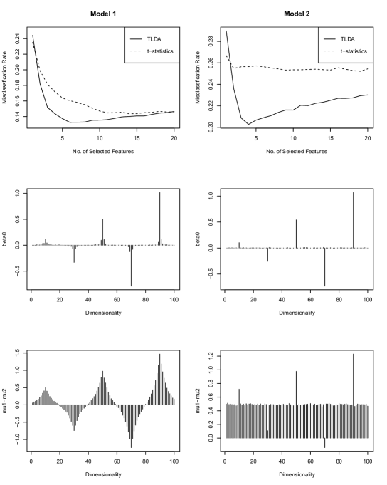
Figure 1: Plots for TLDA and the $t$-statistic. Upper: average misclassification rates versus number of selected features; Middle: average $\beta_{0}$ representing the signal of choosing features by TLDA; Lower: average $\mu_{1}-\mu_{2}$ representing the signal of choosing features by the $t$-statistic.

The figure shows that TLDA always selects more useful features than the two-sample $t$-statistic, which ignores the correlation between features. Specifically, due to correlations, features $30$ and $70$ cannot be detected by the two-sample $t$-statistic for Model 2.

In the second simulation, we study the misclassification rate of our TLDA method. In Cai and Liu (2011) and Fan et al. (2012), the authors have conducted many numerical investigations to compare their methods with others, including the oracle features annealed independence rule (OFAIR) (Fan and Fan, 2008) and nearest shrunken centroid (NSC) method (Tibshirani et al., 2002), and concluded that their methods perform better. We therefore compare TLDA only with LPD and ROAD and do not consider other classic methods. Table 1 shows the misclassification rates based on 100 replications for TLDA, LPD, ROAD, naive Bayes (NB) and Oracle.

Table 1: Average misclassification rates in percentage for sparse situations. Standard deviations are given in parentheses.

$p$	TLDA	LPD	ROAD	NB	Oracle
Model 1
100	13.41(2.68)	13.58(2.48)	16.68(5.44)	16.94(2.64)	11.59(2.18)
200	13.31(2.45)	13.62(2.55)	16.19(5.05)	17.18(2.54)	11.66(2.38)
400	13.99(2.56)	14.06(2.69)	17.45(5.49)	18.86(2.67)	11.88(2.39)
800	14.16(2.94)	14.93(2.96)	18.22(5.08)	20.56(2.92)	11.74(2.30)
Model 2
100	20.78(3.01)	21.04(3.14)	25.01(4.47)	35.13(3.02)	18.41(2.66)
200	20.91(3.26)	21.58(3.27)	25.49(3.91)	35.92(2.76)	18.55(2.55)
400	21.49(3.50)	22.49(3.55)	26.04(3.88)	35.87(2.86)	18.60(2.76)
800	21.99(3.70)	23.31(3.75)	26.62(3.71)	36.04(3.03)	18.70(3.13)

From Table 1, we can see that the performance of TLDA is similar to that of Oracle and is better than that of the other methods. Clearly, due to its fundamental drawback, the naive Bayes is the worst of all methods although it is better than random guess (whose misclassification rate is 50%). Overall, compared with LPD and ROAD, TLDA has the smallest misclassification rate, and the standard deviation of TLDA is similar to that of LPD but smaller than that of ROAD. When the dimensionality $p$ increases from 100 to 800, TLDA is quite stable, whereas LPD and ROAD become increasingly worse. In particular, TLDA always has a smaller misclassification rate and standard deviation than ROAD. When $p$ is not large, TLDA and LPD have similar performance, while TLDA becomes better than LPD as $p$ increases; in particular when $p$ is sufficiently large (such as $p=800$), the difference between the misclassification rates of TLDA and LPD becomes bigger. In summary, simulations demonstrate that TLDA is a stable and superior classification method compared to existing methods.

Next, we will study the estimators $\hat{\beta}_{TLDA},\hat{\beta}_{LPD}$, and $\hat{\beta}_{ROAD}$. Fig. 2 plots the average estimators of 100 replications. Due to different assumptions, here we adjust $\hat{\beta}_{ROAD}$ to $|\beta_{0}|^{2}*\hat{\beta}_{ROAD}$ so that it fits the real situation.

Figure 2: Average estimators of TLDA, LPD and ROAD for $p=100$. The true $\beta_{0}$ and the estimators are very sparse, which is why there is an almost solid line at zero.

From Fig. 2, we can see that TLDA correctly selects most of those five features but very few noise features. In particular, compared with LPD, which estimates the true $\beta_{0}$ directly, our two-stage estimators are much closer to $\beta_{0}$, which is consistent with the discussions in Candes and Tao (2007).

The above simulations are conducted for scenarios where $\beta_{0}$ is sparse. In practice, it is quite common that there are many weak signals that are correlated with the main signals. It would be interesting to evaluate the performance of TLDA for these approximately sparse situations. Specifically, we will consider two scenarios with respect to $\mu_{1}$, as follows.

• Model 3. $\mu_{1}=(1_{5},0_{p-5})$ in Model 1.

• Model 4. $\beta_{0}=0.551*(3,1.7,-2.2,-2.1,2.55,(p-5)^{-1}1_{p-5})$ and $\mu_{1}=\Sigma*\beta_{0}$ in Model 2.

Here $n_{1}=n_{2}=100$ and $\mu_{2}=0$. Model 3 is similar to those in Cai and Liu (2011) and Fan et al. (2012), and Model 4 comes from Mai et al. (2012). The average misclassification rates based on 100 replications are reported in Table 2. It is again evident that TLDA performs favorably compared to existing methods.

Table 2: Average misclassification rates in percentage for approximately sparse simulations. Standard deviations are given in parentheses.

$p$	TLDA	LPD	ROAD	NB	Oracle
Model 3
100	20.70(3.12)	22.69(3.67)	26.85(5.91)	31.46(4.07)	18.56(2.54)
200	20.89(3.11)	24.03(3.83)	27.52(5.37)	33.74(3.68)	18.98(2.65)
400	20.96(3.18)	25.03(3.77)	28.03(5.36)	36.61(3.69)	18.65(2.59)
800	21.75(4.56)	26.77(4.60)	28.73(5.14)	40.71(3.63)	18.80(2.69)
Model 4
100	11.99(2.68)	12.30(2.59)	14.57(3.33)	21.87(2.68)	9.98(2.07)
200	12.64(2.58)	13.04(2.67)	15.15(3.19)	22.17(2.97)	10.60(2.06)
400	12.70(2.64)	13.52(2.40)	15.56(3.09)	22.28(2.79)	10.03(2.17)
800	12.90(3.01)	13.85(2.94)	15.35(3.75)	22.33(3.11)	10.08(2.21)

4 Real data

In this section, we apply the proposed TLDA to real datasets. Since real data usually has an ultra-high data dimension $p$, a sure independence screening (SIS) method (Fan and Lv, 2008) will be carried out before our proposed feature selection procedure to further improve the accuracy and control the computational cost. For brevity, we will apply the two-sample $t$-test statistic (Tibshirani et al., 2002; Fan and Fan, 2008) to reduce the dimensionality from ultra-high to a moderate scale. Other screening steps such as that in Fan et al. (2012) can also be used, but we do not pursue them in detail.

First, TLDA is applied to study leukemia data, which is available at http://www.broadinstitute.org/cgi-bin/cancer/datasets.cgi. The dataset contains $p=7129$ genes for $n_{1}=27$ acute lymphoblastic leukemia (ALL) samples and $n_{2}=11$ acute myeloid leukemia (AML) samples in the training set; the test set consists of 20 ALL samples and 14 AML samples. More details can be found in Golub et al. (1999). By following similar pre-processing steps as Dudoit et al. (2002a) and Fan and Fan (2008), we standardize each sample to zero mean and $S_{n}=\frac{1}{n}\sum_{k=1}^{2}\sum_{j=1}^{n_{k}}(X_{k,j}-\bar{X}_{k})(X_{k,j}-\bar{X}_{k})^{T}$ has unit diagonal elements.

For comparison with LPD in Cai and Liu (2011), we use 2867 genes with the largest absolute values of the two-sample $t$-statistic ($|\mu_{1}-\mu_{2}|>0.5$). Fig. 3 shows the mean difference and estimator $\hat{\beta}_{0}$ (tuning parameter $\lambda=1.2$), representing the feature selection signals of the two-sample $t$-statistic and TLDA, respectively.

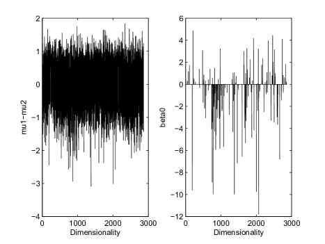
Figure 3: True mean difference and estimator $\hat{\beta}_{0}$ of leukemia data.

Clearly, the signal for TLDA is sparse, while the signal for the two-sample $t$-statistic has no clear clues. The classification results for TLDA, LPD, ROAD, OFAIR, NSC, and NB are shown in Table 3.

Table 3: Classification errors of leukemia data by various methods

	TLDA	LPD	ROAD	OFAIR	NSC	NB
Training Error	0/38	0/38	0/38	1/38	1/38	0/38
Test Error	1/34	1/34	1/34	1/34	3/34	5/34
No. of Selected genes	8	151	40	11	24	7129

Table 3 shows that TLDA performs competitively in classification error with LPD and ROAD. However, TLDA only selects 8 genes, in contrast to 40 genes by ROAD and 151 genes by LPD. The 8 selected genes and their TLDA weights are given in Table 4. For comparison, we also present their $t$-statistic rank in the 7129 genes.

Table 4: The eight genes of leukemia data selected by TLDA.

Gene position		TLDA weights		Rank of $t$-statistic
461		-3.203		7
1779		-4.455		87
1834		-5.039		6
3320		-0.960		1
3525		-3.876		138
4847		-6.389		2
5039		-1.187		4
6539		-7.9933		21

We further compare the methods on two more real datasets: the colon (Srivastava and Kubokawa, 2007) and breast cancer (Hess et al., 2006) datasets. A leave-one-out cross validation (LOOCV) is performed on the two datasets. For $i=1,\cdots,n$ , the $p\times 1$ vector $x_{i}$ is treated as the testing set, while the remaining $n-1$ observations form the training set. A subset of 1000 genes is selected based on the two-sample t-statistic. The classification results for the TLDA, LPD, ROAD, and NB methods are shown in Table 5. We can see that, on each dataset, the proposed TLDA has a competitive performance in terms of classification errors while using the fewest genes. Overall, TLDA is also applicable in real datasets and performs favorably in comparison to existing methods.

Table 5: Classification error and number of genes selected by various methods for the colon and breast cancer datasets

		TLDA	LPD	ROAD	NB
Colon	Error(%)	9.68	9.68	11.29	14.52
	No. of genes	7.42(1.03)	168.95(71.39)	38.10(27.60)	1000(0)
Breast	Error(%)	21.80	25.56	31.58	34.59
	No. of genes	14.61(2.40)	332.45(103.56)	44.14(47.26)	1000(0)

5 Discussions

In this paper, we have proposed a solution for feature selection in high-dimensional data. We have derived the optimal feature selection rule for LDA and proposed the selection of features based on the sparsity of $\Sigma^{-1}\mu_{d}$. An $l_{1}$ minimization method is used on the samples to select the important features and LDA is then applied to those selected features. Our proposed TLDA performs favorably compared to existing methods in theory and application. Our analysis shows that the independent rules such as the two-sample $t$-statistic and naive Bayes may not be efficient and may even lead to bad classifiers.

Suppose that there are $K>2$ classes (in this article we assume that $K=2$), our TLDA is also applicable. For this, $X$ will be classified to class $k$ if and only if

$$(X-(\bar{X}_{k}+\bar{X}_{l})/2)_{\mathcal{A}_{kl}^{\ast}}^{T}\beta_{kl}^{\ast}>0~{}for~{}all~{}k\neq l.$$ (5.10)

Moreover, the procedure can be extended to unequal prior probabilities $\pi_{1}$ and $\pi_{2}$ in which we classify $X$ to class 1 when

$$(X-(\bar{X}_{1}+\bar{X}_{2})/2)_{\mathcal{A}^{\ast}}^{T}\beta^{\ast}>\log{(\pi_{2}/\pi_{1})},$$ (5.11)

where the parameters can also be estimated as $\hat{\pi}_{1}=n_{1}/n$ and $\hat{\pi}_{2}=n_{2}/n$. For non-Gaussian distributions, we can also derive similar results under the moment conditions, as in Cai and Liu (2011).

Finally, we note that the number of selected features is $p_{0}=o(\sqrt{n/\log{p}})$ which is very small compared to $p$. Setting $n=O((\log{p})^{\beta})$ for $\beta>1$, this means that only $o((\log{p})^{(\beta-1)/2})$ features can be selected from $p$ variables to apply LDA. This is due to the fact that LDA is stable only when $p_{0}\sqrt{p_{0}/n}\to 0$, and a detailed result can be found in Shao et al. (2011). Our future research will focus on improving $p_{0}$.

Appendix A: Proofs

A.1. Proof of Theorem 2.1

From the proofs of Theorem 2 in Cai and Liu (2011), we know that

$$(\hat{\beta}-\beta_{0})^{T}\Sigma(\hat{\beta}-\beta_{0})\leq C|\beta_{0}|_{1}^{2}\sqrt{\log{p}/n}+6\lambda_{n}|\beta_{0}|_{1},$$ (5.12)

with probability greater than $1-O(p^{-1})$. Using the Cauchy-Schwartz inequality,

$$|\beta_{0}|_{1}^{2}\leq|\beta_{0}|_{0}|\beta_{0}|_{2}^{2}\leq c_{0}p_{0}(\beta_{0}^{T}\Sigma\beta_{0})=4c_{0}p_{0}\Delta_{p},$$

$$(\hat{\beta}-\beta_{0})^{T}\Sigma(\hat{\beta}-\beta_{0})\geq c_{0}^{-1}(\hat{\beta}-\beta_{0})^{T}(\hat{\beta}-\beta_{0}).$$

Together with (5.12), we have

$$(\hat{\beta}-\beta_{0})^{T}(\hat{\beta}-\beta_{0})\leq Cp_{0}\Delta_{p}\sqrt{\log{p}/n},$$ (5.13)

with probability greater than $1-O(p^{-1})$. For $j\in\mathcal{A}$,

$$|\hat{\beta}_{j}-(\beta_{0})_{j}|^{2}\leq Cp_{0}\Delta_{p}\sqrt{\log{p}/n}.$$

Then

$$|\hat{\beta}_{j}| \geq |(\beta_{0})_{j}|-\sqrt{Cp_{0}\Delta_{p}\sqrt{\log{p}/n}}$$

$$\geq c_{p}(1-\sqrt{Cp_{0}\Delta_{p}\sqrt{\log{p}/n}}/c_{p})$$

$$> c_{p}/2.$$

Similarly, for $j\in\mathcal{A}^{c}$,

$$|\hat{\beta}_{j}|\leq\sqrt{Cp_{0}\Delta_{p}\sqrt{\log{p}/n}}<c_{p}/2.$$

Hence, we have proved that $P(\mathcal{A}^{\ast}=\mathcal{A})=1-O(p^{-1})$.

A.2. Proof of Theorem 2.2

Applying the features selector $\mathcal{A}^{\ast}$ to the sample $\{X_{1,j},j=1,\cdots,n_{1}\}$ and $\{X_{2,j},j=1,\cdots,n_{2}\}$, we still denote the corresponding data as $X,\{X_{k,j},k=1,2\}$ for brevity. It is noted that here the dimension is $p_{0}$ not $p$. Setting

$$\bar{X}_{k}=\frac{1}{n_{k}}\sum_{j=1}^{n_{k}}X_{1,j},~{}~{}k=1,2,$$

$$S_{n}=\frac{1}{n}\sum_{k=1}^{2}\sum_{j=1}^{n_{k}}(X_{k,j}-\bar{X}_{k})(X_{k,j}-\bar{X}_{k})^{T},$$

and

$$\hat{\mu}_{a}=\frac{\bar{X}_{1}+\bar{X}_{2}}{2},~{}\hat{\mu}_{d}=\frac{\bar{X}_{1}-\bar{X}_{2}}{2}.$$

The LDA procedure is

$$\delta_{LDA}(X)=I\{(X-\hat{\mu}_{a})^{T}S_{n}^{-1}\hat{\mu}_{d}\},$$

and the misclassification rate is

$$R_{\mathcal{A}^{\ast}}=\frac{1}{2}\Phi(\frac{(\hat{\mu}_{a}-\mu_{1})S_{n}^{-1}\hat{\mu}_{d}}{(\hat{\mu}_{d}^{T}S_{n}^{-1}\Sigma S_{n}^{-1}\hat{\mu}_{d})^{1/2}})+\frac{1}{2}\Phi(-\frac{(\hat{\mu}_{a}-\mu_{2})S_{n}^{-1}\hat{\mu}_{d}}{(\hat{\mu}_{d}^{T}S_{n}^{-1}\Sigma S_{n}^{-1}\hat{\mu}_{d})^{1/2}}).$$

By the proofs of Theorem 1 in Shao et al. (2011), we know that

$$\frac{(\hat{\mu}_{a}-\mu_{1})S_{n}^{-1}\hat{\mu}_{d}}{(\hat{\mu}_{d}^{T}S_{n}^{-1}\Sigma S_{n}^{-1}\hat{\mu}_{d})^{1/2}}=-\Delta_{p}^{1/2}(1+O(p_{0}\sqrt{\log{p_{0}}/n})),$$

and a similar result also holds for $\Phi(\frac{(\hat{\mu}_{a}-\mu_{1})S_{n}^{-1}\hat{\mu}_{d}}{(\hat{\mu}_{d}^{T}S_{n}^{-1}\Sigma S_{n}^{-1}\hat{\mu}_{d})^{1/2}})$. Then

$$R_{\mathcal{A}^{\ast}}=\Phi(-\Delta_{p}^{1/2}(1+O(p_{0}\sqrt{\log{p_{0}}/n}))).$$ (5.14)

Noting that $p_{0}\sqrt{\log{p_{0}}/n}\to 0$, therefore, in probability,

$$R_{\mathcal{A}^{\ast}}-R\to 0.$$ (5.15)

From equation (12) of Cai and Liu (2011), we know that

$$|\frac{\Phi(\frac{(\hat{\mu}_{a}-\mu_{1})S_{n}^{-1}\hat{\mu}_{d}}{(\hat{\mu}_{d}^{T}S_{n}^{-1}\Sigma S_{n}^{-1}\hat{\mu}_{d})^{1/2}})}{\Phi(-\Delta_{p}^{1/2})}-1|\leq O(\Delta_{p}p_{0}\sqrt{\log{p_{0}}/n})e^{O(\Delta_{p}p_{0}\sqrt{\log{p_{0}}/n})}.$$

Then

$$|\frac{R_{\mathcal{A}^{\ast}}}{R}-1|\leq O(\Delta_{p}p_{0}\sqrt{\log{p_{0}}/n})e^{O(\Delta_{p}p_{0}\sqrt{\log{p_{0}}/n})}.$$

When $\Delta_{p}p_{0}\sqrt{\log{p_{0}}/n}\to 0$, we get

$$|\frac{R_{\mathcal{A}^{\ast}}}{R}-1|=O(\Delta_{p}p_{0}\sqrt{\log{p_{0}}/n}).$$ (5.16)

The proof is completed.

References

- Anderson (2003) Anderson, T., 2003. An introduction to multivariate statistical analysis (3rd ed.). Wiley-Interscience, New Jersey.
- Barry et al. (2005) Barry, W., Nobel, A., Wright, F., 2005. Significance analysis of functional categories in gene expression studies: a structured permutation approach. Bioinformatics 21 (9), 1943–1949.
- Bickel and Levina (2004) Bickel, P., Levina, E., 2004. Some theory for Fisher’s linear discriminant function, naive Bayes’, and some alternatives when there are many more variables than observations. Bernoulli 10 (6), 989–1010.
- Cai and Liu (2011) Cai, T., Liu, W., 2011. A direct estimation approach to sparse linear discriminant analysis. Journal of the American Statistical Association 106 (496), 1566–1577.
- Candes and Tao (2007) Candes, E., Tao, T., 2007. The Dantzig selector: statistical estimation when p is much larger than n. The Annals of Statistics 35 (6), 2313–2351.
- Donoho et al. (2006) Donoho, D., Elad, M., Temlyakov, V., 2006. Stable recovery of sparse overcomplete representations in the presence of noise. IEEE Transactions on Information Theory 52 (1), 6–18.
- Dudoit et al. (2002a) Dudoit, S., Fridlyand, J., Speed, T., 2002a. Comparison of discrimination methods for the classification of tumors using gene expression data. Journal of the American Statistical Association 97 (457), 77–87.
- Dudoit et al. (2002b) Dudoit, S., Yang, Y., Callow, M., Speed, T., 2002b. Statistical methods for identifying differentially expressed genes in replicated CDNA microarray experiments. Statistica Sinica 12 (1), 111–140.
- Fan and Fan (2008) Fan, J., Fan, Y., 2008. High dimensional classification using features annealed independence rules. The Annals of Statistics 36 (6), 2605.
- Fan et al. (2012) Fan, J., Feng, Y., Tong, X., 2012. A road to classification in high dimensional space. Journal of the Royal Statistical Society. Series B, Statistical methodology 74 (4), 745.
- Fan and Lv (2008) Fan, J., Lv, J., 2008. Sure independence screening for ultrahigh dimensional feature space. Journal of the Royal Statistical Society: Series B (Statistical Methodology) 70 (5), 849–911.
- Goeman et al. (2004) Goeman, J., Van De Geer, S., De Kort, F., Van Houwelingen, H., 2004. A global test for groups of genes: testing association with a clinical outcome. Bioinformatics 20 (1), 93.
- Golub et al. (1999) Golub, T., Slonim, D., Tamayo, P., Huard, C., Gaasenbeek, M., Mesirov, J., Coller, H., Loh, M., Downing, J., Caligiuri, M., et al., 1999. Molecular classification of cancer: class discovery and class prediction by gene expression monitoring. Science 286 (5439), 531.
- Hess et al. (2006) Hess, K., Anderson, K., Symmans, W., Valero, V., Ibrahim, N., Mejia, J., Booser, D., Theriault, R., Buzdar, A., Dempsey, P., et al., 2006. Pharmacogenomic predictor of sensitivity to preoperative chemotherapy with paclitaxel and fluorouracil, doxorubicin, and cyclophosphamide in breast cancer. Journal of Clinical Oncology 24 (26), 4236–4244.
- Lai (2008) Lai, Y., 2008. Genome-wide co-expression based prediction of differential expressions. Bioinformatics 24 (5), 666–673.
- Li et al. (2001) Li, L., Weinberg, C., Darden, T., Pedersen, L., 2001. Gene selection for sample classification based on gene expression data: study of sensitivity to choice of parameters of the GA/KNN method. Bioinformatics 17 (12), 1131.
- Mai et al. (2012) Mai, Q., Zou, H., Yuan, M., 2012. A direct approach to sparse discriminant analysis in ultra-high dimensions. Biometrika 99 (1), 29–42.
- Shao et al. (2011) Shao, J., Wang, Y., Deng, X., Wang, S., 2011. Sparse linear discriminant analysis by thresholding for high dimensional data. The Annals of Statistics 39 (2), 1241–1265.
- Srivastava and Kubokawa (2007) Srivastava, M., Kubokawa, T., 2007. Comparison of discrimination methods for high dimensional data. Journal of the Japan Statistical Society 37 (1), 123–134.
- Tibshirani et al. (2002) Tibshirani, R., Hastie, T., Narasimhan, B., Chu, G., 2002. Diagnosis of multiple cancer types by shrunken centroids of gene expression. Proceedings of the National Academy of Sciences 99 (10), 6567.
- Tibshirani and Wasserman (2006) Tibshirani, R., Wasserman, L., 2006. Correlation-sharing for detection of differential gene expression. Arxiv preprint math/0608061.
- Tong et al. (2012) Tong, T., Chen, L., Zhao, H., 2012. Improved mean estimation and its application to diagonal discriminant analysis. Bioinformatics 28 (4), 531–537.
- Wu et al. (2009) Wu, M., Zhang, L., Wang, Z., Christiani, D., Lin, X., 2009. Sparse linear discriminant analysis for simultaneous testing for the significance of a gene set/pathway and gene selection. Bioinformatics 25 (9), 1145.
- Yeung et al. (2012) Yeung, K., Gooley, T., Zhang, A., Raftery, A., Radich, J., Oehler, V., 2012. Predicting relapse prior to transplantation in chronic myeloid leukemia by integrating expert knowledge and expression data. Bioinformatics 28 (6), 823.
- Zuber and Strimmer (2009) Zuber, V., Strimmer, K., 2009. Gene ranking and biomarker discovery under correlation. Bioinformatics 25 (20), 2700–2707.