The energy of waves in the photosphere and lower chromosphere: II. Intensity statistics

Abstract

Context. The energy source that maintains the solar chromosphere is still undetermined, but leaves its traces in observed intensities.

Aims. We investigate the statistics of the intensity distributions as function of the wavelength for Ca ii H and the Ca ii IR line at 854.2 nm to estimate the energy content in the observed intensity fluctuations.

Methods. We derived the intensity variations at different heights of the solar atmosphere as given by the line wings and line cores of the two spectral lines. We converted the observed intensities to absolute energy units employing reference profiles calculated in non-local thermal equilibrium (NLTE). We also converted the observed intensity fluctuations to corresponding brightness temperatures assuming LTE.

Results. The root-mean-square (rms) fluctuations of the emitted intensity are about 0.6 (1.2) Wm^-2ster^-1pm^-1 near the core of the Ca ii IR line at 854.2 nm (Ca ii H), corresponding to relative intensity fluctuations of about 20 % (30 %). Maximum fluctuations can be up to 400 %. For the line wing, we find rms values of about 0.3 Wm^-2ster^-1pm^-1 for both lines, corresponding to relative fluctuations below 5 %. The relative rms values show a local minimum for wavelengths forming at about 130 km height, but otherwise increase smoothly from the wing to the core, i.e., from photosphere to chromosphere. The corresponding rms brightness temperature fluctuations are below 100 K for the photosphere and up to 500 K in the chromosphere. The skewness of the intensity distributions is close to zero in the outer line wing and positive throughout the rest of the line spectrum, caused by a frequent occurrence of high-intensity events. The skewness shows a pronounced local maximum on locations with photospheric magnetic fields for wavelengths in between the line wing and the line core ($z\approx\,150-300$ km), and a global maximum at the very core ($z\approx\,1000$ km) for both magnetic and field-free locations.

Conclusions. The energy content of the intensity fluctuations is insufficient to create a similar temperature rise in the chromosphere as predicted in most reference models of the solar atmosphere. The increase of the rms fluctuations with height indicates the presence of upwards propagating acoustic waves with an increasing oscillation amplitude. The intensity and temperature variations show a clear increase of the dynamics from photosphere towards the chromosphere, but fall short of fully dynamical chromospheric models by a factor of about five. The enhanced skewness between photosphere and lower solar chromosphere on magnetic locations indicates a mechanism which solely acts on magnetized plasma. Possible candidates are the Wilson depression, wave absorption, or magnetic reconnection.

1 Introduction

The solar chromosphere shows prominent emission lines when viewed near the solar limb, e.g., during an eclipse, but also on the solar disc chromospheric spectral lines such as H$\alpha$, Ca ii H and K, Mg ii h and k, or the Ca ii IR triplet revert to transient emission. Because the gas density is so low that the material is transparent and the radiation temperature is decreasing above the continuum forming layers in the photosphere, the emission lines require an energy supply other than radiative transfer. The different types of possible heating mechanisms vary from purely mechanical processes to all processes that can be related to the presence of magnetic field lines (see, e.g., Biermann 1948; Schatzman 1949; Liu 1974; Anderson & Athay 1989; Davila & Chitre 1991; Rammacher & Ulmschneider 1992; Narain & Ulmschneider 1996; Carlsson et al. 2007; Rezaei et al. 2007a; Beck et al. 2008; Fontenla et al. 2008; Beck et al. 2009; Khomenko & Collados 2012).

In addition to the fact that “the” heating mechanism of the chromosphere could not be identified yet, the exact amount of energy required to maintain the chromosphere as it is observed is not fully clear. There exists a series of static atmospheric stratification models for the solar photosphere and chromosphere (e.g., Gingerich et al. 1971; Vernazza et al. 1976, 1981; Fontenla et al. 2006; Avrett & Loeser 2008) that were determined from temporally and/or spatially averaged spectra. These models mainly share the existence of a temperature reversal at a certain height in the solar atmosphere, the location of the temperature minimum. Using temporally and spatially resolved spectra, it seems that the assumption of a static background temperature with minor variation around it is not fulfilled (e.g., Liu & Skumanich 1974; Kalkofen et al. 1999; Carlsson & Stein 1997; Rezaei et al. 2008). The spectra indicate in some cases that no chromospheric temperature rise is present at all (Liu & Smith 1972; Cram & Dame 1983; Rezaei et al. 2008), as is also required by the observations of CO molecular lines in the lower chromosphere (Ayres & Testerman 1981; Ayres 2002) that only form at temperatures below about 4000 K. Numerical hydrodynamical (HD) simulations of the chromosphere show even lower temperatures down to 2000 K (Wedemeyer-Böhm et al. 2004; Leenaarts et al. 2011).

In the first paper of this series (Beck et al. 2009, BE09) we investigated the energy content of velocity oscillations in several photospheric spectral lines and the chromospheric Ca ii H line. The main finding of BE09 was that the energy of the root-mean-square (rms) velocity of a spectral line in the wing of Ca ii H, whose formation height was estimated to be about 600 km, was already below the chromospheric energy requirement of 4.3 kWm^-2 given by Vernazza et al. (1976), with a further decrease of the energy content towards higher layers. The observations used had a spatial resolution of about 1^′′, similar to those of Fossum & Carlsson (2005, 2006) that also found an insufficient energy in intensity oscillations observed with TRACE. Wedemeyer-Böhm et al. (2007) and Kalkofen (2007) demonstrated later that the spatial resolution can be critical for the determination of the energy content, because the spatial smearing hides high-frequency oscillations with their corresponding short wavelengths.

Recently, several papers addressed the energy flux of acoustic and gravity waves using data of higher spatial resolution from, e.g., the Göttingen Fabry-Perot Interferometer (GFPI, Puschmann et al. 2006), the Interferometric BI-dimensional Spectrometer (IBIS, Cavallini 2006), or the Imaging Magnetograph eXperiment (IMaX) onboard of the Sunrise balloon mission (Jochum et al. 2003; Gandorfer et al. 2006; Martínez Pillet et al. 2011). Straus et al. (2008) found an energy flux of solar gravity waves of 5 kWm^-2 at the base of the chromosphere in simulations and observations, usually an order of magnitude higher than the energy flux of acoustic waves at the same height. Bello González et al. (2009, 2010) found an acoustic energy flux of 3 and $>$ 6 kWm^-2 at a height of 250 km, using GFPI and IMaX data, respectively (see also Table 2 in Bello González et al. 2010). Much of the wave energy was found in the frequency range above the acoustic cut-off frequency of about 5 mHz; these high-frequency waves are able to propagate into the chromosphere without strong (radiative) losses (cf. also Carlsson & Stein 2002; Reardon et al. 2008). The energy content was, however, basically determined from photospheric spectral lines, and thus refers to the upper photosphere, where also at lower spatial resolution sufficient mechanical energy is seen (BE09). Interestingly, the (lower) chromospheric lines used in Straus et al. (2008), Na i D and Mg i $b_{2}$, showed an energy flux below 4 kWm^-2 (their Fig. 3). It is therefore unclear how reliable the extrapolation of the photospheric energy fluxes actually is.

Another point to be considered is the influence of the photospheric magnetic fields on the chromospheric behaviour (e.g., Cauzzi et al. 2008). Photospheric magnetic fields also cause an enhancement of the chromospheric emission, even if the underlying process may be a kind of wave propagation in the end (e.g., Hasan 2000; Rezaei et al. 2007a; Beck et al. 2008; Hasan & van Ballegooijen 2008; Khomenko et al. 2008; Vigeesh et al. 2009; Fedun et al. 2011). The usage of velocity oscillations to estimate the energy content is in general also less direct than to use the intensity spectrum. If energy is deposited into the upper solar atmosphere by a process without a clear observable signature, either because of missing spatial or temporal resolution, or because of physical reasons such as for the case of transversal wave modes, the emitted intensity will still react to the energy deposit, even if the non-local thermal equilibrium (NLTE) conditions in the chromosphere make the reaction neither instantaneous nor necessarily linear to the amount of deposited energy. For instance, Reardon et al. (2008) found evidence that the passage of shock fronts induces turbulent motions at chromospheric heights. The dissipation of the energy of these turbulent motions then would effect an energy transfer from mechanical to radiative energy, but with some time delay and over some period longer than the duration of the shock passage itself (see also Verdini et al. 2012).

In this contribution, we investigate the intensity statistics of two chromospheric spectral lines, Ca ii H and the Ca ii IR line at 854.2 nm, to estimate the energy contained in their intensity variations at all wavelengths from the wing to the very line core. Section 2 describes the observations used. The data reduction steps are detailed in Sect. 3. In Sect. 4, we investigate the intensity statistics of the two lines. The results are summarized and discussed in Sect. 5, whereas Sect. 6 provides our conclusions.

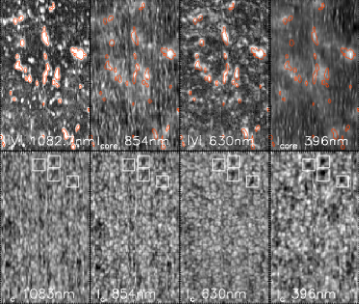
Observation No. 3     Observation No. 4

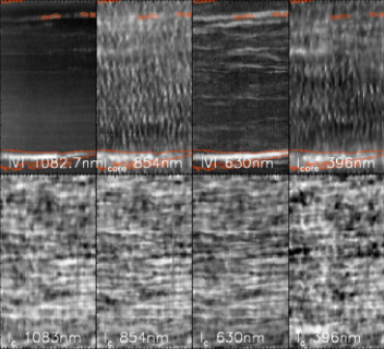
Figure 1: Overview maps of the observation No. 3 (left panel) and No. 4 (right panel). Bottom row, left to right: continuum intensity at 1083 nm, 854 nm, 630 nm, and 396 nm. Top row, left to right: unsigned wavelength-integrated Stokes $V$ signal around Si i at 1082.7 nm, line-core intensity of the Ca ii IR line at 854.2 nm, unsigned wavelength-integrated Stokes $V$ signal around 630 nm, line-core intensity of Ca ii H at 396.85 nm. The red contours outline strong polarisation signals. The white squares denote co-spatial local darkenings.

Table 1: Overview of the observations.

No.	date	type	$t_{\rm int}$	size	Ca ii IR
1	24/07/06	map	6.6 sec	75${}^{\prime\prime}\times 70^{\prime\prime}$	no
2	24/07/06	time series	3.3 sec	60 min	no
3	29/08/09	map	$\sim 30$  sec	40${}^{\prime\prime}\times 70^{\prime\prime}$	yes
4	08/09/09	time series	5 sec	50 min	yes

2 Observations

We used four different observations, two large-area maps and two time series of about one hour duration, all observed in quiet Sun (QS) on disc centre with real-time seeing correction by the Kiepenheuer-Institute Adaptive Optics System (KAOS, von der Lühe et al. 2003). One of the large-area maps and one time series were taken in the morning of 24 July 2006. They are already described in detail in Beck et al. (2008, BE08) and BE09; we thus only shortly summarize their characteristics. The large-area map covered an area of 75${}^{\prime\prime}\times$ 70^′′, taken by moving the 0$\aas@@fstack{\prime\prime}$5 wide slit of the POlarimetric LIttrow Spectrograph (POLIS, Beck et al. 2005c) at the German Vacuum Tower Telescope (VTT, Schröter et al. 1985) in steps of 0$\aas@@fstack{\prime\prime}$5 across the solar image. For the time series, the cadence of co-spatial positions was about 21 seconds. POLIS provided the Stokes vector around 630 nm together with intensity profiles of Ca ii H. The spatial sampling along the slit was 0$\aas@@fstack{\prime\prime}$29 for Ca ii H and half of that for 630 nm. The polarimetric data at 630 nm were calibrated with the methods described in Beck et al. (2005c, b). These observations will be labeled No. 1 (large-area map on 24 July 2006) and No. 2 (times series on 24 July 2006) in the following; Table 1 lists additionally the integration time $t_{\rm int}$ per scan step.

The third observation is another large-area map on disc centre from 28 August 2009, UT 08:33:42 until 09:42:08, this time taken simultaneously with POLIS, the Tenerife Infrared Polarimeter (TIP, Martínez Pillet et al. 1999; Collados et al. 2007), and a PCO 4000 camera on the output port of the main spectrograph of the VTT to record spectra of the Ca ii IR line at 854.2 nm . TIP observed the wavelength range around 1083 nm, including a photospheric Si i line at 1082.7 nm and the chromospheric He i line at 1083 nm. The slit width of the main spectrograph was 0$\aas@@fstack{\prime\prime}$36 and the spatial sampling along the slit was 0$\aas@@fstack{\prime\prime}$17 for both TIP and the Ca ii IR camera. The spectral sampling of Ca ii IR was 1.6 pm per pixel, after a binning by two in wavelength to increase the light level. The step width was 0$\aas@@fstack{\prime\prime}$35 for all instruments in this case, and the slit width and spatial sampling for POLIS were the same as given above for observations Nos. 1 and 2. The integration time per scan step was 30 seconds for TIP and 26 seconds for POLIS, allowing us to observe also the weakest polarisation signals belonging to the weak magnetic fields in the internetwork of the QS because of the high signal-to-noise (S/N) ratio of the data. The rms noise of the polarisation signal at continuum wavelengths was about 3$\cdot 10^{-4}$ of the continuum intensity $I_{c}$ at 630 nm and 4.3$\cdot 10^{-4}$ of $I_{c}$ for TIP at 1083 nm.

The PCO 4000 camera for the Ca ii IR spectra was triggered by TIP at the start of each scan step and used an exposure time of 25 seconds, slightly shorter than the integration time for TIP and POLIS. The spectra of Ca ii IR were taken through the polarimeter of TIP, including the separation into two orthogonally polarised beams. In the data reduction, the two beams in Ca ii IR were only cut out from the image and added, because without the synchronization to the polarisation modulation of TIP only intensity spectra can be obtained. This observation will be referred to as No. 3 in the following. The wavelength range in Ca ii IR extended from about 853.3 nm up to 854.8 nm thanks to the large CCD size (compare to the range commonly used in IBIS, e.g., Cauzzi et al. 2008).

With the same setup, a time series of about 50 minutes duration was obtained on 8 September 2009 between UT 08:07:40 and 08:58:59 (observation No. 4). The integration time per scan step was 5 seconds and the observation consisted of 112 repeated scans of four steps of 0$\aas@@fstack{\prime\prime}$5 step width each. Only one of the four scan steps from the TIP and POLIS data was co-spatial in all wavelengths (396 nm, 630 nm, 854 nm, 1083 nm) because of the differential refraction in the Earths’ atmosphere (Reardon 2006; Beck et al. 2008) that was (partly) compensated by intentionally displacing the two slits of POLIS and TIP (see Felipe et al. 2010). We therefore used only the co-spatial scan step that was observed with a cadence of about 27 seconds.

Figure 1 shows overview maps of the observations Nos. 3 and 4, derived from the spectra after the data reduction steps described in the next section. The data have only been aligned with pixel accuracy ($\sim 0\aas@@fstack{\prime\prime}36$), because a better alignment is not critical for the present investigation and is also difficult to achieve for observation No. 3 with its long integration time per scan step. For observation No. 3 (left panel), most of the individual features can be identified in each wavelength range, i.e., the strong polarisation signals of the photospheric Si i line at 1082.7 nm (top left) match those of the Fe i lines at 630 nm (third column in the top row) and also the emission in both chromospheric Ca ii lines matches (second and fourth column in the top row). In the maps of the continuum intensity $I_{c}$ in the bottom row, common features are more difficult to detect, but going from one wavelength to the next allows one to re-encounter some of them. The most prominent examples are four roundish darkenings, seen best at 630 nm and 396 nm (white squares in the $I_{c}$ maps). These darkenings re-appear in the near-IR wavelengths as well, with reduced contrast and slightly displaced. The corresponding maps of observation No. 4 are shown at the right-hand side of Fig. 1. The maps of the continuum intensity in the lower row match well to each other in this case, e.g., compare the locations of the roundish darkenings around $(t,y)=(45\,{\rm min},40^{\prime\prime})$.

3 Additional data reduction steps

3.1 Stray light correction for Ca ii H

In a recent study (Beck et al. 2011, BE11), we investigated the stray light contamination in POLIS. It turned out that for the Ca ii H channel two contributions are important: spectrally undispersed stray light of about 5 % of amplitude created by scattering inside POLIS and spectrally dispersed spatial stray light of about 20 % amplitude. Following the procedure outlined in BE11, we corrected the Ca ii H spectra of POLIS for these two stray light contributions, using a single stray light profile averaged over the full FOV. We subtracted first 5 % of the intensity in the line wing from all wavelengths and subsequently 20 % of the average profile from each individual profile in the observed FOV.

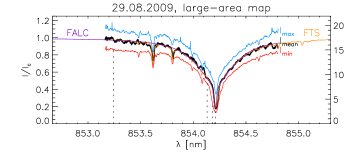
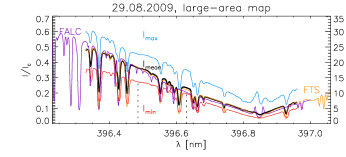
Figure 2: Average observed spectra from the observation No. 3 in comparison to the FTS atlas (orange) and a synthetic FALC NLTE spectrum (purple). Top: Ca ii IR at 854 nm. Bottom: Ca ii H at 396 nm. Black lines: observed average profile. Red/blue: minimum/maximum observed intensity at any wavelength. The vertical dotted lines indicate the wavelengths used as examples later on.

3.2 Intensity normalization

For 630 nm, Ca ii IR, and the TIP spectra, the intensity normalization presents no problems because the observations were done on disc centre and the spectral range covers continuum wavelength ranges. These spectra therefore can be normalized to the continuum intensity, and can then be directly compared to other theoretical or observed reference profiles.

For the Ca ii H spectra, no true continuum wavelengths exist inside the observed spectral range. We thus used a (pseudo)continuum wavelength around 396.5 nm for the normalization. We first determined the normalization coefficient that brought the average observed spectrum on that of the FTS atlas (Kurucz et al. 1984; Neckel 1999). To obtain an absolute intensity scale, we then synthesized Ca ii H and Ca ii IR spectra from the FALC atmosphere stratification (Fontenla et al. 2006) with the NLTE code of Uitenbroek (2001). The intensity of the NLTE profile is given in units of radiated energy per area, time, solid angle, and frequency interval and can be normalized to its “continuum intensity” using spectral windows without strong line blends far to the red and blue of the Ca ii H line core.

Figure 2 shows the final match of the average observed profiles of Ca ii H and the Ca ii IR line at 854.2 nm in observation No. 3, the corresponding section of the FTS atlas, and the FALC NLTE spectrum in both relative intensities $I/I_{c}$ (scale at left) and absolute energy units (scale at right). The corresponding profiles of observations Nos. 1, 2, and 4 are displayed in Fig. 10 in Appendix A. The shape of the lines is nearly identical in all average profiles but for the very line core of Ca ii H that shows some variation between the different observations. This ensures that the conversion from the observed intensity in detector counts to the absolute intensity provided by the synthetic NLTE profile is reliable across different observations. In the following, we will usually denote the intensity as fraction of $I_{c}$; the conversion coefficient is 17.4 Wm^-2ster^-1pm^-1 ($\equiv I_{c}=1$) at 854 nm (cf. Leenaarts et al. 2009, their Fig. 1 yields about 17.3 Wm^-2ster^-1pm^-1) and 50.1 Wm^-2ster^-1pm^-1 at 396 nm.

For each observation, we also overplotted the profiles corresponding to the maximum and minimum intensity observed at each wavelength. These profiles delimit the range of observed intensity variations, but do not correspond to an individual observed profile. For the four observations of Ca ii H, the range of variation is very similar, about $\pm(0.1$ – 0.2) of $I_{c}$ around the average intensity; for the Ca ii IR line at 854.2 nm, the range is about $\pm 0.15$ of $I_{c}$.

Because all average profiles were found to be quite similar, we decided to average all quantities and statistics over all available observations, i.e., all four for Ca ii H and observations Nos. 3 and 4 for the Ca ii IR line at 854.2 nm.

3.3 Polarisation masks

For all observations, simultaneous polarimetric data are available, either in the two Fe i lines at 630 nm (all observations) or in the Si i line at 1082.7 nm (observations Nos. 3 and 4). We defined masks delimiting locations with significant polarisation amplitude in the maps of the wavelength-integrated unsigned Stokes $V$ signal (for examples see Beck & Rammacher 2010, their Appendix A). The threshold was lower than the one used in Fig. 1 where only the strongest polarisation signals are marked. With the masks, in each observed FOV three samples were defined: all locations with significant photospheric polarisation signal (“magnetic”), all locations without significant polarisation signal (“field-free”), and the full FOV. The magnetic sample covered about 10 – 20 % of the total FOV.

4 Intensity statistics

For the intensity statistics, we derived the distributions of intensities as function of the wavelength for the three samples inside the FOV defined above. We then determined the characteristic quantities of the intensity distributions up to second order (average value, standard deviation, skewness of distribution).

4.1 Average profiles $I(\lambda)$

Average profiles of Ca ii H are discussed in detail in BE08. We thus refer the reader to the latter publication, and only summarize their findings here. The average profile of Ca ii H for both field-free and magnetic locations shows an asymmetric emission pattern near the line core, with stronger emission in the H_2V emission peak to the blue of the core at about 396.83 nm than in H_2R to the red at about 396.87 nm (see Fig. 17 in BE08). The asymmetry of the two emission peaks is the signature of upwards propagating shock waves. In the most quiet parts of the FOV, the average profile shows a nearly reversal-free shape without emission as discussed in Rezaei et al. (2008). The average profile of magnetic locations differs from that of the field-free locations by an additional contribution to the emission that is roughly symmetric around the very line core. This contribution presumably indicates a chromospheric heating process that has no counterpart in a Doppler shift of the line in observations on disc centre (e.g, magnetic reconnection with horizontal outflows or transversal wave modes).

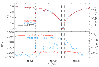
Figure 3: Average profiles of Ca ii IR at 854 nm. Top: average profiles of the full FOV (black), field-free (red) and magnetic locations (blue). Bottom: difference of the profiles of the full FOV and the field-free locations (red solid) and difference of magnetic and field-free locations (blue dash-dotted). The dotted vertical lines denote the locations of line blends, the dashed vertical lines an asymmetry in the intensity differences.

Whereas the shape of the Ca ii H line core changes by a few percent of $I_{c}$ between the different samples (full FOV, magnetic and field-free locations), the variability of the Ca ii IR line at 854.2 nm is smaller (Fig. 3). For the average profiles, one cannot really distinguish between the magnetic locations, the field-free locations, or the full FOV (upper panel of Fig. 3). Subtracting the average profile of the field-free locations as the first-order estimate of the most quiet regions with the lowest intensity reveals that the average profile from magnetic regions exceeds it by about 1.5 % of $I_{c}$ near the line core (lower panel of Fig. 3). The difference is symmetrical around the very line core on a large scale. The (shock) wave signature presumably is reflected by the asymmetry of the difference intensity just to the blue and the red of the line core (dashed vertical lines in the lower panel of Fig. 3), with a larger intensity to the blue than to the red of the line core. The intensity differences at the cores of line blends (dotted vertical lines) flip the orientation relative to the neighboring wavelengths: the cores of the lines in the far line wing (e.g., at 853.62 nm and 853.805 nm) have an excess intensity over the neighboring wavelengths, whereas the blends near the core (e.g., at 854.086 nm) have a lower intensity. This could be caused by either the temperature stratification or the different magnetic sensitivity of the respective transitions.

4.2 Intensity distributions of $I(\lambda)$

Figure 4 displays the histograms of the intensity at a few selected wavelengths (marked by vertical dotted lines in Fig. 2, see Rezaei et al. 2007a or BE08 for more examples). The intensity distributions at each wavelength point for the three samples inside the FOVs do not differ much, but some tendencies can be discerned. The distributions for the magnetic locations are slightly broader than the other two, with a tail of the distribution towards high intensities. In the Ca ii H line, the distribution around the H_2V emission peak is significantly broader than that of the H_2R emission peak. The distributions show a variation in their width that does not change monotonically with wavelength. The next two sections will quantify these findings. Table 2 in Appendix B lists all parameters of the intensity distributions at a few selected wavelengths.

4.3 Standard deviation of $I(\lambda)$

The standard deviation $\sigma$ (or the rms variation, respectively) of the intensity distributions are shown in Fig. 5. The bottom panels show the absolute rms values, i.e, the rms normalized to the continuum intensity $I_{c}$, as function of wavelength, the middle panels the relative rms, i.e., the rms normalized to the wavelength-dependent intensity of the spatially averaged profile $<I(\lambda)>$.

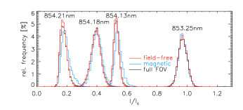
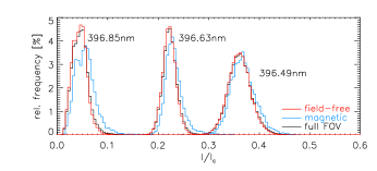
Figure 4: Intensity histograms at selected wavelengths (denoted next to each histogram). Top: Ca ii IR at 854 nm. Bottom: Ca ii H. Black/blue/red lines: full FOV, magnetic locations, and field-free locations.

    

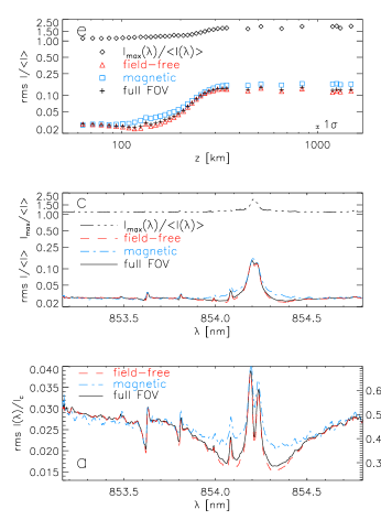
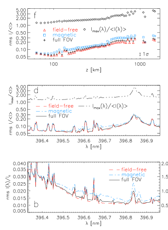
Figure 5: Absolute (bottom row) and relative (middle row) rms variation of the intensity as function of wavelength for Ca ii IR at 854 nm (left) and Ca ii H (right). The solid black lines denote the full FOV, the red dashed and blue dash-dotted lines the field-free and magnetic locations, respectively. Top row: relative fluctuations vs. geometrical height. Black crosses: full FOV. Blue squares: magnetic locations. Red triangles: field-free locations. The ratio of maximum to average intensity is overplotted in the upper two rows with a black dashed triple-dotted line and black diamonds, respectively. The short bars in the lower right corners in panels e and f indicate the average range of scatter for the data points plotted.

The absolute rms values for both lines (panels a and b of Fig. 5) share some common trends. The rms variation reduces from the low-forming (pseudo)continuum wavelength ranges in the far line wing towards the line core, with profound minima for Ca ii IR around 854.1 nm and 854.35 nm, respectively. Near the line cores, the absolute rms values increase again strongly. For the Ca ii IR line at 854.2 nm, the maximum absolute rms value is reached near the line core, for Ca ii H in the line wing. This should be related to the significantly steeper line profile of the Ca ii IR line, where Doppler shifts of the absorption profile will yield large variations of the intensity values taken at a fixed wavelength. The large rms fluctuations in the line wing of Ca ii H are caused by the contrast of the granulation pattern, coupled with the high sensitivity to temperature at the near-UV wavelength. For both lines, the field-free locations show the smallest rms variations at almost all wavelengths. On magnetic locations, the rms value reduces less than for the other two samples in an intermediate range from 853.8 nm (396.45 nm) to the line core. Near the very line core, the Ca ii H line has a clear asymmetry between the wavelengths of the red and blue emission peaks H_2R and H_2V, with larger rms variations for H_2V. The rms values of Ca ii IR just to the red and blue of the line core mimick this asymmetry, even if the average intensity profile of the latter does not show prominent emission peaks.

The relative rms values (panels c and d of Fig. 5) behave quite similar to the absolute rms values, but the minimum of rms fluctuations is much less pronounced for the Ca ii IR line at 854.2 nm and nearly completely vanishes for the magnetic locations (blue line in left middle panel). The relative rms variations of the intensity near the line core are about 20 % (30 %) for Ca ii IR (Ca ii H). The ratio of maximal and average intensity (dash-dotted line in panels c and d of Fig. 5) reaches up to a factor of two for Ca ii IR and about four for Ca ii H, i.e., the intensity can more than double relative to the average value. Because the intensity histograms start to be asymmetric for wavelengths close to the line core (Fig. 4), the rms value presumably slightly underestimates the full amount of the fluctuations, which also do not have the same range towards higher or lower than average intensities.

The upper panels e and f of Fig. 5 show the relative rms fluctuations vs. geometrical height. The conversion from wavelength to geometrical height was done by attributing the optical depth value at the center of the intensity response function to each wavelength, and then using the geometrical height corresponding to that optical depth in a reference atmosphere model (see Appendix C, or also Leenaarts et al. 2010). Each observed spectral range covered several hundred wavelength points, but especially in the line wing several wavelengths are attributed to the same or a very similar geometrical height (cf. the lower panel of Fig. 11). To avoid overcrowding, we plotted only the average value of the rms fluctuations on all unique height points (about 70 values). As estimate of the scatter at one given height, we averaged the range of scatter on all of the data points plotted (short bars in the lower right corners of panels e and f). The scatter at some specific heights can be much larger (cf. the right panel of Fig. 8 later on). In the plots of the relative rms fluctuations vs. geometrical height (top panels of Fig. 5), the fluctuations monotonically increase with height after passing through a minimum between 100 km and 200 km height. They level off to a plateau at about 500 – 700 km height.

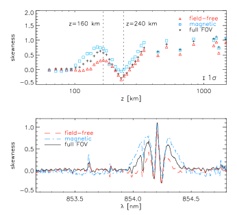
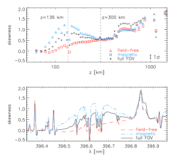
Figure 6: Skewness as function of wavelength (bottom) and vs. geometrical height (top) for Ca ii IR at 854 nm (left) and Ca ii H (right). Same labels and notation as in Fig. 5.

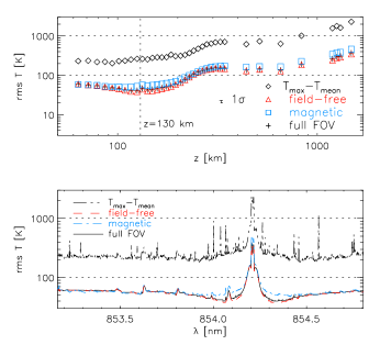
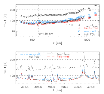
Figure 7: Rms fluctuations of brightness temperature vs. wavelength (bottom row) and geometrical height (top row). Left column: Ca ii IR at 854 nm. Right column: Ca ii H at 396 nm. The difference of maximum and average temperature is overplotted with a black dashed triple-dotted line and black diamonds, respectively. Other labels and notation are as in Fig. 5.

4.4 Skewness of distributions of $I(\lambda)$

The skewness of the intensity distributions is defined as

$${\rm Skewness}=\frac{1}{N}\sum_{j=1}^{N}\left(\frac{x_{j}-\bar{x}}{\sigma}\right)^{3}\;,$$ (1)

where $N$ is the total number of sample points $x_{i}$ and $\sigma$ the standard deviation (Press et al. 1992, Chapter 14).

The individual histograms in Fig. 4 already hinted at a variation of the skewness with wavelength as well as between the three samples. Figure 6 shows the skewness as function of wavelength (lower panels) and vs. geometrical height (upper panels). The differences between the three samples are similar to that in the rms variations, with the magnetic field locations showing largest and the field-free locations the smallest values, but they are much more pronounced here. In a wavelength range intermediate between line wing and core (853.9 – 854.15 nm and 396.45 –396.75 nm), the magnetic locations exhibit a skewness larger by about a factor of two than the field-free locations, with the skewness of the full FOV in the middle between the others. This large difference is maintained up to close to the line core, where the skewness becomes nearly identical again.

The maximal difference of the skewness between magnetic and field-free locations is reached at wavelengths that form at geometrical heights of about 150 km for both spectral lines (top panels of Fig. 6). At a height of about 250 – 300 km, the skewness values equalize again. Both spectral lines contain several line blends that could be the reason for the difference in skewness between the three samples in the FOV, but the same plot as in the upper panels of Fig. 6 using only wavelengths outside of line blends yielded the same behaviour. Doppler shifts of the whole line profile presumably can also be excluded as a reason for the difference in skewness, because for instance for Ca ii H the slope of the line profile is rather small in the wavelength region of the largest difference in skewness. It thus indicates a significant difference of the intensity distributions between the outer wing and the line core on locations with and without magnetic fields.

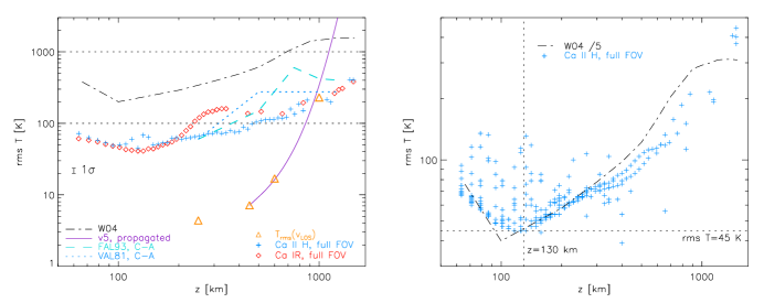
Figure 8: Rms fluctuations of temperature vs. geometrical height in comparison to other measurements (left). Orange triangles: temperature fluctuations corresponding to observed rms LOS velocity (BE09). Purple solid line: propagated LOS velocity of Fe i at 396.6 nm converted to the corresponding temperature equivalent (BE09). Black dash-dotted: rms of the kinetic temperature in the 3D HD simulation of WE04 as read off from their Fig. 9. Blue dotted line: temperature difference of models C and A in VAL81. Turquoise dashed line: the same for FAL93. Red diamonds/blue crosses: temperature fluctuations corresponding to the intensity of Ca ii IR and Ca ii H, respectively. Right: temperature fluctuations corresponding to the intensity of Ca ii H (blue crosses) and rms of the kinetic temperature of WE04 divided by 5 (dash-dotted line).

4.5 Conversion from intensity to temperature fluctuations

The observed (absolute) intensities cannot directly be converted to corresponding gas temperatures without solving the radiative transfer equation, but the relative intensity fluctuations can be approximately converted to brightness temperature fluctuations using the Planck curve. The intensity response functions (Appendix C) provide a mapping from a wavelength $\lambda$ to a corresponding optical depth $\tau(\lambda)$ – taken to be the center of the intensity response function – and hence, to the average temperature $T(\tau(\lambda))$ as given in a reference atmosphere model. If one assumes that the average intensity at one wavelength $I_{\rm mean}(\lambda)$ corresponds to the temperature $T_{0}(\tau)$ predicted by the reference atmosphere model for the respective optical depth $\tau(\lambda)$, the deviation $\Delta I$ from the average intensity value can be attributed to a variation $\Delta T$ of the temperature. The modulus of the temperature variation can be estimated using the Planck curve (Appendix D). We used the Harvard Smithsonian Reference Atmosphere model (HSRA, Gingerich et al. 1971) as temperature reference.

Figure 7 shows the resulting rms fluctuations of brightness temperature as function of wavelength and geometrical height for the Ca ii IR (left column) and the Ca ii H line (right column), respectively. The rms fluctuations of brightness temperature show a minimum of about 45 K at heights of about 130 km and do not exceed 100 K up to a height of about 300 km. They reach values of about 500 K at 1 Mm height. The maximal deviation T_max-T_mean (dotted lines and black diamonds in Fig. 7) from the reference model is about 200 K in the line wing (or lower photosphere), increases nearly monotonically with height in the atmosphere, and exceeds 1000 K at $z\sim 800\,$km. Because of the increasing deviations from LTE with height in the solar atmosphere, the conversion should differ successively more from the kinetic temperature the higher a given wavelength forms in the solar atmosphere.

Figure 8 compares the rms fluctuations of brightness temperature derived from the intensity rms (red diamonds for Ca ii IR and blue crosses for Ca ii H) with other results for the gas temperature rms in the solar atmosphere. As two examples of the variation in semi-empirical static temperature models, we chose the temperature difference between the models C (average internetwork area) and A (chromospheric faint location in quiet Sun) of Vernazza et al. (1981, VAL81, blue dotted line in Fig. 8) and Fontenla et al. (1993, FAL93, turquoise dashed line in Fig. 8), following the approach of Kalkofen (2012). From the first paper of this series (BE09), we took the rms temperature fluctuations corresponding to observed rms line-of-sight (LOS) line-core velocities. The energy content of the rms LOS velocities was converted to the corresponding enhancement of gas temperature by equating the increase of the internal energy and the mechanical energy (orange triangles). In addition to the observed rms velocities, we also overplotted the curve obtained by propagating the LOS velocity of the Fe i line at 396.6 nm to higher layers in the limit of linear perturbation theory and subsequently converting the resulting rms velocities again to the equivalent temperature variation (purple solid line). Finally, the black dash-dotted line shows the rms of the kinetic temperature in a numerical 3D HD simulation done with the CO⁵BOLD code (Freytag et al. 2012) as given in Fig. 9 of Wedemeyer-Böhm et al. (2004, WE04). The latter matches the shape of the temperature rms curve derived from the Ca ii H intensity surprisingly well, but is a factor of about five larger (right panel). In this case, the temperature rms fluctuations of all 326 wavelengths points of the Ca ii H spectra were plotted individually without averaging. The increased scatter below a height of about 200 km is caused by wavelengths in the wing and core of the line blends.

The rms variations from all different approaches share, however, the following properties: a) a local minimum of rms fluctuations at about $z=130$ km, b) a steepening of the curves at about $z=500$ km, and c) rms fluctuations of about 300 – 400 K at about $z=1000$ km. The energy equivalent of the rms LOS velocities below $z=1000$ km falls short by an order of magnitude or more in comparison to the other values. The difference between the “cool” and average semi-empirical models (VAL/FAL C$-$A) matches the rms variation found from the intensity fluctuations around $z=1000$ km.

5 Summary and Discussion

5.1 Summary

The spectral lines of Ca ii H and Ca ii IR at 854.2 nm cover smoothly formation heights from the continuum forming layers of the solar atmosphere in the line wing to the lower chromosphere in the line core. This offers the possibility to obtain information on the solar atmosphere not only from absolute values of observed quantities, but also already from their relative variation throughout the lines. As far as the intensity statistics are concerned, the two lines behave nearly identical, with the following common characteristics: 1. a general increase of the relative rms fluctuations $\sigma_{I}/I_{\rm mean}$ from the line wing to the line core, with minimal rms at wavelengths forming in the low photosphere at about 130 km height. The range of fluctuations is between 3 % to 30 % rms and up to 400 % maximum variation at the line core. 2. Larger rms fluctuations on locations with magnetic fields than on field-free locations. 3. A variable skewness of the intensity distributions caused by extended tails towards high intensities. 4. A pronounced local maximum of the skewness for locations with magnetic fields at intermediate wavelengths of 853.9 – 854.15 nm and 396.45 –396.75 nm. 5. The temperature difference between the original and a modified HSRA model without chromospheric temperature rise ($\equiv$ an atmosphere in radiative equilibrium) is about 1000 K at a height of 1 Mm (Fig. 13, BE09). The rms variations of temperature from either the velocity or the intensity fluctuations do not reproduce such an average temperature enhancement because they suffice only for an enhancement of at maximum about 500 K. We remark that the observations had a spatial resolution of about 1^′′.

5.2 RMS of intensity and temperature fluctuations

After passing through a minimum of the fluctuations at about 130 km height ($\log\tau\approx-1$) caused by the reduction of the granulation contrast (cf.  Puschmann et al. 2003, 2005), the rms fluctuations indicate an increase with height in the solar atmosphere that is expected for upwards propagating acoustic waves with a steepening of the wave amplitude caused by the exponentially decreasing gas pressure. The fluctuations are larger on locations co-spatial to photospheric magnetic fields. To evaluate the significance of the differences in the mean and rms variations between the magnetic and field-free samples (Figs. 4 and 5, and Table B.1), we used a t-Student test and F-test (Press et al. 1992). These tests indicated that the differences are significant by a large margin. The rms fluctuations amount to 61 W/m^-2ster^-1 in a 0.1 nm window around the Ca ii H line core and to 31 W/m^-2ster^-1 for a similar wavelength window around the Ca ii IR line core, where the maximal variations can be much larger than that.

We converted the relative intensity fluctuations to the corresponding brightness temperature variation using the Planck curve, implicitly assuming LTE in the approach. This yielded rms fluctuations of the brightness temperature below 100 K for the photosphere up to $z\sim 300$ km, and up to 500 K in the lower chromosphere at $z\sim 1$ Mm. The trend of brightness temperature fluctuations with height derived from the intensity at different wavelengths in the Ca ii H line matches that in the rms fluctuations of the kinetic temperature in the 3D HD simulations of WE04, but the latter values are larger by a factor of about five. Part of this discrepancy can be attributed to the spatial resolution of about 1^′′ of the data used here. Improving the spatial resolution from 1^′′ to, for instance, the 0$\aas@@fstack{\prime\prime}$32 of the Hinode/SP (Kosugi et al. 2007) increases the rms variations by a factor of about 2 – 3 (Puschmann & Beck 2011, Table 3). For Ca ii IR, data at higher spatial resolution than ours can currently be obtained with IBIS at the Dunn Solar Telescope or CRISP at the Swedish Solar Telescope (Scharmer et al. 2008). The GREGOR Fabry-Perót Interferometer (cf. Puschmann et al. 2011, and references therein) will provide another source of Ca ii IR spectra at 0$\aas@@fstack{\prime\prime}$14 in the near future. The match of our observed temperature rms and the recently published temperature rms in numerical simulations in Freytag et al. (2012, upper right panel of their Fig. 9) would presumably be better than the match with WE04 already without any artificial down-scaling of the fluctuations in the simulations, but their simulations cover only a smaller height range compared to WE04.

5.3 Skewness of intensity distributions

A (large) positive skewness of a probability distribution indicates an extended tail of values above the mean value. The skewness as characteristic quantity, however, has to be taken with care because even a perfectly symmetric Gaussian distribution can yield a non-zero skewness in a limited sample. The standard deviation of the skewness for a normal distribution is given approximately by $\sqrt{15/N}$, where $N$ denotes the number of sample points (Press et al. 1992). In our case, $N\,\approx 10.000$ for the smallest of the samples in the FOV, which yields a standard variation of the skewness of about 0.04. Hence, all measured values of skewness (Fig. 6) above about 0.1 should be significant.

The skewness of the observed intensity distributions is generally positive, close to zero in the line wing/lower heights and up to two near the line core. This implies a more frequent occurrence of excursions towards high intensities, which is expected for acoustic waves forming “hot” shock fronts, not “cold” ones. The positive skewness would also fit to the existence of a limiting energetically lowest state of the atmosphere, e.g., given by an atmosphere in radiative equilibrium or with a stationary chromospheric temperature rise (“basal energy flux”, Schrijver 1995; Schröder et al. 2012), that intermittently is raised to a transient state of higher energy content. The basal flux would prevent the temperature, and hence the intensity from decreasing below some certain critical level, similar to the effect of a thermostat set to prevent freezing. On the upper end of the intensity range, the basal flux would, however, not impose any limitations on the maximum possible intensity value (cf. also Rezaei et al. 2007a). In the presence of a basal energy flux one therefore would not expect to find a negative skewness for chromospheric intensities in the QS because the intensity distribution should have a (rigid) lower limit that cannot be exceeded, but no upper limit (cf., e.g., the intensity distribution at 854.21 nm in the upper panel of Fig. 4). It would be interesting to evaluate the skewness of emergent intensities in numerical simulations for comparison to our observational findings.

The source of the observed skewness values in the intermediate wavelength range (Fig. 6) remains elusive. High-intensity events at heights below 300 km cause a distinct skewness pattern on magnetic regions compared to the field-free area. These events should be different from the shock fronts of steepening acoustic waves found at about 1 Mm that induce the asymmetry of the intensity distributions near the line cores. At a height of 300 km acoustic waves are still in the linear regime without strong damping by, e.g., radiative losses. Section 5.6 below discusses some possible processes that could modify the skewness in the presence of magnetic fields. The remarkably large skewness at the very line core of both lines, i.e., $z\,\approx\,1$ Mm, originates from intensity brightenings caused by hot shock fronts at those heights. Unlike in the line wing, there is no difference of skewness between the magnetic and field-free locations in the line core. Hence, our results indicate rather different origins for the enhanced skewness in the wing and the core of the two lines.

5.4 Assumptions and uncertainties

The discrepancy between the observed and model temperature variations (Fig. 8) depends on the rather long list of (strong) assumptions used in the derivation of the temperature fluctuations from the observed spectra. We try to estimate the error from different steps in the conversion in the following.

Relation between wavelengths and formation heights:

We attributed a specific geometrical height to a given wavelength using the intensity response functions in a static model atmosphere, ignoring both the variable width of the formation height at each wavelength and the dynamical character of the solar chromosphere. To test at least the dependence of the formation height on the selected model atmosphere, we repeated the calculation for the original and the modified HSRA model for the Ca ii H line (bottom panel of Fig. 9). Because the two model atmospheres are identical up to $\log\tau\sim-4$, only wavelengths near the line core change (black crosses in the bottom panel of Fig. 9). Using the original HSRA model slightly reduces the formation height of the line core and raises a bit that of the two emission peaks. The modified HSRA model matches, however, the formation heights derived from the slope of phase differences (see BE08) around $\lambda\sim 396.82$ nm and $396.87$ nm better than the original HRSA model. The measurements of the phase differences are done in a dynamical atmosphere and therefore take spatial and temporal variations of the photospheric and chromospheric structure into account. The uncertainty in the formation height would slightly compress or expand all plots vs. geometrical height, but would not change the general slopes of the curves. The derivation of formation heights from phase differences could be repeated for the Ca ii IR line at 854.2 nm with the data set No. 4.

Effect of Doppler shifts:

The intensity fluctuations attributed to a specific wavelength could also have some intrinsic flaw. Part of the scatter in intensity could come from large-scale macroscopic Doppler shifts that displace the complete absorption profile. For the data used here, this should, however, mainly affect the Ca ii IR line because of its steeper absorption profile near the line core. For the Ca ii H spectra from POLIS with a spectral sampling of 1.92 pm – corresponding to a velocity dispersion of about 1.5 kms^-1 per pixel – and given the mild slope in the line wing of the Ca ii H line, the intensity scatter outside any line core should only reflect true changes of the intensity at a given wavelength and not intensity variations caused by Doppler displacements of the line.

As a test, we created a statistical sample of 50.000 Ca ii H profiles by Doppler shifting an average observed profile with random Gaussian velocities with an rms value of 1 kms^-1. The resulting intensity rms (middle panel of Fig. 9) is close to zero outside of all line blends, but around each line blend the Doppler shifts induce a significant rms intensity fluctuation comparable to the observed values (bottom right panel in Fig. 5). These additional fluctuations caused by Doppler shifts presumably are reflected in, e.g., the increased scatter between 50 and 150 km height in the right panel of Fig. 8, whereas the wavelengths outside the line blends yield the majority of the points that follow a rather smooth curve of lower rms fluctuations. We note that Doppler shifts cannot be the cause of the positive skewness of the intensity distributions, but broaden the intensity histograms because of the similar occurrence rates of blue and red shifts.

Reference model atmosphere and LTE assumption:

The most critical effect in the derivation of the temperature fluctuations is of course the LTE assumption, but also the choice of the reference model and the lack of treatment of the complete line formation in the radiative transfer have an effect on the retrieved temperature fluctuations. The latter is partly compensated because only relative variations are considered, i.e., the variation of the line shape (temperature gradient) compared to the average shape. For the conversion from intensity to temperature fluctuations, we tested the effect of selecting a specific temperature stratification by using the original or the modified HSRA model (top panel of Fig. 9). The solar atmosphere presumably fluctuates roughly between these two cases, with the modified HSRA as lower boundary case. Throughout most of the line wing, the rms stays again unchanged because only the upper layers of the HSRA model were modified. The temperature rms fluctuations in the line core reduce by a factor of up to four when the modified version of the HSRA is used. The reason is that to first order the relative intensity variation is proportional to the relative temperature change times $T^{-1}$ (cf. Eq. 4).

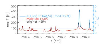
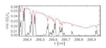
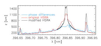
Figure 9: Derivation of error estimates for Ca ii H. Bottom: formation heights in the original (red) and modified HSRA model (black). The blue line gives the formation height from phase differences. Middle: rms fluctuations induced by random Doppler shifts (black). The red line shows an average profile. Top: temperature rms using the original (black) and modified HSRA model (red). Their ratio is given by the blue line with the axis on the right-hand side.

With respect to the LTE assumption, it is unfortunately difficult to estimate in which direction NLTE effects would change the result. On the one hand, NLTE predicts that the same increase in gas temperature will yield a lower increase in intensity than in LTE because the energy is unevenly distributed over the available degree of freedoms, and thus may result in, e.g., ionization imbalances instead of increased radiation. On the other hand, the numerical simulations and experiments by, e.g., Rammacher & Ulmschneider (1992), Carlsson & Stein (1997), or WE04 yield that the basic process related to propagating waves in the solar chromosphere is a compression of material to hot shock fronts, whose increased temperature leads to enhanced emission. How much the conditions in the relevant small-scale shock fronts and their immediate surroundings then deviate from LTE is not clear at once because there are effects present that can either decrease or increase the source function relative to the Planck function (Rammacher & Ulmschneider 1992; Carlsson & Stein 1997). It is, however, expected that the LTE approach underestimates the true temperature fluctuations, but by which amount cannot be derived straightforwardly.

The fact that the observed and theoretical curves of temperature fluctuations in the right panel of Fig. 8 can be roughly matched with a constant coefficient implies that despite all the simplifying assumptions both the attributed geometrical formation heights and the temperature rms cannot be completely off. Neglecting NLTE effects should have a significant impact above a height of about 400 km (e.g., Rammacher & Ulmschneider 1992), but should presumably introduce an ever increasing deviation with height that is not seen as such. We plan to eventually extend the analysis of the data to a proper NLTE investigation using the inversion code of Socas-Navarro et al. (2000) in the future, but propose to provide the data used in the present study to anybody interested in improving the diagnostics of the analysis by including NLTE effects.

Mask of magnetic locations:

The increased skewness at intermediate wavelengths/heights (150 – 300 km) implies more high-intensity events at these layers in the presence of photospheric magnetic fields. We note that for the derivation of the polarisation masks defining field-free and magnetic locations we have only used the circular polarisation signal, because the Stokes $Q$ and $U$ signals are usually one order of magnitude smaller in QS. The magnetic locations thus neither correspond to horizontal nor vertical magnetic fields, but any orientation between these extremes that still produces a measurable circular polarisation signal above the detection limit of the observations (down to a few $10^{-4}$ of $I_{c}$ for observation No. 3). This covers then network regions, isolated “collapsed” structures (i.e., evacuated and concentrated magnetic flux, cf.  Stenflo 2010), their immediate surroundings, and also all types of transient polarisation signals above the threshold used. We therefore cannot directly identify which kind of solar magnetic structure is related to increased intensity in the line wing in the statistic sample, but a study of individual events should allow one to pinpoint the corresponding magnetic features.

5.5 Semi-empirical vs. dynamic chromospheric models

For the discussion on the validity of semi-empirical (e.g., HSRA, VAL81, FAL93, Fontenla et al. 2006; Avrett & Loeser 2008) vs. dynamic chromospheric temperature models (e.g., Carlsson & Stein 1997; Gudiksen et al. 2011, WE04) our observations add that both Ca ii lines used here show large rms intensity fluctuations (up to 30 %) and a very dynamic behaviour, as also found by Cram & Dame (1983) for Ca ii H, and Cauzzi et al. (2008) or Vecchio et al. (2009) for the Ca ii IR line at 854.2 nm. This favors dynamical models of the chromosphere more than the semi-empirical approaches that match average spectra without or with low spatial and temporal resolution. Avrett (2007) states that temperature variations of 400 K cause an intensity variation in excess of “ the observed intensity variations at chromospheric wavelengths”. A similar line of argumentation is used in Kalkofen (2012), going back to a quote from Carlsson et al. (1997) that “all chromospheric lines show emission above the continuum everywhere, all the time”. There is, however, one big caveat in these claims: the Ca ii lines were not considered in the latter works, only the lines and continua observed with SUMER/SOHO and/or atlas spectra. Indeed, the observations of reversal-free Ca profiles challenge a chromosphere which is permanently hot everywhere (Rezaei et al. 2008).

The discrepancy between the dynamical and stationary view of the solar chromosphere here does neither depend on the way of evaluating the data nor the assumption of LTE or NLTE in the analysis. It is a clear fact that the observed spectra of Ca ii lines with their complete change from (strong) emission to reversal-free absorption profiles contradict the SUMER observations with permanent and ubiquitous emission with only a minor variation. As already suggested in BE08, this contradictory behaviour of all these so-called “chromospheric” spectral lines could be reconciled by a single cause, namely, if the SUMER UV and the Ca ii lines do not form at the same height in the solar atmosphere. Carlsson & Stein (1997) found in their dynamical NLTE simulations a formation height of Ca ii H of about 1 Mm, which is about 1 Mm lower than in static 1D models (e.g., Fig. 1 in VAL81). The variation in the formation height of the Ca ii H line core is significantly larger than that of photospheric lines. While the former suffers from a spatially and temporally (strongly) corrugated landscape in the source function, the latter benefit from a rather smooth variation of the formation height. Hence, it seems highly desirable to check the formation heights of the UV lines and continua observed with SUMER in dynamical atmosphere models or numerical simulations. It is possible that opposite to Ca ii H their formation heights would have to be significantly raised in a dynamical atmosphere, putting them above an existing magnetic canopy that dampens all oscillations.

Moll et al. (2012) recently found that the presence of magnetic fields strongly affects the flow field in the upper photosphere and consequently the photospheric and chromospheric heating. As a result, it is important to repeat dynamic models such as those of WE04 and Carlsson & Stein (1997) with an inclusion of magnetic fields. Basically all chromospheric simulations up to today share simplifications regarding the topology or presence of small-scale magnetic fields, scattering, time-dependent hydrogen ionization, as well as the NLTE radiative transfer (Carlsson & Leenaarts 2012).

5.6 Energy sources for the chromospheric radiative losses

An atmosphere in radiative equilibrium has no temperature rise. Therefore, an enhanced chromospheric temperature requires some energy transfer to the upper layers of the solar atmosphere, resulting in emission of the spectral line cores. This, however, is distinctly different from the enhanced emission one finds, e.g., in network bright points. There, a partial evacuation of the atmosphere and the related shift of the optical depth scale cause the excess emission. In other words, magnetic bright points and faculae are (quasi-stationary) bright because of the Wilson depression (Keller et al. 2004; Steiner 2005; Hirzberger & Wiehr 2005). The enhanced skewness on magnetic locations at intermediate wavelengths therefore could result from the spatial variation of the optical depth scale in the presence of magnetic fields of variable total magnetic flux. The high-intensity events in the line wing then should show a close spatial or temporal correlation to the total magnetic flux if they are solely caused by optical depth effects.

Opposite to that, chromospheric transient brightenings such as bright grains (e.g., Rutten & Uitenbroek 1991) are believed to result from a temporary energy deposit. The intensity enhancements in the line wing could be similar to bright grains, but the source of the energy deposit in that case is unclear. The primary suspect would be the abundant waves in the solar atmosphere. The propagation and refraction of acoustic and magneto-acoustic waves in and around magnetic flux concentrations can generate strong upflows or downflows (e.g., Kato et al. 2011). Beside that, the swaying motions of magnetic elements in the convectively unstable photosphere (Steiner et al. 1998; Rutten et al. 2008) result in shock waves propagating inside and outside magnetic flux concentrations (Vigeesh et al. 2011). Such spontaneous excitations of shock fronts is another alternative mechanism for an energy deposit in the lower solar atmosphere.

Several studies show that a conversion between hydrodynamic waves and different types of magneto-acoustic wave modes is possible near the equipartition layer of similar sound and Alfvén speed (cf. Cally 2007; Haberreiter & Finsterle 2010; Nutto et al. 2010a, b). The latter authors investigated wave propagation in numerical magneto-hydrodynamical (MHD) 2D simulations, in which the equipartition layer can be seen to be located near a height of 300 km close to a magnetic field concentration (Nutto et al. 2010b, their Fig. 1). Nevertheless, pure mode conversion does not deposit energy into the atmosphere and therefore should not increase the occurrence rate of high-intensity events. Contrary to that, Davila & Chitre (1991) discuss resonance absorption of acoustic waves as a possible candidate for an energy deposit in the presence of a (horizontal) magnetic canopy. Numerical simulations should be capable to address this problem, e.g., by extending the studies of Leenaarts & Wedemeyer-Böhm (2005) and Leenaarts et al. (2009) from filter imaging to an investigation of the full line spectrum of the Ca ii lines (including the line blends) and by including magnetic fields into the simulations. This should allow one to determine whether the characteristic differences between magnetic and field-free locations in terms of the skewness found in the observations show up as well in spectra synthesized from MHD simulations.

Magnetic reconnection or flux cancellation (e.g., Bellot Rubio & Beck 2005; Beck et al. 2005a) are alternative options for releasing thermal energy in only certain layers of the atmosphere. Such events are more likely to occur in the moat of sunspots or emerging flux regions where an extensive rearrangement of the magnetic field lines happens (e.g., Pariat et al. 2004). These energetic events occur below and above the temperature minimum (e.g., Tziotziou et al. 2005; Yurchyshyn et al. 2010; Watanabe et al. 2011). Even if such high-energy events are not common in QS, granular-scale flux cancellation happens more frequently (Rezaei et al. 2007b; Kubo et al. 2010). The necessary amount of “new” magnetic flux for a repeated occurrence of such events can be provided by small-scale flux emergence in the QS (e.g., Gömöry et al. 2010, and references therein) that can effect an energy transport from below the photosphere to the chromosphere. Part of the newly-emerged emergent flux can reach the lower or upper chromosphere (Martínez González & Bellot Rubio 2009). The two time-series used in the present study (cf. Fig. 1 and BE08) show several cases of transient polarisation signals that could indicate flux emergence events. This allows one a case study of individual brightening events in the line wing on a possible relation to co-spatial or close-by flux emergence, but is beyond the scope of the present study.

6 Conclusions

The intensity distributions of the chromospheric lines of Ca ii H and the Ca ii IR line at 854.2 nm show a minimum of rms fluctuations for wavelengths forming in the low photosphere caused by the inversion of the granulation pattern. Wavelengths forming above the height of minimal rms show a nearly monotonic increase of rms fluctuations towards the line core that indicates propagating acoustic waves with increasing oscillation amplitudes. A conversion of these intensity fluctuations to corresponding brightness temperature variations yields rms values of about 100 K in the lower photosphere and a few hundred K in the chromosphere, favoring dynamical models of the solar chromosphere. The fluctuations fall still short of those in numerical simulations and would not suffice to lift an atmosphere in radiative equilibrium to the temperature of, e.g., the HSRA model. The positive skewness for most wavelengths indicates a higher occurrence frequency of high-intensity events, presumably the hot shock fronts formed by the steepening acoustic waves. A prominent difference in skewness between magnetic and field-free locations for wavelengths forming in the mid photosphere indicates the existence of a mechanism that operates only in the presence of magnetic fields and enhances the intensity in the line wing. Single-case studies of such events will allow one to identify the exact process and its relation to the structure of the magnetic field.

Appendix A Average profiles

For completeness, Fig. 10 shows the average profiles of the remaining observations used in this study. The average and minimal intensity profiles differ only slightly for both the Ca ii IR line at 854.2 nm and Ca ii H. The maximum observed intensity of Ca ii H varies significantly from observation to observation opposite to the minimum intensity, implying that extreme excursions towards higher intensity happen more frequently than those towards lower intensity.

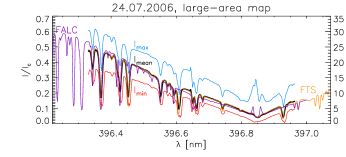
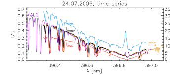
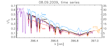
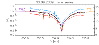
Figure 10: Average Ca ii H profiles of observations No. 1 (top), 2 (3^rd row), and 4 (2^nd row). Bottom: average Ca ii IR profile of observation No. 4. Same layout as Fig. 2.

Appendix B Full statistics at selected wavelengths

Table 2 lists the complete statistics at three (four) wavelengths in the Ca ii H (Ca ii IR) line. The skewness of the magnetic locations is up to three to five times larger than that of the field-free locations for the intermediate wavelengths (396.632 nm and 854.131 nm).

Table 2: Intensity statistics at selected wavelengths. All values but the dimensionless skewness are relative to the continuum intensity $I_{c}$.

$\lambda$ [nm]	region	$I_{\rm min}$	$I_{\rm av}$	$I_{\rm max}$	$\sigma$	skewness
396.486	full FOV	0.274	0.366	0.464	0.022	0.044
	field-free	0.274	0.365	0.450	0.022	-0.063
	magnetic	0.288	0.373	0.464	0.024	0.282
396.632	full FOV	0.183	0.228	0.332	0.014	0.792
	field-free	0.183	0.227	0.295	0.012	0.258
	magnetic	0.190	0.236	0.332	0.018	1.221
396.847	full FOV	0.026	0.053	0.204	0.013	1.854
	field-free	0.026	0.052	0.194	0.011	1.602
	magnetic	0.031	0.063	0.188	0.018	1.563
853.245	full FOV	0.864	0.981	1.087	0.029	0.002
	field-free	0.867	0.980	1.085	0.029	-0.014
	magnetic	0.880	0.980	1.080	0.028	-0.051
854.131	full FOV	0.473	0.540	0.653	0.019	0.605
	field-free	0.473	0.539	0.616	0.017	0.289
	magnetic	0.482	0.553	0.653	0.024	0.743
854.180	full FOV	0.256	0.403	0.538	0.033	-0.182
	field-free	0.264	0.401	0.531	0.032	-0.225
	magnetic	0.268	0.410	0.535	0.034	-0.036
854.213	full FOV	0.128	0.189	0.338	0.023	0.989
	field-free	0.128	0.188	0.324	0.021	0.744
	magnetic	0.136	0.203	0.337	0.030	0.931

Appendix C Intensity response function for the Ca ii IR line at 854.2 nm

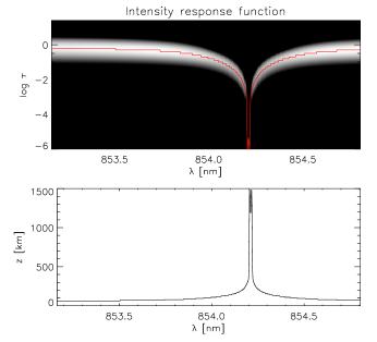
Figure 11: Conversion from wavelength to geometrical height for the Ca ii IR at line 854.2 nm. Top: intensity response function. The red line denotes the centre of the response function at each wavelength. Bottom: geometrical height corresponding to the centre of the response function.

To determine the formation height of a given wavelength in the Ca ii lines, we synthesized the spectral lines with the SIR code (Ruiz Cobo & del Toro Iniesta 1992) in LTE using a modified version of the HSRA model (Gingerich et al. 1971) without chromospheric temperature rise (cf. BE09). Using the original HSRA model yielded comparable results (see Fig. 9 for the case of Ca ii H). The two atmosphere models are fully identical up to $\log\tau=-4$. We added a temperature perturbation of 1 K to each of the 75 points in optical depth one after the other and synthesized the corresponding spectra. The difference to the unperturbed profile $\Delta I(\lambda,\tau)=I(\lambda,T+\Delta T(\tau))-I(\lambda,T)$ yields the intensity response function with wavelength for perturbations at a given optical depth (upper panel of Fig. 11). For each $\lambda$, we fitted a Gaussian to $\Delta I(\lambda,\tau)$, where the centre of the Gaussian yields the optical depth attributed to that wavelength, $\tau(\lambda)$. With the tabulated values of $\tau$ and $z$ in the original HSRA model, one can then obtain the corresponding geometrical height, $z(\lambda)$ (lower panel of Fig. 11). The respective curve for Ca ii H was derived fully analogously (see, e.g., BE09). The attributed formation heights from the intensity response function match well those derived from phase differences (BE08, BE09, their Fig. 1).

Appendix D Conversion between intensity and brightness temperature fluctuations using the Planck curve

Figure 12: Calculation of brightness temperature variation corresponding to intensity fluctuations of $\pm\sigma_{I}/I_{\rm mean}$. Top: for $\lambda=854.213$ nm in the core of the Ca ii IR line. Bottom: for $\lambda=396.847$ nm in the core of the Ca ii H line.

For the conversion from relative intensity fluctuations to brightness temperature fluctuations, one needs first to attribute a characteristic temperature to the average intensity at each wavelength. To that extent, we used the results of the previous section. The centre of the intensity response function at each wavelength $\lambda$ yields the optical depth $\tau(\lambda)$ corresponding to that wavelength (e.g., third column of Table 3). The reference atmosphere model then provides the temperature $T_{0}(\tau)$ at that optical depth, where we assume that the average intensity $I_{\rm mean}(\lambda)$ at the wavelength is directly related to the average temperature $T_{0}(\tau(\lambda))$ . In the LTE assumption, this relation between intensity and temperature is given by:

$$I_{\rm mean}(\lambda,T_{0})=\frac{2\pi hc^{2}}{\lambda^{5}}\cdot\frac{1}{\exp^{\left(\frac{hc}{\lambda kT_{0}}\right)}-1}\equiv I_{0}(\lambda,T_{0})\,.$$ (2)

For a given intensity variation, e.g., by the rms fluctuation $\sigma_{I}$, one obtains that

$$\frac{I_{\rm mean}\pm\sigma_{I}}{I_{\rm mean}}(\lambda)=\frac{I(\lambda,T_{0}\pm\Delta T)}{I_{0}(\lambda,T_{0})}\;.$$ (3)

For $\frac{hc}{\lambda kT_{0}}\gg 1$, one obtains

$$\frac{\Delta I}{I_{0}}\propto\frac{\Delta T}{T_{0}^{2}}\,=\frac{\Delta T}{T_{0}}\cdot\frac{1}{T_{0}}.$$ (4)

Table 3: Parameters and temperature fluctuations at selected wavelengths in Ca ii H.

$\lambda$	$\frac{\sigma_{I}}{I_{\rm mean}}(\lambda)$	log $\tau(\lambda)$	$z(\tau)$	$T_{0}(\tau)$	$T_{-}$	$T_{+}$	$\sigma_{T}$
nm			km	K	K	K	K
396.338	0.066	-0.2	63	6035	5966	6100	67
396.416	0.063	-0.3	71	5890	5830	5948	59
396.492	0.061	-0.4	79	5765	5708	5820	56
396.494	0.061	-0.5	86	5650	5596	5702	53
396.638	0.061	-1.0	125	5160	5118	5200	41
396.650	0.105	-1.1	133	5080	5006	5148	71
396.693	0.074	-1.3	149	4950	4904	4994	45
396.704	0.076	-1.4	158	4895	4848	4940	46
396.773	0.105	-2.1	229	4630	4568	4688	60
396.778	0.109	-2.2	241	4600	4536	4658	61
396.784	0.113	-2.3	253	4575	4510	4636	63
396.786	0.114	-2.4	266	4550	4484	4610	63
396.798	0.124	-2.6	294	4490	4420	4554	67
396.802	0.128	-2.7	309	4460	4388	4526	69
396.804	0.131	-2.8	327	4430	4358	4496	69
396.808	0.135	-2.9	344	4405	4330	4472	71
396.810	0.137	-3.0	362	4380	4306	4448	71
396.812	0.141	-3.1	380	4355	4280	4424	72
396.816	0.150	-3.2	399	4330	4250	4402	76
396.817	0.156	-3.3	420	4305	4224	4378	77
396.819	0.162	-3.4	441	4280	4196	4354	79
396.821	0.170	-3.5	463	4250	4164	4326	81
396.823	0.179	-3.6	489	4225	4136	4304	84
396.825	0.192	-3.7	515	4205	4112	4286	87
396.827	0.206	-3.8	540	4190	4090	4276	93
396.829	0.221	-4.0	595	4170	4064	4260	98
396.831	0.239	-4.1	624	4200	4084	4298	107
396.833	0.256	-4.2	655	4280	4150	4390	120
396.835	0.273	-4.4	721	4530	4372	4660	144
396.837	0.287	-4.6	791	4790	4604	4944	170
396.839	0.294	-4.8	873	5040	4830	5214	192
396.841	0.295	-6.0	1482	7360	6924	7730	403

Because of the non-linearity of Eq. (3), $\Delta T$ is different for adding and subtracting the rms fluctuation from $I_{\rm mean}$. We therefore used the average value of $\Delta T$ for the two signs as the temperature variation that corresponds to the rms intensity fluctuation. To obtain the brightness temperature difference corresponding to the increase/decrease of $I$ by one standard deviation $\sigma_{I}$, the variation of the emergent intensity around the average value $T_{0}$ is calculated with Eq. (2). The relative change of $I/I_{0}(\lambda,T_{0})$ is displayed in Fig. 12 for two wavelengths in the line core of Ca ii H (bottom panel of Fig. 12) and Ca ii IR (top panel of Fig. 12). The temperatures corresponding to 1$\pm\sigma_{I}/I_{\rm mean}(\lambda)$ are then read off from the intersections with the curve of relative intensity variation. Using the modified HSRA model reduces the temperature rms (Fig. 9) because of the dependence on $T^{-1}$ in Eq. (4). We used the original HSRA as temperature reference because the majority of the solar atmosphere should presumably be closer to the original than the modified HSRA model. Table 3 lists the relevant parameters and resulting temperature values for several wavelengths in the Ca ii H line, sorted to have monotonically increasing wavelength and formation heights. We point out that the values of $T_{0}$ and $z$ were taken from the original HSRA model and were not derived from the observed spectra themselves.