Deep exclusive $\pi^{+}$ electroproduction off the proton at CLAS

Abstract

The exclusive electroproduction of $\pi^{+}$ above the resonance region was studied using the $\rm{CEBAF}$ Large Acceptance Spectrometer ($\rm{CLAS}$) at Jefferson Laboratory by scattering a 6 GeV continuous electron beam off a hydrogen target. The large acceptance and good resolution of $\rm{CLAS}$, together with the high luminosity, allowed us to measure the cross section for the $\gamma^{*}p\to n\pi^{+}$ process in 140 ($Q^{2}$, $x_{B}$, $t$) bins: $0.16<x_{B}<0.58$, $1.6$ GeV${}^{2}<$ $Q^{2}$ $<4.5$ GeV² and $0.1$ GeV${}^{2}<$ $-t$ $<5.3$ GeV². For most bins, the statistical accuracy is on the order of a few percent. Differential cross sections are compared to four theoretical models, based either on hadronic or on partonic degrees of freedom. The four models can describe the gross features of the data reasonably well, but differ strongly in their ingredients. In particular, the model based on Generalized Parton Distributions (GPDs) contain the interesting potential to experimentally access transversity GPDs.

1 Introduction

One of the major challenges in contemporary nuclear physics is the study of the transition between hadronic and partonic pictures of the strong interaction. At asymptotically short distances, the strong force is actually weak and the appropriate degrees of freedom are the quarks and gluons (partons) whose interaction can be quantified very precisely by perturbative Quantum Chromodynamics (pQCD). However, at larger distances on the order of one Fermi, effective theories that take hadrons as elementary particles whose interactions are described by the exchange of mesons appear more applicable. The connection between these two domains is not well understood. In order to make progress, a systematic study of a series of hadronic reactions probing these intermediate distance scales is necessary. The exclusive electroproduction of a meson (or of a photon) from a nucleon, $\gamma^{*}N\to N^{\prime}M$, is particularly interesting. Indeed, it offers two ways to vary the scale of the interaction and therefore to study this transition regime. One can vary the virtuality of the incoming photon $Q^{2}=-(p_{e}-p_{e}^{\prime})^{2}$, which effectively represents the transverse size of the probe, or the momentum transfer to the nucleon $t=(p_{N}-p_{N}^{\prime})^{2}$, which effectively represents the transverse size of the target. Here, $p_{e}$ and $p_{e}^{\prime}$ are the initial and scattered electron four-momenta and $p_{N}$ and $p_{N}^{\prime}$ are the initial and final nucleon four-momenta, respectively. Figure 1 sketches the transition regions that have been experimentally explored until now (lightly shaded areas) as a function of these two variables, $Q^{2}$ and $|t|$. In this figure, we keep, quite arbitrarily, only the experiments for which $|t|>$ 3 GeV² in photoproduction ($\rm{SLAC}$ RAnderson00 and $\rm{JLab}$ WChen ) and $Q^{2}>$ 1.5 GeV² in electroproduction (Cornell bebek76 ; bebek78 , $\rm{JLab}$ Horn09 ; HPBlok ; XQian and $\rm{HERMES}$ Hermes ). These are the domains for which, we believe, there are chances to observe first signs that partonic degrees of freedom play a role in the reactions. The darkly shaded area in Fig. 1 represents the phase space covered by the present work. It is divided into 140 ($Q^{2}$, $x_{B}$ or $W$, $t$) bins, to be compared to only a few ($Q^{2}$, $x_{B}$ or $W$, $t$) bins in the lightly shaded areas for the previous electroproduction experiments.

We also display in Fig. 1 three Feynman-type diagrams illustrating the mechanisms believed to be at stake for the $\gamma^{*}N\to N^{\prime}M$ process: at asymptotically large-$Q^{2}$, asymptotically large-$|t|$ (both in terms of partonic degrees of freedom) and at low-$Q^{2}$ and low-$|t|$ (in terms of hadronic degrees of freedom).

At asymptotically large $Q^{2}$ and small $|t|$ (along the vertical axis in Fig. 1), the exclusive electroproduction of a meson should be dominated by the so-called “handbag diagram” muller ; ji ; rady ; JCCollins . The initial virtual photon hits a quark in the nucleon and this same quark, after a single gluon exchange, ends up in the final meson. A QCD factorization theorem JCCollins states that the complex quark and gluon non-perturbative structure of the nucleon is described by the Generalized Parton Distributions (GPDs). For the $\pi^{+}$ channel at leading twist in QCD, i.e. at asymptotically large $Q^{2}$, the longitudinal part of the cross section $\sigma_{L}$ is predicted to be dominant over the transverse part $\sigma_{T}$. Precisely, ${d\sigma_{L}}/{dt}$ should scale as ${1}/{Q^{6}}$ at fixed $x_{B}$ and $|t|$, while ${d\sigma_{T}}/{dt}$ should scale as ${1}/{Q^{8}}$. It is predicted that $\sigma_{L}$ is sensitive to the helicity-dependent GPDs $\tilde{E}$ and $\tilde{H}$ JCCollins while, if higher-twist effects are taken into account and factorization is assumed, $\sigma_{T}$ is sensitive to the transversity GPDs, $H_{T}$ and $\bar{E}_{T}=2\tilde{H}_{T}+E_{T}$ GK09 .

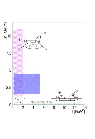
Figure 1: (color online). Schematic representation of the $\gamma^{*}N\to N^{\prime}\pi$ process (above the resonance region) in different regions of the ($Q^{2}$, $t$) plane. The Feynman diagrams describe the reaction in terms of meson exchanges at low $Q^{2}$ and $|t|$, in terms of GPDs at large $Q^{2}$ and small $|t|$, and in terms of hadron distribution amplitudes (DA) at large $|t|$. The lightly shaded areas (magenta and green online) represent approximately the experimentally explored regions up to now. The darkly shaded area (blue online) represents the phase space covered by this work.

At large values of $|t|$, in photoproduction (i.e. along the horizontal axis in Fig. 1) but also presumably in electroproduction, the $\gamma^{(*)}N\to N^{\prime}M$ process should be dominated by the coupling of the (virtual) photon to one of the valence quarks of the nucleon (or of the produced meson), with minimal interactions among the valence quarks. In this regime, a QCD factorization theorem states that the complex structure of the hadrons is described by distribution amplitudes (DA) which at small distances (large $|t|$) can be reduced to the lowest Fock states, i.e. 3 quarks for the nucleon and $q$-$\bar{q}$ for the meson lepage . At sufficiently high energy, constituent counting rules (CCR) SBrodsky00 predict an $s^{-7}$ scaling of the differential cross section ${d\sigma}/{dt}$ at fixed center-of-mass pion angles, provided $|s|$, $|t|$, and $|u|$ are all large. Here $s=W^{2}$ is the squared invariant mass of the $\gamma^{*}$-$p$ system and $u=(p_{\gamma}^{*}-p_{N}^{\prime})^{2}$ is given in terms of the four-vectors $p_{\gamma}^{*}=p_{e}-p_{e}^{\prime}$ and $p_{N}^{\prime}$ for the final-state nucleon. The large $|t|$ and $|u|$ region corresponds typically to a center-of-mass pion angle $\theta_{\rm{cm}}\approx 90^{\circ}$. In this domain, the CCR predict ${d\sigma}/{dt}=f(\theta_{\rm{cm}})s^{2-n}~{}$ for the energy dependence of the cross section, where $f(\theta_{\rm{cm}})$ depends on details of the dynamics of the process and $n$ is the total number of point-like particles and gauge fields in the initial and final states. For example, our reaction $\gamma^{*}p\to n\pi^{+}$ should have $n=9$, since there is one initial photon, three quarks in the initial and the final nucleons, and two in the final pion.

Many questions are open, in particular at which $Q^{2}$ and $s$ do such scaling laws start to appear. Even if these respective scaling regimes are not reached at the present experimentally accessible $Q^{2}$ and $s$ values, can one nevertheless extract GPDs or DAs, provided that some corrections to the QCD leading-twist mechanisms are applied? Only experimental data can help answer such questions.

2 Insights from previous experiments with respect to partonic approaches

The two most recent series of experiments that have measured exclusive $\pi^{+}$ electroproduction off the proton, in the large-$Q^{2}$, low-$|t|$ regime where the GPD formalism is potentially applicable, have been conducted in $\rm{Hall~{}C}$ at Jefferson Lab ($\rm{JLab}$) Horn09 ; HPBlok ; XQian and at $\rm{HERMES}$ Hermes .

The $\rm{Hall~{}C}$ experiments, with 2 to 6 GeV electron beam energies, separated the $\sigma_{L}$ and $\sigma_{T}$ cross sections of the $\gamma^{*}p\to n\pi^{+}$ process using the Rosenbluth technique for $0.17<x_{B}<0.48$ and $Q^{2}$ up to $3.91$ GeV². The term $\sigma_{L}$ dominated the cross section for $|t|<$ 0.2 GeV², while $\sigma_{T}$ was dominant for larger $|t|$ values. These data were compared to two GPD-based calculations, hereafter referred to as VGG VGG00 and GK GK09 ; GK11 from the initials of the models’ authors. The comparison of the data with the VGG model can be found in the Hall C publications Horn09 ; HPBlok while the comparison with the GK model can be found in the GK publications GK09 ; GK11 . For $\sigma_{L}$, which should be the QCD leading-twist contribution, these GPD calculations were found to be in general agreement with the magnitude and the $Q^{2}$- and $t$- dependencies of the experimental data. In these two calculations the main contribution to $\sigma_{L}$ stems from the $\tilde{E}$ GPD, which is modeled either entirely as pion-exchange in the $t$-channel VGG00 or is at least dominated by it GK09 ; GK11 (see Refs. manki ; franki for the connection between the $t$-channel pion-exchange and the $\tilde{E}$ GPD). This term is also called the “pion pole”, and the difference between the two calculations lies in the particular choice made for the $t$-channel pion propagator (Reggeized or not) and the introduction of a hadronic form factor or not at the $\pi NN$ vertex. In both calculations, $\sigma_{L}$ contains higher-twist effects because the pure leading-twist component of the pion pole largely underestimates the data. Only the GK model, which explicitly takes into account higher-twist quark transverse momentum, is able to calculate $\sigma_{T}$. Agreement between data and calculation is found only if the $H_{T}$ transversity GPD is introduced, which makes up most of $\sigma_{T}$.

The $\rm{HERMES}$ experiment used 27.6 GeV electron and positron beams to measure the $\gamma^{*}p\to n\pi^{+}$ cross section at four ($x_{B}$, $Q^{2}$) values, with $x_{B}$ ranging from 0.08 to 0.35 and $Q^{2}$ from 1.5 to 5 GeV². Since all data were taken at a single beam energy, no longitudinal/transverse separation could be carried out. The differential cross section ${d\sigma}/{dt}$ was compared to the same two GPD models mentioned above. The GK model, which calculates both the longitudinal and transverse parts of the cross section, displays the same feature as for the lower energy $\rm{JLab}$ data, i.e. a dominance of $\sigma_{L}$ up to $-t\approx$ 0.2 GeV², after which $\sigma_{T}$ takes over. The sum of the transverse and longitudinal parts of the cross section calculated by the GK model is in very good agreement with the data over most of the $\-t$ range measured at $\rm{HERMES}$ GK09 ; GK11 . The VGG model, which calculates only the longitudinal part of the cross section, is in agreement with the data only for low $t$ values Hermes . Again, in both calculations, $\sigma_{L}$ is dominated by the $\tilde{E}$ GPD, modeled essentially by the pion pole term, and $\sigma_{T}$, in the GK model, is due to the transversity GPDs. The $\rm{HERMES}$ experiment also measured the transverse target spin asymmetry $A_{UT}$ for the $\gamma^{*}p\to n\pi^{+}$ process, which indicate GK09 ; GK11 that the transversity GPDs $H_{T}$ or $\bar{E}_{T}$ indeed play an important role in the process, confirming the approach of the GK group.

The comparison between the $\rm{JLab}$ $\rm{Hall~{}C}$ and HERMES experiments and the two GPD-based calculations yields very encouraging signs that, although higher-twist contributions definitely play a major role, these data can be interpreted in terms of GPDs, in particular transversity GPDs. More precise and extensive data would be highly useful to confirm these findings. Firstly, the present CLAS experiment extends somewhat the ($x_{B}$, $Q^{2}$) phase space previously covered by the $\rm{JLab}$ $\rm{Hall~{}C}$ experiments and secondly, it covers 20 ($x_{B}$, $Q^{2}$) bins (with statistical errors of a few percent on average) which doubles the number of bins of the $\rm{JLab}$ $\rm{Hall~{}C}$ experiments (and triples the $\rm{HERMES}$ number of bins). These new data are important to test the present GPD-based model calculations and, if successful, bring more stringent constraints on the current GPD parametrizations.

The large-$|t|$ (large-$|u|$) domain, where the DA formalism is asymptotically applicable for $\gamma^{(*)}p\to n\pi^{+}$, has so far been explored only in high-energy photoproduction at $\rm{SLAC}$ RAnderson00 and intermediate-energy photoproduction at $\rm{JLab}$ LYZhu . While the $\rm{SLAC}$ data tend to follow the $s^{-7}$ scaling asymptotic prediction, for a $90^{\circ}$ center-of-mass angle, the more recent $\rm{JLab}$ data, which are compatible with the $\rm{SLAC}$ data but are more precise, actually reveal some large oscillations around this $s^{-7}$ behavior.

In recent years a similar trend, i.e. “global” scaling behavior, has been observed in deuteron photo-disintegration experiments JNapolitano00 ; CBochna00 ; ESchulte00 ; PRossi00 , and also in hyperon photoproduction Schumacher:2010qx . It would be interesting to see this in exclusive pion electroproduction and if so, whether the oscillations disappear as $Q^{2}$ increases. The measurement presented in this article is the first one to explore this large-$|t|$, large-$|u|$ domain ($\theta_{\rm{cm}}\approx 90^{\circ}$) for $\sqrt{s}>$ 2 GeV in $\pi^{+}$ exclusive electroproduction off the proton. The present CLAS electroproduction experiment covers a $t$-range up to $\approx$ 5 GeV² while the largest $|t|$-values measured by Hall C are $\approx$ 0.9 GeV² and by HERMES $\approx$ 2 GeV².

3 The Experiment

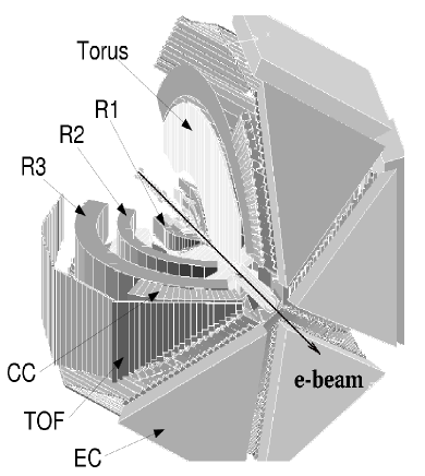
Figure 2: Three-dimensional view of the $\rm{CLAS}$ detector.

The measurement was carried out with the CEBAF Large Acceptance Spectrometer ($\rm{CLAS}$) CLAS . A schematic view of $\rm{CLAS}$ is shown in Fig. 2. $\rm{CLAS}$ has a toroidal magnetic field generated by six flat superconducting coils (main torus), arranged symmetrically around the azimuth. Six identical sectors are independently instrumented with 34 layers of drift cells for particle tracking ($\rm{R1}$, $\rm{R2}$, $\rm{R3}$), plastic scintillation counters for time-of-flight ($\rm{TOF}$) measurements, gas threshold Cherenkov counters ($\rm{CC}$) for electron and pion separation, and electromagnetic calorimeters ($\rm{EC}$) for photon and neutron detection. To aid in electron/pion separation, the $\rm{EC}$ is segmented into an inner part closer to the target and an outer part further away from the target. $\rm{CLAS}$ covers on average 80% of the full $4\pi$ solid angle for the detection of charged particles. The azimuthal acceptance is maximum at a polar angle of $90^{\circ}$ and decreases at forward angles. The polar angle coverage ranges from about $8^{\circ}$ to $140^{\circ}$ for the detection of $\pi^{+}$. The scattered electrons are detected in the $\rm{CC}$ and $\rm{EC}$, which extend from $8^{\circ}$ to $45^{\circ}$.

The target is surrounded by a small toroidal magnet (mini-torus). This magnet is used to shield the drift chambers closest to the target from the intense low-energy electron background resulting from Møller scattering.

A Faraday cup, composed of 4000 kg of lead and 75 radiation lengths thick, is located in the beam dump, $\approx$ 29 meters downstream the CLAS target. It completely stops the electrons and thus allows to measure the accumulated charge of the incident beam and therefore the total flux of the beam CLAS .

The specific experimental data set “e1-6” used for this analysis was collected in 2001. The incident beam had an average intensity of $7\;\rm{nA}$ and an energy of $5.754\;\rm{GeV}$. The 5-$\rm{cm}$-long liquid-hydrogen target was located $4\;\rm{cm}$ upstream of the $\rm{CLAS}$ center. This offset of the target position was found to optimize the acceptance of forward-going positively charged particles. The main torus magnet was set to 90% of its maximum field, corresponding to an integral magnetic field of $\approx$ 2.2 Tm in the forward direction. The torus current during the run was very stable ($<0.03\%$). Empty-target runs were performed to measure contributions from the target cell windows.

In this analysis, the scattered electron and the produced $\pi^{+}$ were detected and the final state neutron determined from missing mass. The continuous electron beam provided by CEBAF is well suited for measurements involving two or more final-state particles in coincidence, leading to very small accidental coincidence contributions, smaller than $10^{-3}$, for the instantaneous luminosity of $10^{34}$ cm^-2s^-1 of the present measurement.

Raw data were subjected to the calibration and reconstruction procedures that are part of the standard $\rm{CLAS}$ data analysis sequence. Stringent kinematic cuts were applied to select events with one electron candidate and only one positively charged track. These events were then subjected to further selection criteria described in the following Section. Throughout the analysis, the experimental data distributions were compared to the output of our Monte Carlo program $\rm{GSIM}$ (see Sec. 4).

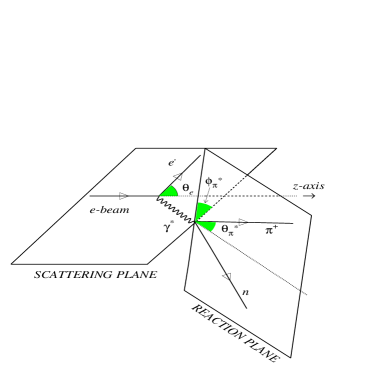
Figure 3: Kinematics of exclusive single $\pi^{+}$ electroproduction from a proton target.

A schematic illustration of electron scattering off a nucleon target producing an outgoing nucleon and one pion is shown in Fig. 3. The scattered electron angle $\theta_{e}$ is given in the laboratory frame. The angle between the virtual photon three-momentum and the direction of the pion is denoted as $\theta_{\pi}^{*}$ and the angle between the electron scattering plane and hadronic production plane is denoted as $\phi_{\pi}^{*}$. These two angles are defined in the center-of-mass frame of the hadronic system. The angle $\phi_{\pi}^{*}$ is defined so that the scattered electron lies in the $\phi_{\pi}^{*}=0^{\circ}$ half plane with the $z$-axis pointing along the virtual photon momentum. For exclusive single $\pi^{+}$ production from the proton, we request the simultaneous detection of one single electron and of one single $\pi^{+}$ in CLAS and the final state neutron will be identified by the missing mass squared $((p_{e}+p_{N})-(p_{e}^{\prime}+p_{\pi}))^{2}$, where $p_{\pi}$ is the four-momentum of the detected $\pi^{+}$. The kinematic range and bin sizes are chosen to provide reasonable statistics in each bin. These are summarized in Table 1.

Table 1: Kinematic bins used in this analysis.

Variable	Number of bins	Range		Bin size
$x_{B}$	7	$0.16$ - $0.58$		$0.06$
$Q^{2}$	5	$1.6$ - $3.1$ $\rm{GeV^{2}}$		$0.3$ $\rm{GeV^{2}}$
	3	$3.1$ - $4.5$ $\rm{GeV^{2}}$		$0.5$ $\rm{GeV^{2}}$
$-t$	6	$0.1$ - $1.9$ $\rm{GeV^{2}}$		$0.3$ $\rm{GeV^{2}}$
	3	$1.9$ - $4.3$ $\rm{GeV^{2}}$		$0.8$ $\rm{GeV^{2}}$
	1	$4.3$ - $5.3$ $\rm{GeV^{2}}$		$1.0$ $\rm{GeV^{2}}$

Our aim is to extract the three-fold differential cross section $\frac{1}{\Gamma}\frac{d^{3}\sigma}{dQ^{2}dx_{B}dt}$ where:

$$\frac{1}{\Gamma}\frac{d^{3}\sigma}{dQ^{2}dx_{B}dt}=\frac{n_{w}(Q^{2},x_{B},t)}{\mathcal{L}_{int}\ \Delta Q^{2}\ \Delta x_{B}\ \Delta t},$$ (1)

with

• $n_{w}(Q^{2},x_{B},t)$ is the weighted number of $ep\rightarrow e^{\prime}n\pi^{+}$ events in a given bin ($Q^{2}$, $x_{B}$, $t$); in particular, $n_{w}$ ($x_{B}$, $Q^{2}$, $-t$) contains the detector’s acceptance correction factor $Acc$($x_{B}$, $Q^{2}$, $-t$, $\phi^{*}_{\pi}$) (see Sec. 5.1) and the correction factor due to radiative effects $F_{rad}$($x_{B}$, $Q^{2}$, $-t$) (see Sec. 5.2),

• $\mathcal{L}_{int}$ is the effective integrated luminosity,

• $\Delta Q^{2}$, $\Delta x_{B}$ and $\Delta t$ are the corresponding bin widths (see Table 1); for bins not completely filled, because of $W$ or $E^{\prime}$ cuts on the electron for instance (see fig. 8), the phase space $\Delta Q^{2}\Delta x_{B}\Delta t$ includes a volume correction and the $Q^{2}$ and $x_{B}$ central values are modified accordingly.

In the following three sections, we detail the various cuts and correcting factors entering the definition of $n_{w}(Q^{2},x_{B},t)$.

4 Data Analysis

4.1 Particle identification and event selection

4.1.1 Electron identification

The electrons are identified at the trigger level by requiring at least 640 MeV energy deposited in the $\rm{EC}$ in coincidence with a signal in the $\rm{CC}$ (which triggers on one photoelectron).

Additional requirements for particle identification (PID) were used in the off-line analysis to refine the electron identification. First, we required that the $\rm{EC}$ and $\rm{CC}$ hits matched with a reconstructed track in the drift chambers ($\rm{DC}$). Second, we correlated the energy deposited in the $\rm{EC}$ and the momentum obtained by the track reconstruction in the $\rm{DC}$. This is aimed at removing the pion contamination. Electrons deposit energy in proportion to their incident energy in the calorimeter whereas pions are minimum ionizing and deposit a constant amount of energy in the calorimeter. The ratio of the total deposited energy in the $\rm{EC}$ to the momentum of the particle is called the sampling fraction. For electrons, approximately 30% of the total energy deposited in the $\rm{EC}$ is directly measured in the active scintillator material. The remainder of the energy is deposited in the lead sheets interleaved between the scintillators. Figure 4 shows the sampling fraction ${E}/{p_{e}}$ versus particle momentum $p_{e}$. The average sampling fraction for electrons was found to be 0.291 for this experiment. The solid lines in Fig. 4 show the $\pm$3$\sigma$ sampling fraction cuts used in this analysis.

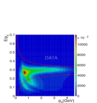
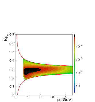
Figure 4: (color online). $\rm{EC}$ sampling fraction versus particle momentum for the experimental data before (top) and after (bottom) EC energy cuts. The solid curves show the $\pm 3\sigma$ sampling fraction cuts which are applied to select electrons.

To further reject pions, we required the energy deposited in the inner $\rm{EC}$ to be larger than $50$ MeV. Minimum ionizing particles lose less than this amount in the 15 cm thickness of the inner $\rm{EC}$.

Fiducial cuts were applied to exclude the $\rm{EC}$ detector edges. When an electron hit is close to an edge, part of the shower leaks outside the device; in this case, the energy cannot be fully reconstructed from the calorimeter information alone. This problem can be avoided by selecting only those electrons lying inside a fiducial volume within the $\rm{EC}$ that excludes the edges. A $\rm{GEANT}$-based simulation ($\rm{GSIM}$) was used to determine the $\rm{EC}$-response with full electron energy reconstruction. The calorimeter fiducial volume was defined by cuts that excluded the inefficient detector regions.

Particle tracks were reconstructed using the drift chamber information, and each event was extrapolated to the target center to obtain a vertex location. We demanded that the reconstructed $z$-vertex position (distance along the beam axis from the center of $\rm{CLAS}$, with negative values indicating upstream of the $\rm{CLAS}$ center) lies in the range $-80\;\rm{mm}<z_{\rm{vtx}}<-8\;\rm{mm}$. This is slightly larger than the target cell size in order to take into account the resolution effects on the vertex reconstruction.

Finally, a lower limit on the number of photoelectrons detected in the photomultiplier tubes of the $\rm{CC}$ provided an additional cut to improve electron identification. The number of photoelectrons detected in the $\rm{CC}$ follows a Poisson distribution modified for irregularities in light collection efficiency for the individual elements of the array. For this experiment, a good electron event was required to have 3 or more photoelectrons detected in the $\rm{CC}$. The efficiency of the $\rm{CC}$ cut was determined from the experimental data. We fit the number of photoelectrons using the modified Poisson distribution. The efficiency range after the $\rm{CC}$ cut is 78% to 99% depending on the kinematic region. The correction is then the integral below the cut divided by the total integral of the resulting fit function.

4.1.2 Positively charged pion identification

The main cuts to select the $\pi^{+}$ are based on charge, $z$-vertex, fiducial cuts and velocity versus momentum correlations. The velocity $\beta$ is calculated from the ratio of the path length of the reconstructed track, to the time of flight.

Figure 5 shows the $\beta$ versus $p$ distribution for positively charged particles from experimental data (top) and from the $\rm{GSIM}$ Monte Carlo simulation (bottom). A Gaussian is fit to $\beta$ for bins in momentum $p_{\pi}$. A $\pm 1.5\sigma$ cut on $\beta$ is chosen for pion candidates as shown in Fig. 5 (solid curves in the plot). Pions and positrons ($\beta=1$) are well separated below $p_{\pi}=250\;\rm{MeV/c}$ of momentum in the experimental data, but this is no longer the case at momenta larger than $400\;\rm{MeV/c}$. For this reason, positrons can be mis-identified as pions, which increases the background. At higher momenta, there can also be some particle mis-identification from protons and kaons. We estimated that the missing mass and vertex cuts reduce this mis-identification to the 5 - 10% level. This residual background contamination was subtracted as described in Sec. 6.

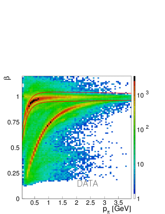
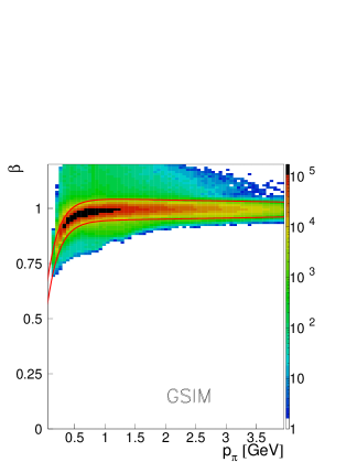
Figure 5: (color online). Velocity $\beta$ versus momentum for $\pi^{+}$ candidates using experimental data (top) and the $\rm{GSIM}$ Monte Carlo simulation (bottom). The solid curves are $\pm 1.5\sigma$ $\beta$ cut lines used to select $\pi^{+}$ from positron ($\beta$=1 band) and proton ($\beta<$0.8 band) backgrounds. (The data are issued from a skimmed file which selected one electron and at least one positively charged particle and one neutral particle).

4.2 Fiducial cuts

4.2.1 Electron fiducial cuts

The fiducial cuts for electrons were developed to exclude regions with non-uniform detector efficiency such as the edges of a sector in the $\rm{CC}$ and $\rm{EC}$. The fiducial cut is a function of the angles $\theta_{e}$, $\phi_{e}$, and momentum $p_{e}$ of the electron. An example of such fiducial cut can be seen in Fig. 6 for a given electron momentum bin. The solid line in the top plot shows the boundary of the fiducial region for the central momentum in that bin. Only electron events inside the curve (blue area) were used in the analysis. This curve was determined by selecting the flat high-efficiency areas in the $\theta_{e}$-sliced $\phi_{e}$ distributions. The histograms on the bottom of Fig. 6 show examples of such $\phi_{e}$ distributions at two values of $\theta_{e}=23^{\circ}\pm 0.5^{\circ}$ and $29^{\circ}\pm 0.5^{\circ}$. One sees a central, uniform area, flanked by two fringes. The highlighted area in the center indicates the selected fiducial range. In addition, a set of $\theta_{e}$ versus $p_{e}$ cuts was used to eliminate the areas with low detection efficiency due to problematic time-of-flight counters, photomultiplier tubes in Cherenkov counters, or drift chamber areas.

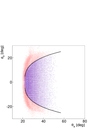
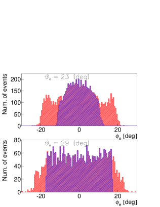
Figure 6: (color online). Example of electron fiducial cuts for the electron momentum bin ($p_{e}=1.437\;\pm.025\;\rm{GeV}$) in Sector 2. See the detailed explanation in the text.

4.2.2 Pion fiducial cuts

The fiducial cuts for pions depend on the angles $\theta_{\pi}$, $\phi_{\pi}$ and the momentum $p_{\pi}$. The pion momentum is scanned in $100\;\rm{MeV}$ steps from $0.3$ to $1.7\;\rm{GeV}$. The uniform detector efficiency region was determined by selecting a flat high-efficiency $\phi_{\pi}$ region in each $\theta_{\pi}$-sliced momentum bin, and the bad $\rm{TOF}$ counters and the inefficient $\rm{DC}$ areas were excluded by additional software cuts (the same procedure as was applied to electrons). Figure 7 shows an example for the fiducial cuts for pions. The low-efficiency $\rm{DC}$ regions (between the black solid lines) and the bad $\rm{TOF}$ paddles (between red solid lines) are removed in both experimental (top) and simulated (bottom) data as part of the fiducial cuts.

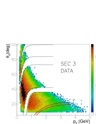
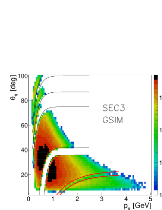
Figure 7: (color online). Pion polar angular distribution as a function of momentum in Sector 3. The low detector response areas are removed by empirical cuts for experimental (top) and simulated data (bottom). The black thin solid curves are fiducial cuts based on $\rm{DC}$ inefficiencies and the red thick solid curves are cuts for bad $\rm{TOF}$ counters.

4.3 Kinematic corrections

Due to effects that are not included in the reconstruction software (deviations of the magnetic field from perfect toroidal symmetry, misalignment of the tracking system,…), we have to apply some empirical corrections to the measured angles and momenta of both electrons and pions. For electrons, the kinematic corrections are applied using the elastic $ep\to e^{\prime}p^{\prime}$ process for which the kinematics is over-constrained. The goal is to correct the three-momentum of the electron so as to minimize the constraints due to the equations of conservation of energy and momentum. The same procedure is applied to the $\pi^{+}$’s three-momentum using our reaction $ep\to e^{\prime}\pi^{+}n$ under study, minimizing the deviation of the missing mass peak position from the neutron mass. The same correction factors are used for all events having the same kinematics. In this way we keep the spatial resolution of the drift chamber systems and multiple scattering effects and the missing mass resolution approaches its intrinsic limitations. The corrections were most sizable ($\approx$ 5%) for the pion momentum. They resulted in an improved missing mass resolution, from 23 to 35 MeV depending on kinematics. The corrections were most sizable for the high-momentum and forward-angle pions at high $W$ which are of interest in this experiment. We then applied additional ad-hoc smearing factors for the tracking and timing resolutions to the Monte Carlo so that they match the experimental data.

5 Monte Carlo simulation

In order to calculate the CLAS acceptance for $ep\to e^{\prime}\pi^{+}n$, we simulated electron and pion tracks using the CLAS $\rm{GEANT3}$-based Monte Carlo Package $\rm{GSIM}$. For systematic checks, we used two Monte Carlo event generators. Our approach is that by comparing the results of simulations carried out with two very different event generators, a conservative and reliable estimation of systematic effects, such as finite bin size effects, is obtained. The first event generator, $\rm{GENEV}$ (see Ref. genev for the original publication dedicated to photoproduction processes), generates events for various exclusive meson electroproduction reactions for proton and neutron targets ($\pi$, $\omega$, $\rho^{0}$, and $\phi$), including their decay, radiative effects, and resonant and non-resonant multi-pion production, with realistic kinematic distributions. $\rm{GENEV}$ uses cross section tables based on existing photoproduction data and extrapolates to electroproduction by introducing a virtual photon flux factor ($\Gamma$) and the electromagnetic form factors. Radiative effects, based on the Mo and Tsai formula MoTsai00 , are part of this event generator as an option. Although the formula is exact only for elastic $e$-$p$ scattering, it can be used as a first approximation to simulate the radiative tail and to estimate bin migration effects in our pion production process, as will be discussed in Sec. 5.2. The second event generator, $\rm{FSGEN}$ fsgen , distributes events according to the $ep\to e^{\prime}\pi^{+}n$ phase space.
Electrons and positive pions were generated under the “e1-6” experimental conditions. Events were processed through $\rm{GSIM}$. As already mentioned, additional ad-hoc smearing factors for the tracking and timing resolutions are applied after $\rm{GSIM}$ so that they match the experimental data. The low-efficiency regions in the drift chambers and problematic $\rm{TOF}$ channels were removed during this procedure. Acceptance and radiative corrections were calculated for the same kinematic bins as were used for the yield extraction as shown in Table 1. Figure 8 shows the binning in $Q^{2}$ and $x_{B}$ applied in this analysis. However, some bins will be dropped at some later stage in the analysis, in particular due to very low acceptances (see following subsection). Our cross sections will be defined at the ($x_{B},Q^{2},-t$) values given by the geometrical center of the three-dimensional bins. To account for non-linear variations of the cross section within a bin, a correction to our cross sections is determined by fitting with a simple ad-hoc three-variable function the simultaneous ($x_{B},Q^{2},-t$)-dependence of our cross sections. This correction comes out at the level of a couple of percent in average.

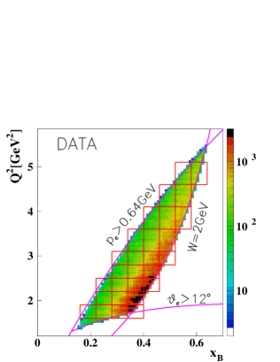
Figure 8: (color online). Kinematic coverage and binning (red boxes) as a function of $x_{B}$ and $Q^{2}$ (integrated over all other variables) for the experimental data. Only events with $W>2\;\rm{GeV}$ are shown.

5.1 Acceptance corrections

We related the experimental yields to the cross sections using the acceptance, including the efficiency of the detector. The acceptance factor ($Acc$) compensates for various effects, such as the geometric coverage of the detector, hardware and software inefficiencies, and resolution from track reconstruction. We generated approximately $850$ million events, taking radiative effects into account. This results in a statistical uncertainty for the acceptance determination of less than 5% for most bins, which is much lower than the systematic uncertainty that we have estimated (see Sec. 7).

We define the acceptance as a function of the kinematic variables,

$$Acc(x_{B},Q^{2},-t,\phi^{*}_{\pi})=\frac{N^{REC}(x_{B},Q^{2},-t,\phi^{*}_{\pi})}{N^{GEN}_{rad.}(x_{B},Q^{2},-t,\phi^{*}_{\pi})}~{},$$ (2)

where $N^{REC}$ is the number of reconstructed particles and $N^{GEN}_{rad.}$ is the number of generated particles in each kinematic bin (the meaning of the subscript $rad.$ will become clear in the next section). The kinematic variables in $N^{GEN}$ refer to the generated values so that bin migration effects are taken into account in the definition of our acceptance. The acceptances are in general between 1 and 9%. Figure 9 shows examples of acceptances, determined with the $\rm{GENEV}$+$\rm{GSIM}$ packages, as a function of the angle $\phi_{\pi}^{*}$ at a given $Q^{2}$ for various $x_{B}$ and $t$ bins. Bins with an acceptance below 0.2% were dropped. For the integration over the $\phi_{\pi}^{*}$ angle, in order to obtain our three-fold cross sections, we fitted the acceptance-corrected $\phi_{\pi}^{*}$ distributions, so that any hole in the $\phi_{\pi}^{*}$ distribution would be replaced by its fit value.

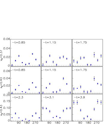
Figure 9: (color online). Examples of acceptance as a function of $\phi_{\pi}^{*}$ for various $t$ and $x_{B}$ bins at $Q^{2}=2.35\;\rm{GeV}^{2}$. The dips at $\phi_{\pi}^{*}$ = 0^∘ and 180^∘ are due to sector boundaries in $\rm{CLAS}$.

5.2 Radiative correction

Our goal is to extract the so-called Born cross section (tree-level) of the $p(e,e^{\prime}\pi^{+})n$ which can thus be compared to models. However, we measure a process which is accompanied by higher order radiative effects. Our experimental cross section must therefore be corrected. Radiative corrections are of two types: “virtual” corrections where there is no change in the final state of the $p(e,e^{\prime}\pi^{+})n$ process and “real” ones where there is in addition one (or several) Bremsstrahlung photon(s) in the final state. Such real Bremsstrahlung photons can originate either from the primary hard scattering at the level of the target proton (internal radiation) or from the interaction of the scattered or the initial electron with the various material layers of the $\rm{CLAS}$ detector that it crosses (external radiation).

We have dealt with these corrections in two steps. The effects of the radiation of hard photons (for instance, the loss of events due to the application of a cut on the neutron missing mass) are taken into account by the Monte Carlo acceptance calculation described in the previous section. Indeed, as mentioned earlier, the $\rm{GENEV}$ code has the option to generate radiative photons according to the Mo and Tsai formula and the $N^{GEN}_{rad.}$ events in Eq. 2 were generated with this option turned on. Figure 10 shows examples of the simulated neutron missing mass with and without radiative effects in two $W$ bins, obtained with the $\rm{GENEV}$ event generator and $\rm{GSIM}$. Again, the Monte Carlo simulations were carried out with the same cut procedures and conditions as used in the data analysis.

Then, the correction due to soft photons and virtual corrections is determined by extracting the ratio between the number of events without radiative and with radiative effects at the level of $\rm{GENEV}$ for each three-dimensional kinematic bin. We therefore apply the following additional correction factor to our data:

$$F_{rad}(x_{B},Q^{2},-t)=\frac{N^{GEN}_{norad.}(x_{B},Q^{2},-t)}{N^{GEN}_{rad.}(x_{B},Q^{2},-t)}.$$ (3)

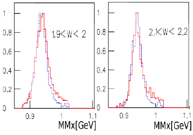
Figure 10: (color online). The simulated neutron missing mass distributions for two $W$ bins with $\Delta W=100\;\rm{MeV}$ at $W=1.95$ (left) and $2.15$ (right) $\;\rm{GeV}$ integrated over $\phi_{\pi}^{*}$, $\cos\theta_{\pi}^{*}$, and $Q^{2}$. Normalized yields are shown with (solid red) and without (dashed blue) radiative effects.

As a check, these radiative-correction factors were also calculated with the $\rm{EXCLURAD}$ code afanasev , which contains a complete description of all internal radiative effects in exclusive processes, but is currently valid only up to $W=2\;\rm{GeV}$. We compare the two different radiative-correction methods in a kinematic region where both methods are valid. Figure 11 shows the results for radiative-correction factors in the region $W\approx 1.75\;\rm{GeV}$ and $Q^{2}\approx 3\;\rm{GeV}^{2}$ as a function of $\cos\theta^{*}_{\pi}$.

The radiative correction factors from $\rm{EXCLURAD}$ are within $\pm 20\%$ of unity over the full $\cos\theta_{\pi}^{*}$ range (red solid points). The radiative corrections from $\rm{GENEV}$+$\rm{GSIM}$ also fluctuate around $1.0$ with a similar structure (blue open circles). The $\rm{GENEV}$+$\rm{GSIM}$ error bars are due to Monte Carlo statistics ($\rm{EXCLURAD}$ is a theoretical code which has therefore no statistical uncertainty). The agreement between the two approaches is important because $\rm{EXCLURAD}$ is believed to be the most reliable of the two methods because it does not have the limitations of Mo and Tsai. Building on this reasonable agreement in this part of the phase space, we rely on the $\rm{GENEV}$+$\rm{GSIM}$ radiative-correction factors for our data. In Sec. 7, we discuss the systematic uncertainty associated with these radiative corrections.

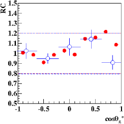
Figure 11: (color online). Radiative-correction factors (RC) as a function of $\cos\theta_{\pi}^{*}$ from $\rm{EXCLURAD}$ (red solid points) at $W=1.74\;\rm{GeV}$, $Q^{2}=3\;\rm{GeV^{2}}$, and $\phi_{\pi}^{*}=112.5^{\circ}$ and $\rm{GENEV}$ plus $\rm{GSIM}$ (blue open circle) at $W\approx 1.75\;\rm{GeV}$, $Q^{2}\approx 3\;\rm{GeV}^{2}$, and $80^{\circ}<\phi_{\pi}^{*}<120^{\circ}$.

6 Background subtraction

There are two main sources of background in our reaction. One consists of the mis-identification of pions with other positively charged particles (protons, kaons, positrons). This is particularly important for the pion-proton separation at high-momenta ($p>2\;\rm{GeV}$), see Sec. 4.1. The other consists of multi-pion production. To subtract both backgrounds, we fit the neutron missing mass distribution bin by bin. We used many methods to fit these spectra: fit of only the background, fit of the signal plus background, with different functional forms both for the signal and the background, variation of the fitted range, etc… from which we extracted a systematic uncertainty (see Sec. 7).

Figure 12 (top) shows an example of a fit based on only the background, with an exponential plus a Gaussian. The former function was determined from simulations of the multi-pion spectra in the neutron missing mass region $>1.02\;\rm{GeV}$. A comparison of the missing mass ($\rm{MMx}$) spectrum is shown in the bottom plot of Fig. 12 before (black squares) and after (red solid circles) background subtraction. In the range of the neutron missing mass cut, shown by the two vertical lines at $0.877\;\rm{GeV}$ and $1.0245\;\rm{GeV}$, the background is small, and the remaining radiative tail becomes visible after the background is subtracted.

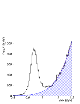
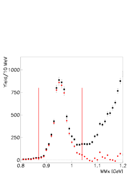
Figure 12: (color online). Example of the missing mass peak plus background at $Q^{2}=2.65\;\rm{GeV}^{2}$, $-t=1.15\;\rm{GeV^{2}}$, and $x_{B}=0.43$. The top plot shows the fitted background distribution (hashed region). The bottom plot shows the neutron missing mass distribution before (black squares) and after (red solid points) background subtraction.

7 Systematic uncertainties

Several sources of systematic uncertainty that can affect our measurements have been studied by changing various cuts and using different event generators.

We varied the criteria used for the particle identification to provide more and less stringent particle selection simultaneously for experimental and GSIM data and then reran the complete analysis. The cuts on $\rm{EC}$ energy deposition and $\rm{CC}$ amplitude for the electron, as well as cuts on the $\rm{TOF}$ timing for the pion, have been varied. The $\rm{EC}$ sampling fraction cut was varied from $\pm 3\sigma_{\rm{EC}}$ to $\pm 2\sigma_{\rm{EC}}$ which led to a 5% uncertainty for electron identification. Changing the $\rm{TOF}$ $\beta$ cut from $\pm 2\sigma_{\rm{TOF}}$ to $\pm 2.5\sigma_{\rm{TOF}}$ for pion identification gives a 1.7% uncertainty. The various cuts for channel identification such as fiducial, missing mass, and vertex cuts produced 3%, 1%, and 1.6% systematic uncertainties, respectively.

Acceptance and radiative corrections are the biggest sources of systematic errors. The systematic uncertainty from the acceptance is evaluated by comparing our results using the $\rm{GENEV}$ and $\rm{FSGEN}$ event generators. In the limit of infinitely large statistics and infinitely small bin size, our acceptances should be model-independent (up to the bin-migration effects). But these conditions are not reached here and we find differences between 2 and 8%. The systematic uncertainty for radiative corrections is estimated similarly by comparing the radiative-correction factors ($\rm{GENEV}$ and $\rm{EXCLURAD}$). We calculated the difference between the cross sections corrected for radiative effects using either $\rm{GENEV}$-$\rm{GEANT}$ simulation or the $W$-expanded $\rm{EXCLURAD}$ (where $\rm{EXCLURAD}$ was linearly extrapolated to $W>2$ GeV). An average $8\%$ systematic uncertainty was found. Acceptance and radiative corrections are actually correlated, but after a combined analysis we estimated an averaged range $4-12\%$ total uncertainty for both of these effects together.

Concerning the background subtraction procedure under the neutron missing mass (see Sec. 6), we used various fitting functions (Gaussian plus exponential, Gaussian plus polynomial, exponential plus polynomial, etc.) and various fitting ranges. These various fitting functions and ranges eventually produced small differences and we estimated a 3$\%$ systematic uncertainty associated with this procedure.

To take into account the model-dependency of our bin-centering correction (see Sec. 4.3), we also introduce an error equal to the correction factor itself which is, we recall, at the level of a couple of percent in average.

These latter systematic uncertainties were determined for each bin. Concerning overall scale uncertainties, the target length and density have a 1% systematic uncertainty and the integrated charge uncertainty is estimated at 2%. The background from the target cell was subtracted based on the empty-target runs and amounted to 0.6$\pm$0.2% of our $e^{\prime}\pi^{+}X$ events. The total systematic uncertainties, averaged over all bins, is then approximately 12%. Table 2 summarizes the main systematic uncertainties in this analysis averaged over all the accessible kinematic bins seen in Fig. 8.

Table 2: Average systematic uncertainties for the differential cross sections.

Source	Criterion	Estimated
		contribution
Type	point-to-point
$e^{-}$ PID	sampling fraction
	cut in $\rm{EC}$
	($3\sigma_{\rm{SF}}\to 2\sigma_{\rm{SF}}$)	5%
$e^{-}$ fiducial cut	fiducial volume change
	($10\%$ reduced)	2.5%
${\pi}^{+}$ PID	$\beta$ resolution change
	($2\sigma_{\rm{TOF}}\to 2.5\sigma_{\rm{TOF}}$)	1.7%
${\pi}^{+}$ fiducial cut	width ($10\%$ reduced)	3.5%
Missing	neutron missing
mass	mass resolution
cut	($3\sigma_{\rm{MMx}}\to 3.5\sigma_{\rm{MMx}}$)	1%
Vertex cut	$z$-vertex width
	($5\%$ reduced)	1.6%
Acceptance	$\rm{GENEV}$ vs $\rm{FSGEN}$
Radiative	$\rm{GENEV}$ vs $\rm{EXCLURAD}$	4-12%
corrections
Background	various fit functions
subtraction	exponential, gaussian
	and high order polynomials	3%
Bin-centering	toy model	2-4%
effect
Type	overall scale/normalization
LH2 target	density/length	1%
Luminosity	integrated charge	2%
Total		9-14%

8 Results and Discussion

In this section, we present our results for the cross sections of the $p(e,e^{\prime}\pi^{+})n$ reaction in the invariant mass region $W>2\;\rm{GeV}$. We have extracted the differential cross sections as a function of several variables ($t$, $Q^{2}$, and $W$ or $x_{B}$). The angle $\phi^{*}_{\pi}$ is always integrated over in the following. The extraction of the interference cross sections $\sigma_{TT}$ and $\sigma_{TL}$ is the subject of an ongoing analysis and will be presented in a future article. The error bars on all cross sections include both statistical and systematic uncertainties added in quadrature. All values of our cross sections and uncertainties can be found on the CLAS database web page: http://clasweb.jlab.org/cgi-bin/clasdb/db.cgi

8.1 ${d\sigma}/{dt}$ as a function of $t$

Fig. 13 shows the differential cross section ${d\sigma}/{dt}$ as a function of $t$ for different ($x_{B}$, $Q^{2}$) bins. We define the reduced differential cross section:

$$\frac{d\sigma}{dt}=\frac{1}{\Gamma}\frac{d^{3}\sigma}{dQ^{2}dx_{B}dt}~{},$$ (4)

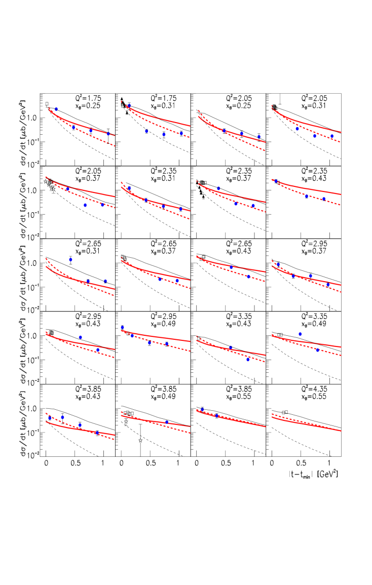
Figure 14: (color online). Same as Fig. 13 except with an expanded low $|t-t_{min}|$ scale, where -$t_{min}$ is the minimum kinematically possible four-momentum transfer. In addition, the black solid triangles HPBlok show the $\rm{JLab}$ $\rm{Hall~{}C}$ extracted $d\sigma_{L}/dt$ data.

where the virtual photon flux factor Hand has been factored out. We have included in Fig. 13 the $\rm{JLab}$ $\rm{Hall~{}C}$ data, which cover only the very small $t$ domain. We note that there is generally reasonable agreement between the results of the two experiments. However, care must be taken in comparing the Hall C and Hall B measurements as the central ($t$, $Q^{2}$, and $W$ or $x_{B}$, $\epsilon$) values do not exactly match each other. For instance, the most important discrepancy seems to appear in the bin ($x_{B}$, $Q^{2}$)=(0.49, 3.35) where the Hall C measurement was carried out at $\epsilon$=0.45 XQian while ours corresponds to $\epsilon$=0.58 (the $x_{B}$ and $Q^{2}$ values being almost similar). According to the value of $\sigma_{L}$ relative to $\sigma_{T}$, the Hall C cross section should then be renormalized: by a factor of 1.58/1.45$\approx$10% (if $\sigma_{L}$$\approx$$\sigma_{T}$ which the Hall C separated data Horn09 ; HPBlok indicate, although at a slightly different kinematics) to a factor 0.58/0.45$\approx$30% (if $\sigma_{L}$ dominates over $\sigma_{T}$ which the Laget model predicts). For better visualization, which is also relevant for the comparison with the models, we also show Fig. 14 which concentrates on the low $|t|$ range of Fig. 13.

The ${d\sigma}/{dt}$ cross sections fall as $|t|$ increases, with some flattening at large $|t|$, which is a feature that is also observed in photoproduction RAnderson00 ; LYZhu . For several bins, for instance ($x_{B}$, $Q^{2}$)=(0.31, 1.75) or (0.37, 2.05), we notice a structure in ${d\sigma}/{dt}$ for $|t|\approx$ 0.5 GeV². The origin of this dip is not known. We note that the $\rm{JLab}$ $\rm{Hall~{}C}$ experiment XQian also measured such a structure in ${d\sigma}/{dt}$ (see Fig. 13 in Ref. XQian for bin ($W$, $Q^{2}$)=(1.8, 2.16)).

We first compare our data to calculations using hadronic degrees of freedom. The first one with which we will compare our data is the Laget model JMLaget01 based on Reggeized $\pi^{+}$ and $\rho^{+}$ meson exchanges in the $t-$channel VGL . The hadronic coupling constants entering the calculation are all well-known or well-constrained, and the main free parameters are the mass scales of the electromagnetic form factors at the photon-meson vertices.

If one considers only standard, monopole, $Q^{2}$-dependent form factors, one obtains much steeper $t$-slopes than the data. An agreement with the data can be recovered by introducing a form factor mass scale that also depends on $t$ according to the prescription of Ref. JMLaget01 . This form factor accounts phenomenologically for the shrinking in size of the nucleon system as $t$ increases. The size of the effect is quantitatively the same as in the $p(e,e^{\prime}\omega)p$ channel (see Fig. 1 of Ref. JMLaget01 ), which is dominated by pion exchange in the same energy domain as in our study. The results of this calculation with ($Q^{2}$, $t$)-dependent meson electromagnetic form factors are shown, for ${d\sigma_{L}}/{dt}$ and ${d\sigma}/{dt}={d\sigma_{T}}/{dt}+\epsilon{d\sigma_{L}}/{dt}$, in Figs. 13 and 14 by the red curves. The Laget model gives a qualitative description of the data, with respect to the overall normalization at low $t$ and the $x_{B}$-, $Q^{2}$- and $t$- dependencies. We recall that this model already gives a good description of the photoproduction data ($\rm{SLAC}$, $\rm{JLab}$) and of the $\rm{HERMES}$ electroproduction data, and that the form factor mass scale JMLaget01 has not been adjusted to fit our data.

In the framework of this model, ${d\sigma_{L}}/{dt}$ dominates at low $|t|$, while ${d\sigma_{T}}/{dt}$ takes over around $|t|\approx$ 2 GeV², this value slightly varying from one ($Q^{2}$, $x_{B}$) bin to another. This dominance of $\sigma_{L}$ at low $|t|$ is a consequence of the $t$-channel $\pi^{+}$-exchange (pion pole). At larger $|t|$, the $\rho^{+}$ meson exchange, which contributes mostly to the transverse part of the cross section, begins to dominate. The Laget Regge model, in addition to $t$-channel meson exchanges, also contains $u$-channel baryon exchanges. It thus exhibits an increase of the cross section in some ($Q^{2}$, $x_{B}$) bins at the largest $|t|$-values, corresponding to low-$|u|$ values. We have additional data at larger $|t|$ (lower $|u|$) that are currently under analysis.

The second model with which we compare our data is the “hybrid” two-component hadron-parton model proposed in Refs. Kaskulov:2008xc ; Kaskulov:2009gp . Like in the Laget model, it is based on the exchange of the $\pi^{+}$ and $\rho^{+}$ Regge trajectories in the $t$-channel. However, the model complements these hadron-like interaction types, which dominate in photoproduction and low $Q^{2}$ electroproduction, by a direct interaction of virtual photons with partons at high values of $Q^{2}$ followed by string (quark) fragmentation into $\pi^{+}n$. The partonic part of the production mechanism is described by a “deep inelastic”-like electroproduction mechanism where the quark knockout reaction $\gamma^{*}q\to q$ is followed by the fragmentation process of the Lund type. The transverse response is then treated as the exclusive limit of the semi-inclusive reaction $p(e,e^{\prime}\pi^{+})X$. Figures 13 and 14 show the results of this model compared to our data where very good agreement is found. This calculation was also found to give a good description of the L/T-separated Hall C and unseparated HERMES data Kaskulov:2008xc ; Kaskulov:2009gp .

The third model that we wish to discuss, the GK model, is based purely on partonic degrees of freedom and is based on the handbag GPD formalism. In this model ${d\sigma_{L}}/{dt}$ is also mostly generated by the pion pole, similar to the two previous models. There are, however, a couple of differences in the treatment of this pion pole in the GK calculation. For instance, the Laget model has an intrinsic energy dependence. It is “Reggeized”, so the $t$-channel propagator is proportional to $s^{\alpha_{\pi}(t)}$, where $\alpha_{\pi}(t)$ is the pion Regge trajectory. In addition, it uses a ($Q^{2}$, $t$)-dependent electromagnetic form factor. These two features change the $s$-, $x_{B}$-, and $t$- dependencies of the pion pole with respect to the GK treatment. Indeed, in the latter case, the $t$-channel pion propagator is proportional to ${1}/{(t-m^{2}_{\pi})}$, so it has no s-dependence, and the hadronic form factor at the $\pi NN$ vertex is only $t$-dependent.

Figure 15 shows the results of the GK calculation (in blue) for ${d\sigma_{L}}/{dt}$ and ${d\sigma}/{dt}$. We recall that the GK model is applicable only for small values of $-t/Q^{2}$. Outside this regime, higher-twist contributions that are not taken into account in the GK handbag formalism are expected. The GK model describes qualitatively our low-$t$ unseparated cross sections over our whole ($x_{B}$, $Q^{2}$) domain. This is remarkable since the GK model was optimized for higher-energy kinematics ($\rm{HERMES}$) and no further adjustments were made for the present $\rm{CLAS}$ kinematics. We see that ${d\sigma_{L}}/{dt}$ has a non-negligible contribution only in the very low $|t|$ domain and only for a few ($x_{B}$, $Q^{2}$) bins, in particular at the lowest $x_{B}$ and the largest $Q^{2}$ values (for instance, the ($x_{B}$, $Q^{2}$) bins (0.25, 1.75) and (0.31, 2.35)). This is in line with the observation that at $\rm{HERMES}$ kinematics, i.e. at lower $x_{B}$ and larger $Q^{2}$ values, the longitudinal part of the cross section dominates in the GK model at low $|t|$. For the larger $x_{B}$ values, one sees that the dominance of ${d\sigma_{L}}/{dt}$ at low $|t|$ is not at all systematic in the GK calculation. The ratio of ${d\sigma_{L}}/{dt}$ to ${d\sigma}/{dt}$ strongly depends on $x_{B}$. Specifically, it decreases as $x_{B}$ increases and at $x_{B}$=0.49, ${d\sigma_{L}}/{dt}$ is only a few percent of ${d\sigma}/{dt}$, even at the lowest $t$ values. This is a notable difference from the Laget Regge model for instance.

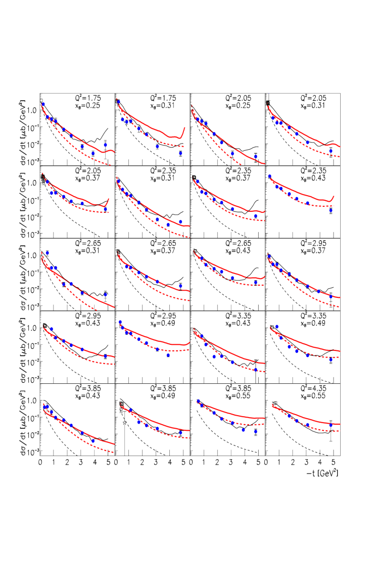
Figure 13: (color online). Differential cross sections $d\sigma/dt~{}[\mu b/\rm{GeV^{2}}]$ integrated over ${\phi^{*}_{\pi}}$ for various ($Q^{2}$, $x_{B}$) bins. The blue solid points are the present work. The error bars (outer error) on all cross sections include both statistical (inner error) and systematic uncertainties added in quadrature. The black open squares ($d\sigma/dt$) XQian and open stars ($d\sigma_{L}/dt$) Horn09 are $\rm{JLab}$ $\rm{Hall~{}C}$ data. The red thick solid ($d\sigma/dt$), and dashed ($d\sigma_{L}/dt$) curves are the calculations from the Laget model JMLaget01 with ($Q^{2},t$)-dependent form factors at the photon-meson vertex. The black thin solid ($d\sigma/dt$) and dashed ($d\sigma_{L}/dt$) curves are the calculations from the Kaskulov et al. model Kaskulov:2008xc . This model does not provide the calculation at ($x_{B}$, $Q^{2}$)=(0.43, 2.35), (0.49, 2.95) due to the kinematic limit in the model.

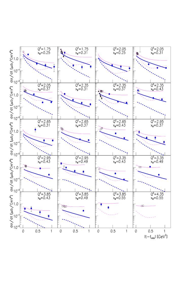
Figure 15: (color online). Same as Fig. 14 except with $|t-t_{min}|$ scale. The blue thick solid and dashed curves are $d\sigma$/$dt$ and $d\sigma_{L}$/$dt$, respectively, from the GK model GK11 . The magenta thin solid ($d\sigma/dt$) and dashed ($d\sigma_{L}/dt$) curves are the calculations from the 2nd Kaskulov et al. model Kaskulov:2010kf .

In particular, one can remark in Fig. 15, where we display in two ($x_{B}$, $Q^{2}$) bins ((0.31, 1.75) and (0.37, 2.35)) the longitudinal part of the cross section as extracted from Hall C HPBlok , that the longitudinal part of the GK calculation is not in good agreement with the experimental data. This can be attributed to the way the pion pole and/or the pion-nucleon form factor, which are the main contributors to the longitudinal part of the cross section, are modeled in the GK approach. A Reggeization (like in the Laget model) or a change in the pion-nucleon form factor parametrization could possibly enhance the pion pole contribution at JLab kinematics and provide better agreement with our data (without damaging the agreement with the HERMES data) private_kroll . We recall that the GK model for which the GPD parameters were fitted to the low $x_{B}$ HERMES data, was simply extrapolated to the kinematics of the present article without any optimization and thus the present disagreement observed in ${d\sigma_{L}}/{dt}$ should not be considered as definitive.

In the GK model, the transverse part of the cross section is due to transversity GPDs. In Fig. 15, the GK calculation predicts that the transverse part of the cross section dominates essentially everywhere in our kinematic domain. Although the GK L/T ratio probably needs to be adjusted as we just discussed, the GK calculation opens the original and exciting perspective to access transversity GPDs through exclusive $\pi^{+}$ electroproduction.

Finally, at the kinematics of our experiment, in spite of our $W>2$ GeV cut, it cannot be excluded that nucleon resonances contribute. In Ref. Kaskulov:2010kf , Kaskulov and Mosel identify these high-lying resonances with partonic excitations in the spirit of the resonance-parton duality hypothesis and invoke the continuity in going from an inclusive final deep inelastic state to exclusive pion production. During this transition one expects that the inclusion of resonance excitations enhances the transverse response while leaving the longitudinal strength originating in the $t$-channel meson exchanges intact. Thus, in this work, the $t$-channel exchange part of the production amplitude is again described by the exchange of the Regge trajectories ($\pi^{+}$, $\rho^{+}$ and $a_{1}^{+}$) to which it is added a nucleon resonance component that is described via a dual connection between the resonance and partonic deep inelastic processes. The parameters of this model have been tuned using the forward JLab Hall C data. Figure 15 shows the results of this calculation with our data and a reasonable agreement is found.

The four models that we just discussed, although they give a reasonable description of the unseparated cross sections, display rather different L/T ratios. The precise measurement of this ratio as a function of $x_{B}$, $Q^{2}$ and $t$ appears thus as essential to clarify the situation. For instance, in order to validate and/or tune the GK approach, it would be interesting to study the $Q^{2}$-dependence at fixed $x_{B}$ and $t$ of the longitudinal and transverse cross sections. They should approach, as $Q^{2}$ increases, a ${1}/{Q^{6}}$ and ${1}/{Q^{8}}$ scaling behavior respectively, as mentioned in the introduction of this article. In contrast, the Laget Regge model, for which $x_{B}$ is not a “natural” variable (it is rather $W$) should not predict such a $Q^{2}$ scaling at fixed $x_{B}$. Although we are probably very far from such an asymptotic regime, the measurement of the $Q^{2}$-dependence in the transition region accessible with the upcoming $\rm{JLab}$ 12-GeV upgrade should provide some strong constraints and in particular some checks on the way the higher-twist corrections are treated in the GK model. Such a program is already planned at JLab hallc-12gevprop .

8.2 ${d\sigma}/dt$ as a function of $Q^{2}$ at fixed $t$

Figures 16 and  17 show the differential cross section $d\sigma$/$dt$ as a function of $Q^{2}$ at fixed $x_{B}$ for various $t$ values. In Fig. 16, our data are fitted with a $1/Q^{n}$ function and are compared to the GK model. We recall that, at asymptotically large $Q^{2}$, the handbag mechanism predicts a dominance of $\sigma_{L}$ which should scale as ${1}/{Q^{6}}$ at fixed $t$ and $x_{B}$. The resulting exponents $n$ of our fit indicates a flatter $Q^{2}$ dependence than $1/Q^{6}$. At the relatively low $Q^{2}$ range accessed in this experiment, higher-twist effects are expected to contribute and hence the leading-twist ${1}/{Q^{6}}$ dependence of $\sigma_{L}$ is no longer expected. We note that such higher-twist contributions are part of the GK calculation and the GK model also does not show this scaling behavior at the present $Q^{2}$ values. Although the GK model tends to underestimate the normalization of our data, its $Q^{2}$ dependence agrees reasonably well with our data.

In Fig. 17, we compare our data to the Laget JMLaget01 and the Kaskulov et al. Kaskulov:2008xc ; Kaskulov:2009gp models. The Laget calculation gives a reasonable description of the data although it seems to have a slightly steeper $Q^{2}$-dependence than our data (particularly in the $x_{B}$=0.37 bin). We note that in the $x_{B}$=0.43 bin, our data seem to display a structure (dip) for $Q^{2}$ values between 3 and 4 GeV², which is certainly intriguing. We have at this stage no particular explanation for this. We just observe that the “hybrid” two-component hadron-parton model of Refs. Kaskulov:2008xc ; Kaskulov:2009gp displays apparently also such structure which should therefore be further investigated.

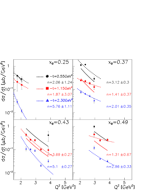
Figure 16: (color online). Differential cross sections $d\sigma/dt\;[\rm{\mu b/GeV^{2}}]$ versus $Q^{2}$ at fixed $x_{B}$ for various $t$ values. The dashed curves are the results of a fit to the function $A/Q^{n}$. The solid curves are the results of the GK calculations GK11 . The GK calculations are only valid for $-t<\;\approx 1$ GeV² so we do not display those results for $-t=2.3$ GeV².

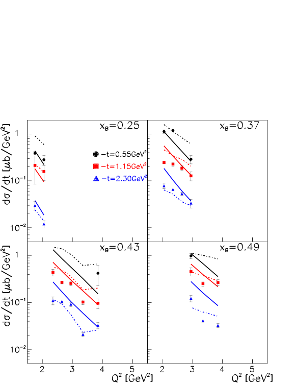
Figure 17: (color online). Differential cross sections $d\sigma/dt\;[\rm{\mu b/GeV^{2}}]$ versus $Q^{2}$ at fixed $x_{B}$ for various $t$ values. The solid curves are the results of the Laget calculations JMLaget01 and the dash-dotted curves of the “hybrid” two-component hadron-parton model of Refs. Kaskulov:2008xc ; Kaskulov:2009gp .

8.3 ${d\sigma}/{dt}$ as a function of $W$ at fixed $\theta_{\pi}^{*}$

Figure 18 shows our scaled cross sections, $s^{7}d\sigma/dt$, as a function of $W$ for four $Q^{2}$ values and four bins in $\cos\theta_{\pi}^{*}$: $-0.01\pm 0.16$, $0.27\pm 0.1$, $0.42\pm 0.05$ and $0.53\pm 0.06$. The lever arm in $W$ is limited. At $\theta_{\pi}^{*}=90^{\circ}$, where the scaling behavior is expected to set in most quickly, we have only 2 or 3 data points in $W$, depending on the $Q^{2}$ bin. It is therefore difficult to draw precise conclusions at this stage for the $W$-dependence at fixed $Q^{2}$. Nevertheless, with these limited (but unique) data, one can say that, at $\theta_{\pi}^{*}=90^{\circ}$, except for the 3 data points at $Q^{2}$=2.35 GeV², the $W$-dependence of $s^{7}{d\sigma}/{dt}$ does not appear to be constant. We also display in Fig. 18 the result of the Laget model. It gives, within a factor two, a general description of these large-angle data. The $W$-dependence of our data is very similar to the energy dependence that was observed in photoproduction WChen . In the same energy range as covered by the present study, real-photon data exhibit strong deviations from scaling. Within the Laget model, these deviations are accounted for by the coupling between the $n\pi^{+}$ and the $\rho N$ channels JML2010 . The $\rm{JLab}$ 12-GeV upgrade will allow us to increase the coverage in $W$ and check whether the hints of oscillations that we observe remain in the virtual-photon sector.

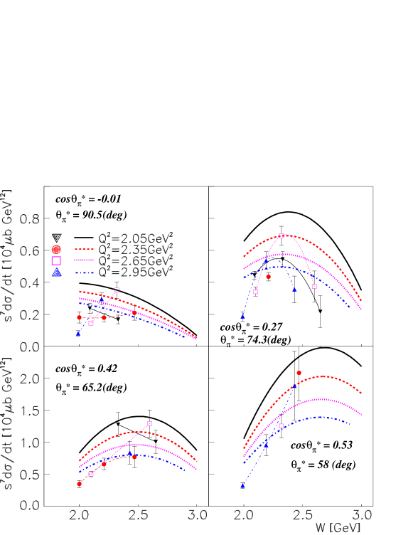
Figure 18: (color online). Scaled cross sections $s^{7}d\sigma/dt$ $[10^{4}\rm{\mu b}\;\rm{GeV^{12}}]$ versus $W$ for $\theta_{\pi}^{*}\approx$ 60${}^{\circ}\ldots$ 90^∘ and various $Q^{2}$ bins. Thick curves are from the Laget model JMLaget01 . The thin curves are to guide the eye, connecting points with the same $Q^{2}$ values.

9 Summary

We have measured the cross sections of exclusive electroproduction of $\pi^{+}$ mesons from protons as a function of $-t=0.1$ - $5.3\;\rm{GeV^{2}}$, $x_{B}=0.16$ - $0.58$, and $Q^{2}=1.6$ - $4.5\;\rm{GeV^{2}}$. We have compared our differential cross sections to four recent calculations based on hadronic and partonic degrees of freedom. The four models give a qualitative description of the overall strength and of the $t$-, $Q^{2}$- and $x_{B}$- dependencies of our unseparated cross sections. There is an obvious need for L-T separated cross sections in order to distinguish between the several approaches. These separations will be possible with the upcoming JLab 12-GeV upgrade. In particular, if the handbag approach can accomodate the data, the $p(e,e^{\prime}\pi^{+})n$ process offers the outstanding potential to access transversity GPDs.

10 Acknowledgment

We acknowledge the outstanding efforts of the staff of the Accelerator and the Physics Divisions at Jefferson Lab that made this experiment possible. We also give many thanks to P. Kroll, S. Goloskokov and M. Kaskulov for their calculations. The early work of D. Doré on this analysis is also acknowledged. This work was supported in part by the US Department of Energy, the National Science Foundation, the Italian Istituto Nazionale di Fisica Nucleare, the French American Cultural Exchange (FACE) and Partner University Funds (PUF) programs, the French Centre National de la Recherche Scientifique, the French Commissariat à l’Energie Atomique, the United Kingdom’s Science and Technology Facilities Council, the Chilean Comisión Nacional de Investigación Científica y Tecnológica (CONICYT), and the National Research Foundation of Korea. The Southeastern Universities Research Association (SURA) operated the Thomas Jefferson National Accelerator Facility for the US Department of Energy under Contract No.DE-AC05-84ER40150.

References

- (1) R. L. Anderson et al., Phys. Rev. D 14, 679 (1976); C. White et al., Phys. Rev. D 49, 58 (1994).
- (2) W. Chen et al., Phys. Rev. Lett. 103, 012301 (2009).
- (3) C. J. Bebek et al., Phys. Rev. D 13, 25 (1976).
- (4) C. J. Bebek et al., Phys. Rev. D 13, 1693 (1978).
- (5) T. Horn et al., Phys. Rev. C 78, 058201 (2008).
- (6) H. P. Blok et al., Phys. Rev. C 78, 045202 (2008).
- (7) X. Qian et al., Phys. Rev. C 81, 055209 (2010).
- (8) A. Airapetian et al., Phys. Lett. B 659, 486 (2008).
- (9) D. Müller, D. Robaschik, B. Geyer, F.-M. Dittes, and J. Hoeji, Fortschr. Phys. 42, 101 (1994).
- (10) X. Ji, Phys. Rev. Lett. 78, 610 (1997); Phys. Rev. D 55, 7114 (1997).
- (11) A.V. Radyushkin, Phys. Lett. B 380 (1996) 417; Phys. Rev. D 56, 5524 (1997).
- (12) J. C. Collins, L. Frankfurt, and M. Strikman, Phys. Rev. D 56, 2982 (1997).
- (13) S. V. Goloskokov and P. Kroll, Eur. Phys. J. C 65, 137 (2010).
- (14) S. J. Brodsky and G. P. Lepage, Phys. Rev. D 22, 2157 (1980).
- (15) S. J. Brodsky and G. R. Farrar, Phys. Rev. Lett. 31, 1153 (1973); Phys. Rev. D 11, 1309 (1975); V. Matveev et al., Nuovo Cimento Lett. 7, 719 (1973).
- (16) M. Vanderhaeghen, P. A. M Guichon, and M. Guidal, Phys. Rev. D 60, 094017 (1999).
- (17) S. V. Goloskokov and P. Kroll, Eur. Phys. J. A 47, 112 (2011).
- (18) L. Mankiewicz, G. Piller and A. Radyushkin, Eur. Phys. J. C 10, 307 (1999).
- (19) L. Frankfurt, P. Pobylitsa, M. Poliakov, and M. Strikman, Phys. Rev. D 60, 014010 (1999).
- (20) L. Y. Zhu et al., Phys. Rev. Lett. 91, 022003 (2003), Phys. Rev. C 71, 044603 (2005).
- (21) J. Napolitano et al., Phys. Rev. Lett. 61, 2530 (1988); S. J. Freedman et al., Phys. Rev. C 48, 1864 (1993); J. E. Belz et al., Phys. Rev. Lett. 74, 646 (1995).
- (22) C. Bochna et al., Phys. Rev. Lett. 81, 4576 (1998).
- (23) E. C. Schulte et al., Phys. Rev. Lett. 87, 102302 (2001).
- (24) P. Rossi et al., Phys. Rev. Lett. 94, 012301 (2005); M. Mirazita et al., Phys. Rev. C 70, 014005 (2004).
- (25) R. A. Schumacher and M. M. Sargsian, Phys. Rev. C 83, 025207 (2011).
- (26) B.A. Mecking et al., Nucl. Instrum. Methods A 51, 409 (1995).
- (27) K. Park et al., Phys. Rev. C 77, 015208 (2008).
- (28) P. Corvisiero et al., Nucl. Instrum. Methods A 346 433 (1994) and E. Golovach, M. Ripani, M. Battaglieri, R. De Vita, private communication.
- (29) L. W. Mo, Y. S. Tsai, Rev. Mod. Phys. 41, 205 (1969).
- (30) S. Stepanyan, private communication.
- (31) A. Afanasev et al., Phys. Rev. D 66, 074004 (2002).
- (32) L. Hand, Phys. Rev. 129, 1834 (1963).
- (33) J. M. Laget, Phys. Rev. D 70, 054023 (2004).
- (34) M. Guidal, J. M. Laget and M. Vanderhaeghen, Nucl. Phys. A 627, 645 (1997), Phys. Lett. B 400, 6 (1997).
- (35) M. M. Kaskulov, K. Gallmeister and U. Mosel, Phys. Rev. D 78, 114022 (2008).
- (36) M. M. Kaskulov and U. Mosel, Phys. Rev. C 80, 028202 (2009).
- (37) P. Kroll, private communication.
- (38) M. M. Kaskulov and U. Mosel, Phys. Rev. C 81, 045202 (2010).
- (39) T. Horn et al., Jefferson Lab E12-07-105, http://www.jlab.org/exp_prog/proposals/07/PR12-07-105.pdf.
- (40) J. M. Laget, Phys. Lett. B 685, 146 (2010).