Generating and Adding Flows on Locally Complete Metric Spaces

Abstract

As a generalization of a vector field on a manifold, the notion of an arc field on a locally complete metric space was introduced in [4]. In that paper, the authors proved an analogue of the Cauchy-Lipschitz Theorem i.e they showed the existence and uniqueness of solution curves for a time independent arc field. In this paper, we extend the result to the time dependent case, namely we show the existence and uniqueness of solution curves for a time dependent arc field. We also introduce the notion of the sum of two time dependent arc fields and show existence and uniqueness of solution curves for this sum.

1 Introduction

Vector fields play an important role on manifolds. In particular they allow the study of dynamics on the manifold. On metric spaces and in the absence of a differential structure, the notion of arc fields was introduced in [4]. Under some regularity assumption, the authors of [4] proved the existence of solution curves for a time independent arc field. Their result can be seen as an extension of the Cauchy-Lipschitz Theorem. The goal of this paper is to define a notion of sum of two arc fields and construct a unique solution curve for this sum. We also generalize [4] to the time dependent case.

Let us also mention that the generalization of the notion of differential equations from manifolds to metric spaces is a natural question. In this direction, there are many other approaches which can be found in [3], [10], [12], [13], [14] and [5]. A basic idea that all approaches have in common is to replace the concept of a vector field by a suitable family of curves (herein called an ’arc field’ following [4]) each of which supplies the direction of travel at the point from which it issues. We borrow the idea of [4] which shows the existence of flows corresponding time independent arc fields on locally complete metric spaces whereas all others have predominantly assumed that the underlying metric space is locally compact.

Let us now explain our motivation behind this work. In [9], we study systems coupling fluids and polymers. In it most generality the phase space for the polymers is given by a metric space (see [8]). When the phase space of the polymers is a manifold, we get a system coupling the Navier-Stokes equation for the fluid velocity with a Fokker-Planck equation describing the evolution of the polymer density (see for instance [6, 7]). The coupling comes from an extra stress term in the fluid equation due to the polymers. There is also a drift term in the Fokker-Planck equation that depends on the spatial gradient of fluid velocity. It can be seen that the Fokker-Planck equation has a flow structure on the set of probability densities of polymers. More specifically, let $\mathcal{M}$ be the set of all Borel probability measures defined on the manifold (phase space of polymers) then we can put a metric structure on $\mathcal{M}$ using the Wasserstein distance. Once $\mathcal{M}$ is equipped with the Wasserstein distance, the Fokker-Planck equation can be considered as the sum of two flows on $\mathcal{M}$. One is the gradient flow corresponding to the entropy functional on $\mathcal{M}$ and the other one is a drift term which is generated by the spatial gradient of the fluid velocity which depends on time. If the phase space of polymers is not a manifold but just a metric space then we don’t have Fokker-Planck equation any more. But the flow interpretation is still available to describe the evolution of the polymer density if we know how to generate and add flows on metric spaces. Achieving this is one of the goal of this paper.

We briefly summarize the contents of each section. In section 2, we study time dependent arc fields, solution curves, and sufficient conditions under which we can prove the existence of solution curves for arc fields. We also show the continuous dependence of solutions on initial conditions from which we can get the uniqueness of the solution curve. In section 3, we introduce the notion of solution curve for the sum of two arc fields. By imposing a kind of commutation law on two time dependent arc fields, we prove the existence of solution curves. We also get the uniqueness of a solution curve to the sum of two arc field by showing the continuous dependence of solution curves on the initial conditions.

2 Generating Flows

2.1 Time dependent arc fields

Let $X$ be a locally complete metric space with a metric $d$.

Definition 2.1.

A time dependent arc field on $X$ is a family of maps $\Phi(\cdot;\cdot,\cdot):[0,\infty)\times X\times[0,1]\rightarrow X$ such that for all $t\in[0,\infty),x\in X,$ we have $\Phi(t;x,0)=x,$

$$\rho(x,t):=\sup_{h\neq k}\frac{d(\Phi(t;x,h),\Phi(t;x,k))}{|h-k|}<\infty$$

and the function $\rho(x,t)$ is locally bounded, namely for all $t,x\in[0,\infty)\times X$, there exist $r,l>0$ such that

$$\rho(x,t;r,l):=\sup_{y\in B(x,r),|t-s|\leq l}\{\rho(y,s)\}<\infty.$$

One can interpret $\Phi(t;b,\cdot):[0,1]\rightarrow X$ as a curve on $X$ starting from $b$ to $\Phi(t;b,1)$. This gives the direction of the curve in some sense. Notice that, for fixed $b\in X$, the direction given by $\Phi(t;b,.)$ depends on the time $t$. Besides, $\rho(x,t)$ can be understood as the upper bound on the speed of the curve $\Phi(t;b,\cdot)$. For the convenience, we will use the notation $\Phi^{t}_{h}(b):=\Phi(t;b,h).$

Definition 2.2.

For given $a\in X$ and $t\in[0,\infty),$ a solution curve of $\Phi$ with initial position $a$ at time $t$ is a map $\sigma:[t,t+c)\rightarrow X$ (for some $c>0$) such that $\sigma(t)=a$ and for each $s\in[t,t+c)$

$$\lim_{h\rightarrow 0^{+}}\frac{d(\sigma(s+h),\Phi^{s}_{h}(\sigma(s)))}{h}=0$$ (2.1)

We introduce some conditions on the time dependent arc field $\Phi$. Motivations for Condition A and B were already given in [4]. Condition C is about the time regularity of $\Phi$.

Condition A: There is a function $\Lambda:X\times X\times[0,1]\rightarrow(-\infty,\infty)$ such that for each $a\in X$ and $t\in[0,\infty)$, there are constants $r_{a}>0,$ $\epsilon_{a}\in(0,1]$ and $T_{t}>t$ such that $\Lambda$ is bounded above on $B(a,r_{a})\times B(a,r_{a})\times[0,\epsilon_{a}]$ and

$$d(\Phi^{s}_{h}(a_{1}),\Phi^{s}_{h}(a_{2}))\leq d(a_{1},a_{2})(1+h\Lambda(a_{1},a_{2},h))$$ (2.2)

for all $a_{1},a_{2}\in B(a,r_{a}),$ $h\in[0,\epsilon_{a}]$ and $s\in[t,T_{t}]$.

Condition B: There is a function $\Omega:X\times[0,1]\times[0,1]\rightarrow[0,\infty)$ such that for each $a\in X$ and $t\in[0,\infty)$, there are constants $r_{a}>0$, $\epsilon_{a}\in(0,1]$ and $T_{t}>t$ for which $\Omega$ is bounded on $B(a,r_{a})\times[0,\epsilon_{a}]\times[0,\epsilon_{a}]$ and

$$d(\Phi^{s}_{l+h}(b),\Phi^{s}_{h}\circ\Phi_{l}^{s}(b))\leq hg(l,h)\Omega(b,l,h)$$ (2.3)

for all $b\in B(a,r_{a})$ , $l,h\in[0,\epsilon_{a}]$ and $s\in[t,T_{t}]$ where $g:[0,\epsilon_{a}]\times[0,\epsilon_{a}]\rightarrow[0,\infty)$ satisfies

$$\lim_{l,h\rightarrow 0^{+}}g(l,h)=0\quad{\rm and}\quad\sum_{i\in Z^{+},2^{-i}\leq\epsilon_{a}}g(2^{-i},2^{-i})<\infty$$ (2.4)

Condition C: For each $a\in X$ and $t\in[0,\infty)$, there are constants $r_{a}>0$, $\epsilon_{a}\in(0,1]$, $T_{t}>t$, $0<\alpha<1$ and $C>0,$ such that

$$d(\Phi^{s_{1}}_{h}(b),\Phi^{s_{2}}_{h}(b))\leq Ch|s_{1}-s_{2}|^{\alpha}$$ (2.5)

for all $b\in B(a,r_{a})$ , $h\in[0,\epsilon_{a}]$ and $s_{1},s_{2}\in[t,T_{t}]$.

Remark 2.3.

Once we have fixed $a\in X$, $t\in[0,\infty)$ and fixed constants $r_{a},\epsilon_{a},T_{t}$ then functions $\Lambda$ and $\Omega$ are bounded above. We denote upper bound of $\Lambda$(respectively $\Omega$) by $K_{A}$($K_{B}$).

As a simple observation, by combining Condition B and C, if $b,\Phi^{s}_{l}(b)\in B(a,r_{a})$ then we have

$$d(\Phi_{l+h}^{s}(b),\Phi_{h}^{s+l}\circ\Phi_{l}^{s}(b)) \leq d(\Phi_{l+h}^{s}(b),\Phi_{h}^{s}\circ\Phi_{l}^{s}(b))+d(\Phi_{h}^{s}\circ\Phi_{l}^{s}(b),\Phi_{h}^{s+l}\circ\Phi_{l}^{s}(b))$$

$$\leq hg(l,h)K_{B}+Chl^{\alpha}$$

$$=h(g(l,h)K_{B}+Cl^{\alpha})=:h\tilde{g}(l,h)$$ (2.6)

Lemma 2.4.

For a given $a\in X$ and $t\in[0,\infty)$, let $r_{a}$, $\epsilon_{a}$ and $T_{t}$ be the constants in Condition A, B and C. If $b_{1},b_{2}\in B(a,r_{a})$, $2h\in[0,\epsilon_{a}]$, $s,s+h\in[t,T_{t}]$ and $\Phi^{s}_{h}(b_{1}),\Phi^{s}_{h}(b_{2})\in B(a,r_{a})$ then we have

$$d(\Phi_{h}^{s+h}\circ\Phi_{h}^{s}(b_{1}),\Phi_{2h}^{s}(b_{2}))\leq d(b_{1},b_{2})(1+hK_{A})^{2}+h\tilde{g}(s,h)$$ (2.7)

Proof.

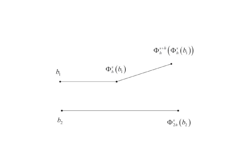
Figure 1:

Triangle inequality gives

$$d(\Phi_{h}^{s+h}\circ\Phi_{h}^{s}(b_{1}),\Phi_{2h}^{s}(b_{2}))\leq d(\Phi_{h}^{s+h}\circ\Phi_{h}^{s}(b_{1}),\Phi_{h}^{s+h}\circ\Phi_{h}^{s}(b_{2}))+d(\Phi_{2h}^{s}(b_{2}),\Phi_{h}^{s+h}\circ\Phi_{h}^{s}(b_{2}))$$ (2.8)

For the first term in the right hand side of (2.8), we use Condition A twice

$$d(\Phi_{h}^{s+h}\circ\Phi_{h}^{s}(b_{1}),\Phi_{h}^{s+h}\circ\Phi_{h}^{s}(b_{2}))\leq d(\Phi_{h}^{s}(b_{1}),\Phi_{h}^{s}(b_{2}))(1+hK_{A})\leq d(b_{1},b_{2})(1+hK_{A})^{2}$$ (2.9)

For the second term, we exploit (2.1) to get

$$d(\Phi_{2h}^{s}(b_{2}),\Phi_{h}^{s+h}\circ\Phi_{h}^{s}(b_{2}))\leq h\tilde{g}(s,h)$$ (2.10)

We combine (2.8), (2.9) and (2.10) to finish the proof. ∎

Remark 2.5.

In general, we have

$$d(\Phi_{h_{2}}^{s+h_{1}}\circ\Phi_{h_{1}}^{s}(b_{1}),\Phi_{h_{1}+h_{2}}^{s}(b_{2}))\leq d(b_{1},b_{2})(1+h_{1}K_{A})(1+h_{2}K_{A})+h_{2}\tilde{g}(h_{1},h_{2})$$ (2.11)

Lemma 2.6.

For a given $a\in X$ and $t\in[0,\infty)$, let $r_{a}$, $\epsilon_{a}$ and $T_{t}$ be the constants in Condition A, B and C. If $b_{1},b_{2}\in B(a,r_{a})$, $h,l+h\in[0,\epsilon_{a}]$, $s,s+l\in[t,T_{t}]$ and $\Phi^{s}_{l}(b_{2})\in B(a,r_{a})$ then we have

$$d(\Phi_{h}^{s+l}(b_{1}),\Phi_{l+h}^{s}(b_{2}))\leq d(b_{1},\Phi_{l}^{s}(b_{2}))+h\eta_{s}(b_{1},b_{2},l,h)$$

where $\eta_{s}(b_{1},b_{2},l,h):=d(b_{1},\Phi_{l}^{s}(b_{2}))K_{A}+\tilde{g}(l,h)$. Furthermore, we notice that $\eta_{s}(b_{1},b_{1},l,h)$ converges to $0$ as $d(b_{1},b_{2}),l,h\rightarrow 0.$

Proof.

We use Condition A and (2.1) to get

$$d(\Phi_{h}^{s+l}(b_{1}),\Phi_{l+h}^{s}(b_{2})) \leq d(\Phi_{h}^{s+l}(b_{1}),\Phi_{h}^{s+l}\circ\Phi_{l}^{s}(b_{2}))+d(\Phi_{h}^{s+l}\circ\Phi_{l}^{s}(b_{2}),\Phi_{l+h}^{s}(b_{2}))$$

$$\leq d(b_{1},\Phi_{l}^{s}(b_{2}))(1+hK_{A})+h\tilde{g}(l,h)$$

$$=d(b_{1},\Phi_{l}^{s}(b_{2}))+h[d(b_{1},\Phi_{l}^{s}(b_{2})K_{A}+\tilde{g}(l,h)]$$

and trivially $\eta_{s}(b_{1},b_{1},l,h)\rightarrow 0$ as $d(b_{1},b_{2}),l,h\rightarrow 0$. ∎

Lemma 2.7.

For a given $a\in X$ and $t\in[0,\infty)$, let $r_{a}$, $\epsilon_{a}$ and $T_{t}$ be the constants in Condition A, B and C. If $b_{1},b_{2}\in B(a,r_{a})$ and $h\in[0,\epsilon_{a}]$, $s,u\in[t,T_{t}]$ then we have,

$$d(\Phi_{h}^{s}(b_{1}),\Phi_{h}^{u}(b_{2}))\leq d(b_{1},b_{2})(1+hK_{A})+Ch|s-u|^{\alpha}$$

Proof.

We combine Condition A and C to get

$$d(\Phi_{h}^{s}(b_{1}),\Phi_{h}^{u}(b_{2})) \leq d(\Phi_{h}^{s}(b_{1}),\Phi_{h}^{s}(b_{2}))+d(\Phi_{h}^{s}(b_{2}),\Phi_{h}^{u}(b_{2}))$$

$$\leq d(b_{1},b_{2})(1+hK_{A})+Ch|s-u|^{\alpha}$$

∎

Lemma 2.8.

For a given $a\in X$ and $t\in[0,\infty)$, let $r_{a}$, $\epsilon_{a}$ and $T_{t}$ be the constants in Condition A, B and C. Assume $b_{1},b_{2}\in B(a,r_{a})$ and $s,s+h\in[t,T_{t}]$. Define a polygonal path $p(l):[0,h]\rightarrow X$ starting at $b_{1}\in X$ as follows; $p(l):=\Phi^{s}_{l}(b_{1})$ for $0\leq l\leq r_{1}$ and $p(l):=\Phi^{s+r_{i}}_{l-r_{i}}(p(r_{i}))$ for $r_{i}\leq l\leq r_{i+1}$ with $0\leq r_{1}\leq\dots\leq r_{i}\leq r_{i+1}\leq\dots\leq r_{k}=h.$ Then we have

$$d(p(l),\Phi_{l}^{s}(b_{2}))\leq d(b_{1},b_{2})+h\max_{1\leq i\leq k}\eta_{s}(p(r_{i}),b_{2},r_{i},r_{i+1}-r_{i})$$ (2.12)

for $0\leq l\leq h$. Furthermore, we have

$$\lim_{h\rightarrow 0}\max_{0\leq r_{i}\leq h}\eta_{s}(p(r_{i}),b_{2},r_{i},r_{i+1}-r_{i})=0$$ (2.13)

Proof.

If $0\leq l\leq r_{1}$ then by Lemma 2.6, we have

$$d(p(l),\Phi_{l}^{s}(b_{2}))\leq d(b_{1},b_{2})+l\eta_{s}(b_{1},b_{2},0,l)$$

For $r_{1}\leq l\leq r_{2}$, we use Lemma 2.6 twice to get

$$d(p(l),\Phi_{l}^{s}(b_{2})) =d(\Phi^{s+r_{1}}_{l-r_{1}}(p(r_{1})),\Phi^{s}_{r_{1}+l-r_{1}}(b_{2}))$$

$$\leq d(p(r_{1}),\Phi_{r_{1}}^{s}(b_{2}))+(l-r_{1})\eta_{s}(p(r_{1}),b_{2},r_{1},l-r_{1})$$

$$\leq d(b_{1},b_{2})+r_{1}\eta_{s}(b_{1},b_{2},0,r_{1})+(l-r_{1})\eta_{s}(p(r_{1}),b_{2},r_{1},l-r_{1})$$

In general, for $r_{i}\leq l\leq r_{i+1}$, we have

$$d(p(l),\Phi_{l}^{s}(b_{2})) \leq d(b_{1},b_{2})+r_{1}\eta_{s}(b_{1},b_{2},0,r_{1})+(r_{2}-r_{1})\eta_{s}(p(r_{1}),b_{2},r_{1},r_{2}-r_{1})$$

$$\qquad\qquad\cdots\quad+(l-r_{i})\eta_{s}(p(r_{i}),b_{2},r_{i},l-r_{i})$$

which gives

$$d(p(l),\Phi_{l}^{s}(b_{2}))\leq d(b_{1},b_{2})+h\max_{1\leq i\leq k}\eta_{s}(p(r_{i}),b_{2},r_{i},r_{i+1}-r_{i})$$

Equation (2.13) is almost trivial since $d(p(r_{i}),b_{2}),r_{i},r_{i+1}-r_{i}$ converge to $0$ as $h\rightarrow 0.$ ∎

2.2 Existence and uniqueness of a solution curve

The proof of the next theorem is similar to the one in [4]. We can also think of it as a corollary of Theorem 3.6. But, to give an idea for the proof of Theorem 3.6 which is more complicated, we give a full proof here.

Theorem 2.9 (Existence).

Let $\Phi:X\times[0,1]\times[0,\infty)$ be an arc field satisfying Condition A, B and C. For a given $a\in X$ and $t\in[0,\infty)$, there exists a solution curve $\sigma:[t,t+c)\rightarrow X$ with initial position $a$ at time $t.$

Proof.

For a positive integer n, we define the n-th discretized solution by

$$\xi_{n}(s):=\left\{\begin{matrix}\Phi_{s}^{t}(a)&0\leq s\leq\frac{1}{2^{n}}\\ \\ \Phi_{s-2^{-n}}^{t+2^{-n}}(\xi_{n}(\frac{1}{2^{n}}))&\frac{1}{2^{n}}\leq s\leq\frac{2}{2^{n}}\\ .\\ .\\ .\\ \Phi_{s-i\cdot 2^{-n}}^{t+i\cdot 2^{-n}}(\xi_{n}(\frac{i}{2^{n}}))&\frac{i}{2^{n}}\leq s\leq\frac{i+1}{2^{n}}\\ .\\ .\end{matrix}\right.$$

Suppose $r,l>0$ are chosen so that $\rho(a,t;r,l)<\infty$. If $\rho(a,t;r,l)=0,$ then $\sigma(s):=a$ defines a solution curve. Thus we assume $\rho(a,t;r,l)>0,$ and let

$$c:=\min\left\{\frac{r}{\rho(a,t;r,l)},l\right\}.$$ (2.14)

It is easy to see that we have $\xi_{n}(s)\in B(a,r)$ for $0\leq s<c$. This implies $\{\xi_{n}\}_{n=1}^{\infty}$ is equi-Lipschitz with Lipschitz constant $\rho(a,t;r,l).$ Moreover, by choosing $r$ smaller if necessary, we may assume that there are constants $K_{A}$, $K_{B}$ and $\epsilon\in(0,1]$ such that $\Lambda(p,q,h)\leq K_{A}$ and $\Omega(p,l^{\prime},h)\leq K_{B}$ for all $p,q\in B(a,r)$ and $l^{\prime},h\in[0,\epsilon]$. We may also assume that $\overline{B(a,r)}$ is a complete metric space.

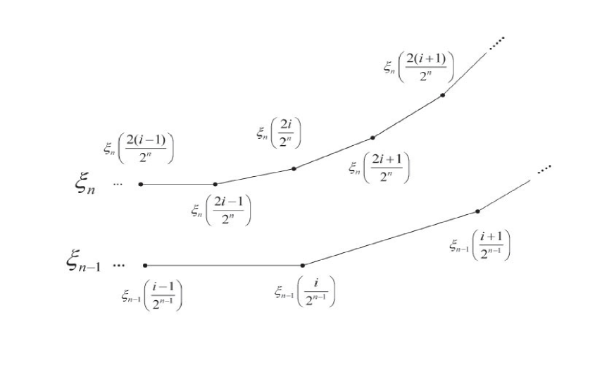
Figure 2:

Let us first estimate the uniform distance between $\xi_{n}$ and $\xi_{n-1}$. We apply Lemma 2.4 with $h=1/2^{n}$ and $b_{1}=b_{2}=a$ to get

$$d\bigl{(}\xi_{n}(\frac{2}{2^{n}}),\xi_{n-1}(\frac{2}{2^{n}})\bigr{)} \leq\frac{1}{2^{n}}\tilde{g}\bigl{(}\frac{1}{2^{n}},\frac{1}{2^{n}}\bigr{)}$$

Similarly, we apply Lemma 2.4 multiple times and get

$$d\bigl{(}\xi_{n}(\frac{2\cdot 2}{2^{n}}),\xi_{n-1}(\frac{2\cdot 2}{2^{n}})\bigr{)} \leq d\bigl{(}\xi_{n}(\frac{2}{2^{n}}),\xi_{n-1}(\frac{2}{2^{n}})\bigr{)}\bigl{(}1+\frac{K_{A}}{2^{n}}\bigr{)}^{2}+\frac{1}{2^{n}}\tilde{g}\bigl{(}\frac{1}{2^{n}},\frac{1}{2^{n}}\bigr{)}$$

$$\leq\frac{1}{2^{n}}\tilde{g}\bigl{(}\frac{1}{2^{n}},\frac{1}{2^{n}}\bigr{)}\bigl{[}1+(1+\frac{K_{A}}{2^{n}})^{2}\bigr{]}$$

$$d\bigl{(}\xi_{n}(\frac{3\cdot 2}{2^{n}}),\xi_{n-1}(\frac{3\cdot 2}{2^{n}})\bigr{)} \leq\frac{1}{2^{n}}\tilde{g}\bigl{(}\frac{1}{2^{n}},\frac{1}{2^{n}}\bigr{)}\bigl{[}1+(1+\frac{K_{A}}{2^{n}})^{2}+(1+\frac{K_{A}}{2^{n}})^{2\cdot 2}\bigr{]}$$

In general, for all i so that $i\cdot 2/2^{-n}\leq c$, we have

$$d\bigl{(}\xi_{n}(\frac{i\cdot 2}{2^{n}}),\xi_{n-1}(\frac{i\cdot 2}{2^{n}})\bigr{)} \leq\frac{1}{2^{n}}\tilde{g}\bigl{(}\frac{1}{2^{n}},\frac{1}{2^{n}}\bigr{)}\sum_{j=0}^{i-1}(1+2^{-n}K_{A})^{2\cdot j}$$

$$=\frac{1}{2^{n}}\tilde{g}\bigl{(}\frac{1}{2^{n}},\frac{1}{2^{n}}\bigr{)}\frac{(1+2^{-n}K_{A})^{2i}-1}{(1+2^{-n}K_{A})^{2}-1}$$

$$\leq\tilde{g}\bigl{(}\frac{1}{2^{n}},\frac{1}{2^{n}}\bigr{)}\frac{(1+2^{-n}K_{A})^{c2^{n}}-1}{K_{A}(2+2^{-n}K_{A})}$$

$$\leq\tilde{g}\bigl{(}\frac{1}{2^{n}},\frac{1}{2^{n}}\bigr{)}\frac{e^{cK_{A}}-1}{K_{A}(2+2^{-n}K_{A})}$$

$$=\tilde{g}\bigl{(}\frac{1}{2^{n}},\frac{1}{2^{n}}\bigr{)}K$$ (2.15)

where $K:=\frac{e^{cK_{A}}-1}{2K_{A}}$ is a constant independent of $n$.

So for any $s\in[0,c)$, let $i$ be an integer such that

$$\frac{2i}{2^{n}}\leq s<\frac{2(i+1)}{2^{n}}$$

then we have

$$d(\xi_{n}(s),\xi_{n-1}(s)) \leq d\bigl{(}\xi_{n}(s),\xi_{n}(\frac{2i}{2^{n}})\bigr{)}+d\bigl{(}\xi_{n}(\frac{2i}{2^{n}}),\xi_{n-1}(\frac{2i}{2^{n}})\bigr{)}+d\bigl{(}\xi_{n-1}(\frac{2i}{2^{n}}),\xi_{n-1}(s)\bigr{)}$$

$$\leq{\rm Lip}(\xi_{n})\bigl{(}s-\frac{2i}{2^{n}}\bigr{)}+\tilde{g}\bigl{(}\frac{1}{2^{n}},\frac{1}{2^{n}}\bigr{)}K+{\rm Lip}(\xi_{n-1})\bigl{(}s-\frac{2i}{2^{n}}\bigr{)}$$

$$\leq\frac{4}{2^{n}}\rho(a,t;r,l)+\tilde{g}\bigl{(}\frac{1}{2^{n}},\frac{1}{2^{n}}\bigr{)}K$$ (2.16)

where we exploit the equi-Lipschitz property of $\xi_{n}$ and (2.2).

Next, we exploit (2.2) to show that $\{\xi_{n}\}$ is a Cauchy sequence in the uniform topology. For any $s\in[0,c)$, we have

$$d(\xi_{n}(s),\xi_{n+m}(s)) \leq\sum_{j=0}^{m-1}d(\xi_{n+j}(s),\xi_{n+j+1}(s))$$

$$\leq\sum_{j=0}^{m-1}\frac{4}{2^{(n+j+1)}}\rho(a,t;r,l)+\tilde{g}\bigl{(}\frac{1}{2^{(n+j+1)}},\frac{1}{2^{(n+j+1)}}\bigr{)}K$$

$$\leq\frac{4}{2^{n+1}}\rho(a,t;r,l)+K\sum_{j=n+1}^{\infty}\tilde{g}(2^{-j},2^{-j})\rightarrow 0\quad{\rm as}\quad n\rightarrow\infty$$ (2.17)

Since $\xi_{n}(s)$ is in the complete space $\overline{B(a,r)},$ we know that $\xi_{n}$ converges uniformly and we define $\tilde{\sigma}:[0,c)\rightarrow X$ by

$$\tilde{\sigma}(s)=\lim_{n\rightarrow\infty}\xi_{n}(s)$$

It is trivial to see $\tilde{\sigma}(0)=a$ and let us check that

$$\lim_{h\rightarrow 0}\frac{d(\tilde{\sigma}(s+h),\Phi_{h}^{t+s}(\tilde{\sigma}(s)))}{h}=0$$ (2.18)

holds for all $s\in[0,c)$. Let $\epsilon>0$ and $h>0$ be fixed such that $s+h<c.$ From triangle inequality, we have

$$\frac{d(\tilde{\sigma}(s+h),\Phi_{h}^{t+s}(\tilde{\sigma}(s)))}{h} \leq\frac{d(\tilde{\sigma}(s+h),\xi_{n}(s+h))}{h}+\frac{d(\xi_{n}(s+h),\Phi_{h}^{t+s}(\xi_{n}(s)))}{h}$$

$$\qquad\qquad\qquad+\frac{d(\Phi_{h}^{t+s}(\xi_{n}(s))\Phi_{h}^{t+s}(\tilde{\sigma}(s)))}{h}$$ (2.19)

Since $\xi_{n}$ converges uniformly, we can choose $n$ large enough so that

$$\frac{d(\tilde{\sigma}(s+h),\xi_{n}(s+h))}{h}+\frac{d(\Phi_{h}^{t+s}(\xi_{n}(s))\Phi_{h}^{t+s}(\tilde{\sigma}(s)))}{h}\leq\frac{\epsilon}{2}$$ (2.20)

We combine (2.2) and (2.20) to get

$$\frac{d(\tilde{\sigma}(s+h),\Phi_{h}^{t+s}(\tilde{\sigma}(s)))}{h}\leq\frac{d(\xi_{n}(s+h),\Phi_{h}^{t+s}(\xi_{n}(s)))}{h}+\frac{\epsilon}{2}$$ (2.21)

We need to estimate the second term of (2.21).

Let $i$ be such that $i/2^{n}\leq s<(i+1)/2^{n},$ then

$$d(\xi_{n}(s+h),\Phi_{h}^{t+s}(\xi_{n}(s))) \leq d\bigl{(}\xi_{n}(s+h),\xi_{n}(\frac{i}{2^{n}}+h)\bigr{)}+d\bigl{(}\xi_{n}(\frac{i}{2^{n}}+h),\Phi_{h}^{t+\frac{i}{2^{n}}}(\xi_{n}(\frac{i}{2^{n}}))\bigr{)}$$

$$\qquad\qquad+d\bigl{(}\Phi_{h}^{t+\frac{i}{2^{n}}}(\xi_{n}(\frac{i}{2^{n}})),\Phi_{h}^{t+s}(\xi_{n}(s))\bigr{)}$$ (2.22)

Let us estimate the righthand side of (2.2) term by term. First, by the Lipschitz property of $\xi_{n}$, we have

$$d\bigl{(}\xi_{n}(s+h),\xi_{n}(\frac{i}{2^{n}}+h)\bigr{)} \leq\bigl{(}s-\frac{i}{2^{n}}\bigr{)}\rho(a,t;r_{a},\epsilon_{a})$$

$$\leq\frac{1}{2^{n}}\rho(a,t;r_{a},\epsilon_{a})$$ (2.23)

For the second term, we use Lemma 2.8 with $\xi_{n}(\frac{i}{2^{n}}):=b_{1}=b_{2}$.

$$d\bigl{(}\xi_{n}(\frac{i}{2^{n}}+h),\Phi_{h}^{t+\frac{i}{2^{n}}}(\xi_{n}(\frac{i}{2^{n}}))\bigr{)}\leq h\sup_{0\leq r\leq h}\eta\bigl{(}\xi_{n}(\frac{i}{2^{n}}+r),\xi_{n}(\frac{i}{2^{n}}),r,\frac{1}{2^{n}}\bigr{)}$$ (2.24)

By using Lemma 2.7 and the Lipschitz property of $\xi_{n}$, we can estimate the last term

$$d\bigl{(}\Phi_{h}^{t+\frac{i}{2^{n}}}(\xi_{n}(t+\frac{i}{2^{n}})),\Phi_{h}^{s}(\xi_{n}(s))\bigr{)} \leq d\bigl{(}\xi_{n}(\frac{i}{2^{n}}),\xi_{n}(s)\bigr{)}(1+hK_{A})+\frac{Ch}{2^{n\alpha}}$$

$$\leq\frac{1}{2^{n}}\rho(a,t;r_{a},\epsilon_{a})(1+hK_{A})+\frac{Ch}{2^{n\alpha}}$$ (2.25)

We combine equations (2.2),(2.2),(2.24) and (2.2), and assume $n$ is large enough to have

$$d(\xi_{n}(s+h),\Phi_{h}^{t+s}(\xi_{n}(s))) \leq h\sup_{0\leq r\leq h}\eta\bigl{(}\xi_{n}(\frac{i}{2^{n}}+r),\xi_{n}(\frac{i}{2^{n}}),r,\frac{1}{2^{n}}\bigr{)}+\frac{1}{2^{n}}\rho(a,t;r_{a},\epsilon_{a})(2+hK_{A})+\frac{Ch}{2^{n\alpha}}$$

$$\leq h\sup_{0\leq r\leq h}\eta\bigl{(}\xi_{n}(\frac{i}{2^{n}}+r),\xi_{n}(\frac{i}{2^{n}}),r,\frac{1}{2^{n}}\bigr{)}+\frac{\epsilon}{2}$$ (2.26)

We combine (2.21) and (2.2), and let $h\rightarrow 0$ with $n$ large

$$\lim_{h\rightarrow 0}\frac{d(\tilde{\sigma}(s+h),\Phi_{h}^{t+s}(\tilde{\sigma}(s)))}{h} \leq\lim_{h\rightarrow 0}\sup_{0\leq r\leq h}\eta\bigl{(}\xi_{n}(\frac{i}{2^{n}}+r),\xi_{n}(\frac{i}{2^{n}}),r,\frac{1}{2^{n}}\bigr{)}+\epsilon$$

$$=\epsilon$$

This gives (2.18). We define $\sigma:[t,t+c)\rightarrow X$ by

$$\sigma(s):=\tilde{\sigma}(s-t),\qquad s\in[t,t+c)$$

It is trivial that $\sigma(t)=\tilde{\sigma}(0)=a$ and (2.18) implies that $\sigma$ satisfies (2.1). This concludes the proof. ∎

Theorem 2.10 (Uniqueness).

Let $\sigma_{a,t}:[t,t+c)\rightarrow X$ be a solution curve of an arc field $\Phi$ with initial position $a$ at time $t$, and let $\sigma_{b,u}:[u,u+c)\rightarrow X$ be a solution curve of $\Phi$ with initial position $b$ at time $u$. Then we have

$$d(\sigma_{a,t}(t+s),\sigma_{b,u}(u+s))\leq e^{K_{A}s}d(a,b)+\tilde{C}|t-u|^{\alpha},\quad{\rm for}\quad s\in[0,c)$$

where $\tilde{C}$ is a constant depending only on $c$ and $K_{A}$.

Proof.

Let us first define $\tilde{\sigma}_{\alpha,\tau}:[0,c)\rightarrow X$ by

$$\tilde{\sigma}_{\alpha,\tau}(s):={\sigma}_{\alpha,\tau}(\tau+s),\qquad{\rm for}\quad s\in[0,c)$$

where $\alpha\in X$ and $\tau\in[0,\infty)$. If we can show

$$d(\tilde{\sigma}_{a,t}(s),\tilde{\sigma}_{b,u}(s))\leq e^{K_{A}s}d(a,b)+\tilde{C}|t-u|^{\alpha},\quad{\rm for}\quad s\in[0,c)$$ (2.27)

for some constant $\tilde{C}$ which is depending only on $c$ and $K_{A}$ then we are done.

Triangle inequality gives

$$d(\tilde{\sigma}_{a,t}(s),\tilde{\sigma}_{b,u}(s))\leq d(\tilde{\sigma}_{a,t}(s),\tilde{\sigma}_{b,t}(s))+d(\tilde{\sigma}_{b,t}(s),\tilde{\sigma}_{b,u}(s))$$ (2.28)

First, let us estimate the second term in the right hand side of (2.28). Let $\xi_{n}^{t}$ be the n-th discretized solution of $\tilde{\sigma}_{b,t}$ and let $\xi_{n}^{u}$ be the n-th discretized solution of $\tilde{\sigma}_{b,u}$. We exploit Condition C and get

$$d_{1}:=d\bigl{(}\xi_{n}^{t}(\frac{1}{2^{n}}),\xi_{n}^{u}(\frac{1}{2^{n}})\bigr{)}\leq\frac{C}{2^{n}}|t-u|^{\alpha}$$ (2.29)

Again, triangle inequality gives

$$d_{2}: =d\bigl{(}\xi_{n}^{t}(\frac{2}{2^{n}}),\xi_{n}^{u}(\frac{2}{2^{n}})\bigr{)}$$

$$\leq d\bigl{(}\xi_{n}^{t}(\frac{2}{2^{n}}),\Phi_{2^{-n}}^{u+2^{-n}}(\xi_{n}^{t}(\frac{1}{2^{n}}))\bigr{)}+d\bigl{(}\Phi_{2^{-n}}^{u+2^{-n}}(\xi_{n}^{t}(\frac{1}{2^{n}})),\xi_{n}^{u}(\frac{2}{2^{n}})\bigr{)}$$

$$=d\bigl{(}\Phi_{2^{-n}}^{t+2^{-n}}(\xi_{n}^{t}(\frac{1}{2^{n}})),\Phi_{2^{-n}}^{u+2^{-n}}(\xi_{n}^{t}(\frac{1}{2^{n}}))\bigr{)}+d\bigl{(}\Phi_{2^{-n}}^{u+2^{-n}}(\xi_{n}^{t}(\frac{1}{2^{n}})),\Phi_{2^{-n}}^{u+2^{-n}}(\xi_{n}^{u}(\frac{1}{2^{n}}))\bigr{)}$$ (2.30)

We exploit Condition C to get

$$d\bigl{(}\Phi_{2^{-n}}^{t+2^{-n}}(\xi_{n}^{t}(\frac{1}{2^{n}})),\Phi_{2^{-n}}^{u+2^{-n}}(\xi_{n}^{t}(\frac{1}{2^{n}}))\bigr{)}\leq\frac{C}{2^{n}}|t-u|^{\alpha}$$ (2.31)

and Condition A gives

$$d\bigl{(}\Phi_{2^{-n}}^{u+2^{-n}}(\xi_{n}^{t}(\frac{1}{2^{n}})),\Phi_{2^{-n}}^{u+2^{-n}}(\xi_{n}^{u}(\frac{1}{2^{n}}))\bigr{)} \leq d\bigl{(}\xi_{n}^{t}(\frac{1}{2^{n}}),\xi_{n}^{u}(\frac{1}{2^{n}})\bigr{)}\bigl{(}1+\frac{K_{A}}{2^{n}}\bigr{)}$$

$$=d_{1}\bigl{(}1+\frac{K_{A}}{2^{n}}\bigr{)}$$ (2.32)

We combine(2.2), (2.31) and (2.2)

$$d_{2} \leq d_{1}\bigl{(}1+\frac{K_{A}}{2^{n}}\bigr{)}+\frac{C}{2^{n}}|t-u|^{\alpha}$$

$$\leq\frac{C}{2^{n}}|t-u|^{\alpha}\bigl{[}1+(1+\frac{K_{A}}{2^{n}})\bigr{]}$$

Similarly, for all $k$ such that $\frac{k}{2^{n}}\leq c$, we have

$$d_{k}: =d\bigl{(}\xi_{n}^{t}(\frac{k}{2^{n}}),\xi_{n}^{u}(\frac{k}{2^{n}})\bigr{)}$$

$$\leq\frac{C}{2^{n}}|t-u|^{\alpha}\bigl{[}1+(1+\frac{K_{A}}{2^{n}})+\cdots+(1+\frac{K_{A}}{2^{n}})^{k-1}\bigr{]}$$

$$\leq\frac{C|t-u|^{\alpha}}{2^{n}}\frac{[1+\frac{K_{A}}{2^{n}}]^{k}-1}{1+\frac{K_{A}}{2^{n}}-1}$$

$$\leq\frac{C(e^{K_{A}/c}-1)}{K_{A}}|t-u|^{\alpha}$$ (2.33)

This means, for all $s$ such that $s<c$

$$d(\xi_{n}^{t}(s),\xi_{n}^{u}(s)\leq\tilde{C}|t-u|^{\alpha}$$ (2.34)

where $\tilde{C}:=C(e^{K_{A}/c}-1)/K_{A}$. Since (2.34) is true for all $n$, we have

$$d(\tilde{\sigma}_{b,t}(s),\tilde{\sigma}_{b,u}(s)\leq\tilde{C}|t-u|^{\alpha}$$ (2.35)

Now, let us estimate the first term in the right hand side of (2.28). We define

$$g(s):=e^{-K_{A}s}d(\tilde{\sigma}_{a,t}(s),\tilde{\sigma}_{b,t}(s))$$

For $h\geq 0$, we have

$$g(s+h)-g(s) =e^{-K_{A}(s+h)}d(\tilde{\sigma}_{a,t}(s+h),\tilde{\sigma}_{b,t}(s+h))-e^{-K_{A}s}d(\tilde{\sigma}_{a,t}(s),\tilde{\sigma}_{b,t}(s))$$

$$\leq e^{-K_{A}(s+h)}(d(\Phi_{h}^{t+s}(\tilde{\sigma}_{a,t}(s)),\Phi_{h}^{t+s}(\tilde{\sigma}_{b,t}(s))+o(h))-e^{-K_{A}s}d(\tilde{\sigma}_{a,t}(s),\tilde{\sigma}_{b,t}(s))$$

$$\leq e^{-K_{A}s}e^{-K_{A}h}d(\tilde{\sigma}_{a,t}(s),\tilde{\sigma}_{b,t}(s))(1+K_{A}h)-e^{-K_{A}s}d(\tilde{\sigma}_{a,t}(s),\tilde{\sigma}_{b,t}(s))+o(h)$$

$$=(e^{-K_{A}h}(1+K_{A}h)-1)e^{-K_{A}s}d(\tilde{\sigma}_{a,t}(s),\tilde{\sigma}_{b,t}(s))+o(h)$$

$$=o(h)(g(s)+1)$$

Hence,

$$D^{+}g(s):={\limsup_{h\rightarrow 0^{+}}}\bigl{(}\frac{g(s+h)-g(s)}{h}\bigr{)}\leq 0$$

Consequently, $g(t)\leq g(0)$ equivalently

$$d(\tilde{\sigma}_{a,t}(s),\tilde{\sigma}_{b,t}(s))\leq e^{K_{A}s}d(a,b),\quad{\rm for}\quad s\in[0,c)$$ (2.36)

(2.35) and (2.36) together with (2.28) give (2.27) and conclude the proof. ∎

2.3 Generating flows

As a corollary of Theorem 2.9 and Theorem 2.10, if an arc field $\Phi$ satisfies Condition A,B and C then there is a unique solution curve $\sigma_{a,t}:[t,t+c_{a,t})\rightarrow X$ with initial position $a$ at time $t,$ for each $a\in X$ and $t\in[0,\infty)$. To guarantee that $c_{a,t}=\infty$ for all $a\in X$ and $t\in[0,\infty)$, we borrow the idea of [4].

Definition 2.11.

An arc field $\Phi$ is said to have linear speed growth if there is a point $x\in X$ positive constants $c_{1}(x)$ and $c_{2}(x)$ such that for all $r>0$ and $t,l>0$

$$\rho(x,t;r,l)\leq c_{1}(x)r+c_{2}(x)$$ (2.37)

Theorem 2.12.

Let $\Phi$ be an arc field which has linear speed growth. Suppose that at each point $a\in X$ and $t\in[0,\infty)$, $\Phi$ has a solution curve $\sigma_{a,t}:[t,t+c_{a,t})\rightarrow X$ with initial position $a$ at time $t$. Then $c_{a,t}$ can be chosen to be $\infty$.

Proof.

Similar to Theorem 4.4 of [4] ∎

3 Adding Flows

3.1 Sum of arc fields

Let $\Phi$ and $\Psi$ be two arc fields satisfying Condition A,B and C. We impose a certain commutation law on $\Phi$ and $\Psi$.
Condition D: There exist constants $0<\alpha<1$ and $C_{d}>0,$ and a function $\Pi:X\times X\times[0,1]\rightarrow R$ such that for each $a\in X$ and $t\in[0,\infty)$, there are constants $r_{a}>0,$ $\epsilon_{a}\in(0,1]$ and $T_{t}>t$ such that $\Pi$ is bounded from above on $B(a,r_{a})\times B(a,r_{a})\times[0,\epsilon_{a}]$ and

$$d(\Phi_{2h}^{s+h}\circ\Psi_{2h}^{s}(b_{1}),\Psi_{2h}^{s+h}\circ\Phi_{2h}^{s}(b_{2}))\leq d(b_{1},b_{2})(1+h\Pi(b_{1},b_{2},h))+C_{d}h^{1+\alpha}$$ (3.1)

for all $b_{1},b_{2}\in B(a,r_{a}),$ $h\in[0,\epsilon_{a}]$ and $s,s+h\in[t,T_{t}]$.

Remark 3.1.

Once we have fixed $a\in X$, $t\in[0,\infty)$ and fixed constants $r_{a},\epsilon_{a},T_{t}$ then the function $\Pi$ is bounded above. We denote upper bound of $\Pi$ by $K_{D}$.

Definition 3.2.

For given $a\in X$ and $t\in[0,\infty),$ a solution curve of the sum of $\Phi$ and $\Psi$ with initial position $a$ at time $t$ is a map $\sigma:[t,t+c)\rightarrow X$ such that $\sigma(t)=a$ and for each $s\in[t,t+c)$

$$\lim_{h\rightarrow 0}\frac{d(\sigma(s+2h),\Psi_{2h}^{s+h}\circ\Phi_{2h}^{s}(\sigma(s)))}{2h}=0$$ (3.2)

Remark 3.3.

If $\Phi$ and $\Psi$ satisfy Condition D, then we can check that

$$\lim_{h\rightarrow 0}\frac{d(\sigma(s+2h),\Psi_{h}^{s+h}\circ\Phi_{h}^{s}(\sigma(s)))}{2h}=\lim_{h\rightarrow 0}\frac{d(\sigma(s+2h),\Phi_{h}^{s+h}\circ\Psi_{h}^{s}(\sigma(s)))}{2h}$$ (3.3)

So, a solution curve of the sum of $\Phi$ and $\Psi$ is a solution curve of the sum of $\Psi$ and $\Phi$.

For a notational convenience in later computations, let us introduce new arc fields $\tilde{\Phi}$ and $\tilde{\Psi}$ which are defined by

$$\tilde{\Phi}_{h}^{s}(b):=\Phi_{2h}^{s}(b),\qquad\tilde{\Psi}_{h}^{s}(b):=\Psi_{2h}^{s}(b)$$

for all $b\in X$ and $(h,s)\in[0,1]\times[0,\infty).$ It is trivial to see if $\Phi$ and $\Psi$ satisfy Condition D then $\tilde{\Phi}$ and $\tilde{\Psi}$ satisfy the following condition
Condition D’: For all $b_{1},b_{2}\in B(a,r_{a}),$ $h\in[0,\epsilon_{a}]$ and $s,s+h\in[t,T_{t}],$ we have

$$d(\tilde{\Phi}_{h}^{s+h}\circ\tilde{\Psi}_{h}^{s}(b_{1}),\tilde{\Psi}_{h}^{s+h}\circ\tilde{\Phi}_{h}^{s}(b_{2}))\leq d(b_{1},b_{2})(1+h{\Pi}(b_{1},b_{2},h))+C_{d}h^{1+\alpha}$$ (3.4)

with same constants $r_{a},$ $\epsilon_{a},$ $T_{t},$ $\alpha,$ $C_{d}$ and a function $\Pi$ as in Condition D.

It is also trivial to see that $\sigma:[t,t+c)\rightarrow X$ is a solution curve of the sum of $\Psi$ and $\Psi$ if and only if $\sigma$ satisfies

$$\lim_{h\rightarrow 0}\frac{d(\sigma(s+2h),\tilde{\Psi}_{h}^{s+h}\circ\tilde{\Phi}_{h}^{s}(\sigma(s)))}{2h}=0$$ (3.5)

for all $s\in[t,t+c).$

Lemma 3.4.

For a given $a\in X$ and $t\in[0,\infty)$, let arc fields $\Phi$ and $\Psi$ satisfy Condition A,B,C and D’, and $r_{a}$, $\epsilon_{a}$ and $T_{t}$ be constants in those conditions. If $b_{1},b_{2}\in B(a,r_{a})$, $4h\in[0,\epsilon_{a}]$ and $s,s+4h\in[t,T_{t}]$ then we have

$$d(\Psi_{h}^{s+3h}\circ\Phi_{h}^{s+2h}\circ\Psi_{h}^{s+h}\circ\Phi_{h}^{s}(b_{1}),\Psi_{2h}^{s+2h}\circ\Phi_{2h}^{s}(b_{2}))\leq d(b_{1},b_{2})(1+hK)^{3}+C(h)$$

where $K:=\max\{K_{A},K_{B},K_{D}\}$ and $C(h):=C_{d}h^{1+\alpha}(1+hK)+h\tilde{g}(h,h)[1+(1+hK)^{2}]$.

Proof.

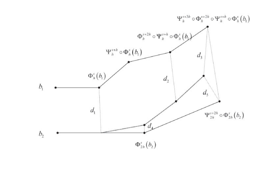
Figure 3:

1. We use Condition A to get,

$$d_{1}:=d(\Phi_{h}^{s}(b_{1}),\Phi_{h}^{s}(b_{2}))\leq d(b_{1},b_{2})(1+hK_{A})$$

2. Condition A and D give,

$$d_{2}: =d(\Phi_{h}^{s+2h}\circ\Psi_{h}^{s+h}(\Phi_{h}^{s}(b_{1})),\Psi_{h}^{s+2h}\circ\Phi_{h}^{s+h}(\Phi_{h}^{s}(b_{2})))$$

$$\leq d(\Phi_{h}^{s}(b_{1}),\Phi_{h}^{s}(b_{2}))(1+hK_{D})+C_{d}h^{1+\alpha}$$

$$\leq d(b_{1},b_{2})(1+hK_{A})(1+hK_{D})+C_{d}h^{1+\alpha}$$ (3.6)

3. We combine Condition A and (3.1) to get

$$d_{3}: =d(\Psi_{h}^{s+3h}(\Phi_{h}^{s+2h}\circ\Psi_{h}^{s+h}\circ\Phi_{h}^{s}(b_{1})),\Psi_{h}^{s+3h}(\Psi_{h}^{s+2h}\circ\Phi_{h}^{s+h}\circ\Phi_{h}^{s}(b_{2})))$$

$$\leq d(\Phi_{h}^{s+2h}\circ\Psi_{h}^{s+h}\circ\Phi_{h}^{s}(b_{1}),\Psi_{h}^{s+2h}\circ\Phi_{h}^{s+h}\circ\Phi_{h}^{s}(b_{2})))(1+hK_{A})$$

$$\leq[d(b_{1},b_{2})(1+hK_{A})(1+hK_{D})+C_{d}h^{1+\alpha}](1+hK_{A})$$ (3.7)

4. Equation (2.1) gives,

$$d_{4}:=d(\Phi_{2h}^{s}(b_{2}),\Phi_{h}^{s+h}\circ\Phi_{h}^{s}(b_{2})))\leq h\tilde{g}(h,h)$$ (3.8)

5. We exploit Lemma 2.4 to have

$$d(\Psi_{h}^{s+3h}\circ\Psi_{h}^{s+2h}(\Phi_{h}^{s+h}\circ\Phi_{h}^{s}(b_{2}))),\Psi_{2h}^{s+2h}(\Phi_{2h}^{s}(b_{2})))\leq d(\Phi_{h}^{s+h}\circ\Phi_{h}^{s}(b_{2})),\Phi_{2h}^{s}(b_{2}))(1+hK_{A})^{2}+h\tilde{g}(h,h)$$

and this together with (3.8) gives

$$d_{5}: =d(\Psi_{h}^{s+3h}\circ\Psi_{h}^{s+2h}(\Phi_{h}^{s+h}\circ\Phi_{h}^{s}(b_{2}))),\Psi_{2h}^{s+2h}(\Phi_{2h}^{s}(b_{2})))$$

$$\leq h\tilde{g}(h,h)(1+hK_{A})^{2}+h\tilde{g}(h,h)$$ (3.9)

Finally, triangle inequality with (3.1) and (3.1) gives

$$d(\Psi_{h}^{s+3h}\circ\Phi_{h}^{s+2h}\circ\Psi_{2h}^{s+h}\circ\Phi_{h}^{s}(b_{1}),\Psi_{2h}^{s+2h}\circ\Phi_{2h}^{s}(b_{2}))$$

$$\leq d_{3}+d_{5}$$

$$\leq d(b_{1},b_{2})(1+hK_{A})^{2}(1+hK_{D})+C_{d}h^{1+\alpha}(1+hK_{A})+h\tilde{g}(h,h)[1+(1+hK_{A})^{2}]$$

∎

Remark 3.5.

By exactly the same argument as in Lemma 3.4, we can show a more general formula: Let $h_{1}:=l_{1}+r$ and $h_{2}:=r+l_{2}$, then we have

$$d(\Psi_{l_{2}}^{s+h_{1}+r}\circ\Phi_{r}^{s+h_{1}}\circ\Psi_{r}^{s+l_{1}}\circ\Phi_{l_{1}}^{s}(b_{1}),\Psi_{h_{2}}^{s+h_{1}}\circ\Phi_{h_{1}}^{s}(b_{2}))$$

$$\qquad\quad\leq d(b_{1},b_{2})(1+l_{1}K_{A})(1+rK_{D})(1+l_{2}K_{A})+C(l_{1},r,l_{2})$$ (3.10)

where $C(l_{1},r,l_{2}):=r\tilde{g}(l_{1},r)(1+l_{2}K_{A})(1+rK_{A})+l_{2}\tilde{g}(r,l_{2})+C_{d}r^{1+\alpha}(1+l_{2}K_{A})$.

If we define $K:=\max\{K_{A},K_{D}\}$ and $u:=\max\{l_{1},r,l_{2}\}$ then (3.5) can be simplified as

$$d(\Psi_{l}^{s+h+r}\circ\Phi_{r}^{s+h}\circ\Psi_{r}^{s+l}\circ\Phi_{l}^{s}(b_{1}),\Psi_{h}^{s+h}\circ\Phi_{h}^{s}(b_{2}))\leq d(b_{1},b_{2})(1+uK)^{3}+C(u)$$ (3.11)

where $C(u):=C_{d}u^{1+\alpha}(1+uK)+u\tilde{g}(u,u)[1+(1+uK)^{2}]$.

3.2 Existence and Uniqueness of a solution for the sum of two arc fields

Theorem 3.6.

(Existence) Let $\Phi,\Psi$ be arc fields satisfying Condition A,B,C and D. Then, for given $a\in X$ and $t\in[0,\infty)$, there is a solution curve $\sigma:[t,t+c)\rightarrow X$ of the sum of $\Phi$ and $\Psi$ with initial position $a$ at time $t.$

Proof.

Without loss of generality, we assume $\Phi$ and $\Psi$ satisfy Condition A,B,C and D’, and find a curve $\sigma$ satisfying (3.5).

For a positive integer n, we define the n-th discretized solution by

$$\xi_{n}(s):=\left\{\begin{matrix}\Phi_{s}^{t}(a)&0\leq s\leq\frac{1}{2^{n}}\\ \\ \Psi_{s-2^{-n}}^{t+2^{-n}}(\xi_{n}(\frac{1}{2^{n}}))&\frac{1}{2^{n}}\leq s\leq\frac{2}{2^{n}}\\ .\\ .\\ .\\ \Phi_{s-i\cdot 2^{-n}}^{t+i\cdot 2^{-n}}(\xi_{n}(\frac{i}{2^{n}}))&\frac{i}{2^{n}}\leq s\leq\frac{i+1}{2^{n}}\quad{\rm if}\quad i=2m\\ \\ \Psi_{s-i\cdot 2^{-n}}^{t+i\cdot 2^{-n}}(\xi_{n}(\frac{i}{2^{n}}))&\frac{i}{2^{n}}\leq s\leq\frac{i+1}{2^{n}}\quad{\rm if}\quad i=2m+1\\ .\\ .\end{matrix}\right.$$

Suppose $r,l>0$ are chosen so that $\rho(a,t;r,l)<\infty$. If $\rho(a,t;r,l)=0,$ then $\sigma(s):=a$ defines a solution curve. Thus we assume $\rho(a,t;r,l)>0,$ and let

$$c:=\min\left\{\frac{r}{\rho(a,t;r,l)},l\right\}$$ (3.12)

It is easy to see that we have $\xi_{n}(s)\in B(a,r)$ for $0\leq s<c$. This also implies $\{\xi_{n}\}_{n=1}^{\infty}$ is equi-Lipschitz with Lipschitz constant $\rho(a,t;r,l).$ Moreover, by choosing $r$ smaller if necessary, we may assume there are constants $K_{A}$, $K_{B}$ and $\epsilon\in(0,1]$ such that $\Lambda(p,q,h)\leq K_{A}$ and $\Omega(p,l^{\prime},h)\leq K_{B}$ for all $p,q\in B(a,r)$ and $l,h^{\prime}\in[0,\epsilon]$. We may also assume $\overline{B(a,r)}$ is a complete metric space.

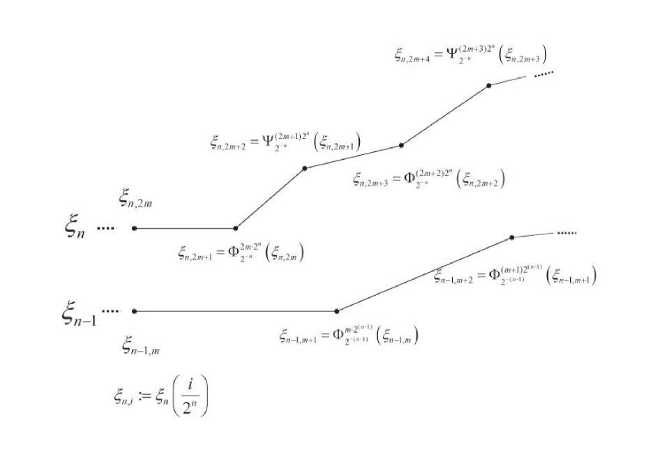
Figure 4:

Let us first estimate the uniform distance between $\xi_{n}$ and $\xi_{n-1}$. We apply Lemma 3.4 with $h:=1/2^{n}$, $s:=t+\frac{4i}{2^{n}}$, $b_{1}:=\xi_{n}(\frac{4i}{2^{n}})$ and $b_{2}:=\xi_{n-1}(\frac{4i}{2^{n}})$ to have

$$d\bigl{(}\xi_{n}\bigl{(}\frac{4(i+1)}{2^{n}}\bigr{)},\xi_{n-1}\bigl{(}\frac{4(i+1)}{2^{n}}\bigr{)}\bigr{)} =d\bigl{(}\Psi_{h}^{s+3h}\circ\Phi_{h}^{s+2h}\circ\Psi_{h}^{s+h}\circ\Phi_{h}^{s}(\xi_{n}(\frac{4i}{2^{n}})),\Psi_{2h}^{s+2h}\circ\Phi_{2h}^{s}(\xi_{n-1}(\frac{4i}{2^{n}}))\bigr{)}$$

$$\leq d\bigl{(}\xi_{n}(\frac{4i}{2^{n}}),\xi_{n-1}(\frac{4i}{2^{n}})\bigr{)}\bigl{(}1+\frac{K}{2^{n}}\bigr{)}^{3}+C\bigl{(}\frac{1}{2^{n}}\bigr{)}$$

where $K:=\max\{K_{A},K_{D}\}$ and $C(h)=C_{d}h^{1+\alpha}(1+hK)+h\tilde{g}(h,h)[1+(1+hK)^{2}]$.

In general, we have

$$d\bigl{(}\xi_{n}(\frac{4(i+1)}{2^{n}}),\xi_{n-1}(\frac{4(i+1)}{2^{n}})\bigr{)} \leq d\bigl{(}\xi_{n}(\frac{4i}{2^{n}}),\xi_{n-1}(\frac{4i}{2^{n}})\bigr{)}\bigl{(}1+\frac{K}{2^{n}}\bigr{)}^{3}+C\bigl{(}\frac{1}{2^{n}}\bigr{)}$$

$$\leq d\bigl{(}\xi_{n}(\frac{4(i-1)}{2^{n}}),\xi_{n-1}(\frac{4(i-1)}{2^{n}})\bigr{)}\bigl{(}1+\frac{K}{2^{n}}\bigr{)}^{3\cdot 2}+C\bigl{(}\frac{1}{2^{n}}\bigr{)}\bigl{[}1+(1+\frac{K}{2^{n}})^{3}\bigr{]}$$

$$...$$

$$\leq d(\xi_{n}(0),\xi_{n-1}(0))\bigl{(}1+\frac{K}{2^{n}}\bigr{)}^{3(i+1)}+C\bigl{(}\frac{1}{2^{n}}\bigr{)}\bigl{[}1+\bigl{(}1+\frac{K}{2^{n}}\bigr{)}^{3}+\cdots+\bigl{(}1+\frac{K}{2^{n}}\bigr{)}^{3i}\bigr{]}$$

Since $\xi_{n}(0)=\xi_{n-1}(0)$, for all $i$ such that $4(i+1)/2^{n}\leq c$, we have

$$d\bigl{(}\xi_{n}(\frac{4(i+1)}{2^{n}}),\xi_{n-1}(\frac{4(i+1)}{2^{n}})\bigr{)} \leq C(2^{-n})\frac{(1+2^{-n}K)^{3i}-1}{(1+2^{-n}K)^{3}-1}$$

$$\leq C(2^{-n})\frac{e^{\frac{3c}{4}K}-1}{2^{-n}K[(1+2^{-n}K)^{2}+(1+2^{-n}K)+1]}$$

$$\leq\frac{C(2^{-n})}{2^{-n}}\frac{e^{\frac{3c}{4}K}-1}{3K}$$ (3.13)

Notice, for sufficiently small $h$

$$C(h)=C_{d}h^{1+\alpha}(1+hK)+h\tilde{g}(h,h)[1+(1+hK)^{2}]\leq 3h[C_{d}h^{\alpha}+\tilde{g}(h,h)]$$ (3.14)

We assume $n$ is large enough in (3.2). We combine that with (3.14) to show

$$d\bigl{(}\xi_{n}(\frac{4(i+1)}{2^{n}}),\xi_{n-1}(\frac{4(i+1)}{2^{n}})\bigr{)}\leq\bigl{[}C_{d}(\frac{1}{2^{n}})^{\alpha}+\tilde{g}(\frac{1}{2^{n}},\frac{1}{2^{n}})\bigr{]}A$$ (3.15)

where $A:=\frac{e^{\frac{3c}{4}K}-1}{K}$. We notice $A$ is independent of $n$.

So for any $s\in[0,c)$, let $i$ be an integer such that

$$\frac{4i}{2^{n}}\leq s<\frac{4(i+1)}{2^{n}}$$

then we have

$$d(\xi_{n}(s),\xi_{n-1}(s)) \leq d\bigl{(}\xi_{n}(s),\xi_{n}(\frac{4i}{2^{n}})\bigr{)}+d\bigl{(}\xi_{n}(\frac{4i}{2^{n}}),\xi_{n-1}(\frac{4i}{2^{n}})\bigr{)}+d\bigl{(}\xi_{n-1}(\frac{4i}{2^{n}}),\xi_{n-1}(s)\bigr{)}$$

$$\leq\frac{8}{2^{n}}\rho(a,t;r,l)+\bigl{[}C_{d}\bigl{(}\frac{1}{2^{n}}\bigr{)}^{\alpha}+\tilde{g}\bigl{(}\frac{1}{2^{n}},\frac{1}{2^{n}}\bigr{)}\bigr{]}A$$ (3.16)

where we use the equi-Lipschitz property of $\xi_{n}$ and (3.15).

Next we exploit (3.2) to show $\xi_{n}$ is a Cauchy sequence in the uniform topology. For any $s\in[0,c)$, we have

$$d(\xi_{n}(s),\xi_{n+m}(s)) \leq\sum_{j=0}^{m-1}d(\xi_{n+j}(s),\xi_{n+j+1}(s))$$

$$\leq\sum_{j=0}^{m-1}\bigl{[}\frac{8}{2^{n+j+1}}\rho(a,t;r,l)+\{C_{d}\bigl{(}\frac{1}{2^{n+j+1}}\bigr{)}^{\alpha}+\tilde{g}\bigl{(}\frac{1}{2^{n+j+1}},\frac{1}{2^{n+j+1}}\bigr{)}\}A\bigr{]}$$

$$\leq\frac{8}{2^{n+1}}\rho(a,t;r,l)+A\sum_{j=n+1}^{\infty}\bigl{[}C_{d}\bigl{(}\frac{1}{2^{n+j+1}}\bigr{)}^{\alpha}+\tilde{g}\bigl{(}\frac{1}{2^{n+j+1}},\frac{1}{2^{n+j+1}}\bigr{)}\bigr{]}$$

$$\rightarrow 0\quad{\rm as}\quad n\rightarrow 0$$

Since $\xi_{n}(s)$ is in the complete space $\overline{B(a,r)}$, we know that $\xi_{n}$ converges uniformly. We define $\tilde{\sigma}:[0,c)\rightarrow X$ by the limit i.e

$$\tilde{\sigma}(s)=\lim_{n\rightarrow\infty}\xi_{n}(s)$$

Next, we are going to show that

$$\lim_{h\rightarrow 0}\frac{d(\tilde{\sigma}(s+2h),\Psi_{h}^{t+s+h}\circ\Phi_{h}^{t+s}(\tilde{\sigma}(s)))}{2h}=0$$ (3.17)

for all $s\in[0,c)$. Once we have (3.17), we are done with the proof by defining a solution curve $\sigma:[t,t+c)\rightarrow X$ as

$$\sigma(s):=\tilde{\sigma}(s-t),\qquad{\rm for}\quad s\in[t,t+c)$$

To prove (3.17), we choose an arbitrary $s\in[0,c)$. Let $\epsilon>0$ and $h>0$ be fixed such that $s+h<c$. From triangle inequality, we have

$$\frac{d(\tilde{\sigma}(s+2h),\Psi_{h}^{t+s+h}\circ\Phi_{h}^{t+s}(\tilde{\sigma}(s)))}{h} \leq\frac{d(\tilde{\sigma}(s+2h),\xi_{n}(s+2h))}{h}+\frac{d(\xi_{n}(s+2h),\Psi_{h}^{t+s+h}\circ\Phi_{h}^{t+s}(\xi_{n}(s)))}{h}$$

$$\qquad+\frac{d(\Psi_{h}^{t+s+h}\circ\Phi_{h}^{t+s}(\xi_{n}(s)),\Psi_{h}^{t+s+h}\circ\Phi_{h}^{t+s}(\tilde{\sigma}(s)))}{h}$$ (3.18)

Since $\xi_{n}$ converges uniformly, we can choose $n$ large enough so that

$$\frac{d(\tilde{\sigma}(s+2h),\xi_{n}(s+2h))}{h}+\frac{d(\Psi_{h}^{t+s+h}\circ\Phi_{h}^{t+s}(\xi_{n}(s)),\Psi_{h}^{t+s+h}\circ\Phi_{h}^{t+s}(\tilde{\sigma}(s)))}{h}\leq\frac{\epsilon}{2}$$ (3.19)

We combine (3.2) and (3.19) to get

$$\frac{d(\tilde{\sigma}(s+2h),\Psi_{h}^{t+s+h}\circ\Phi_{h}^{t+s}(\tilde{\sigma}(s)))}{h}\leq\frac{d(\xi_{n}(s+2h),\Psi_{h}^{t+s+h}\circ\Phi_{h}^{t+s}(\xi_{n}(s)))}{h}+\frac{\epsilon}{2}$$ (3.20)

We need to estimate the second term of (3.20).

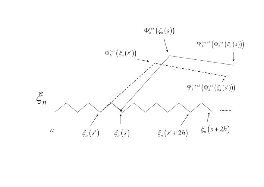
Figure 5:

Let $l$ be a nonnegative integer such that

$$\frac{2l}{2^{n}}\leq s<\frac{2(l+1)}{2^{n}}$$

and define $s^{\prime}:=\frac{2l}{2^{n}}$, then

$$d(\xi_{n}(s+2h),\Psi_{h}^{t+s+h}\circ\Phi_{h}^{t+s}(\xi_{n}(s))) \leq d(\xi_{n}(s+2h),\xi_{n}(s^{\prime}+2h))+d(\xi_{n}(s^{\prime}+2h),\Psi_{h}^{t+s^{\prime}+h}\circ\Phi_{h}^{t+s^{\prime}}(\xi_{n}(s^{\prime})))$$

$$\qquad+d(\Psi_{h}^{t+s^{\prime}+h}\circ\Phi_{h}^{t+s^{\prime}}(\xi_{n}(s^{\prime})),\Psi_{h}^{t+s^{\prime}+h}\circ\Phi_{h}^{t+s^{\prime}}(\xi_{n}(s)))$$

$$\qquad+d(\Psi_{h}^{t+s^{\prime}+h}\circ\Phi_{h}^{t+s^{\prime}}(\xi_{n}(s)),\Psi_{h}^{t+s^{\prime}+h}\circ\Phi_{h}^{t+s}(\xi_{n}(s)))$$

$$\qquad+d(\Psi_{h}^{t+s^{\prime}+h}\circ\Phi_{h}^{t+s}(\xi_{n}(s)),\Psi_{h}^{t+s+h}\circ\Phi_{h}^{t+s}(\xi_{n}(s)))$$

$$\leq d(\xi_{n}(s^{\prime}+2h),\Psi_{h}^{t+s^{\prime}+h}\circ\Phi_{h}^{t+s^{\prime}}(\xi_{n}(s^{\prime})))$$

$$\qquad+\rho(a,t;r,l)(s-s^{\prime})[1+(1+hK_{A})^{2}]$$

$$\qquad+Ch(s-s^{\prime})^{\alpha}[1+(1+hK_{A})]$$ (3.21)

where we use Condition C and the Lipschitz continuity of $\xi_{n}$ in the second inequality. For $n$ large enough, $s-s^{\prime}$ is sufficiently small so that

$$\frac{\rho(a,t;r,l)(s-s^{\prime})[1+(1+hK_{A})^{2}]+Ch(s-s^{\prime})^{\alpha}[1+(1+hK_{A})]}{h}\leq\frac{\epsilon}{2}$$ (3.22)

We combine (3.2) and (3.22) to get

$$\frac{d(\xi_{n}(s+2h),\Psi_{h}^{t+s+h}\circ\Phi_{h}^{t+s}(\xi_{n}(s)))}{h} \leq\frac{d(\xi_{n}(s^{\prime}+2h),\Psi_{h}^{t+s^{\prime}+h}\circ\Phi_{h}^{t+s^{\prime}}(\xi_{n}(s^{\prime})))}{h}+\frac{\epsilon}{2}$$ (3.23)

We need to estimate the second term of (3.23). For the moment, let us assume $h=1/2^{j}$ for some $j\in N$ . With this assumption, we can apply Lemma 3.8 with $m:=n-j$ and $b:=\xi_{n}(s^{\prime})$, and get

$$d(\Psi_{h}^{t+s^{\prime}+h}\circ\Phi_{h}^{t+s^{\prime}}(\xi_{n}(s^{\prime})),\xi_{n}(s^{\prime}+2h)) \leq Ch\bigl{[}h^{\alpha}+\sum_{i=1}^{n-j}\tilde{g}\bigl{(}\frac{h}{2^{i}},\frac{h}{2^{i}}\bigr{)}\bigr{]}$$

$$=\frac{C}{2^{j}}\bigl{[}\bigl{(}\frac{1}{2^{j}}\bigr{)}^{\alpha}+\sum_{i=1}^{n-j}\tilde{g}\bigl{(}\frac{1}{2^{i+j}},\frac{1}{2^{i+j}}\bigr{)}\bigr{]}$$

$$\leq\frac{C}{2^{j}}\bigl{[}\bigl{(}\frac{1}{2^{j}}\bigr{)}^{\alpha}+\sum_{i=j+1}^{\infty}\tilde{g}\bigl{(}\frac{1}{2^{i}},\frac{1}{2^{i}}\bigr{)}\bigr{]}$$ (3.24)

Notice (3.2) is independent of $n$, i.e it holds uniformly for large $n\in N$. Now we combine (3.2), (3.23) and (3.2), and let $h(=1/2^{j})\rightarrow 0$ then

$$\lim_{h\rightarrow 0}\frac{d(\tilde{\sigma}(t+2h),\Psi_{h}^{t+h}\circ\Phi_{h}^{t}(\tilde{\sigma}(t)))}{h} \leq\lim_{j\rightarrow\infty}C\bigl{[}\bigl{(}{\frac{1}{2^{j}}}\bigr{)}^{\alpha}+\sum_{i=j+1}^{\infty}\tilde{g}\bigl{(}\frac{1}{2^{i}},\frac{1}{2^{i}}\bigr{)}\bigr{]}+\epsilon=\epsilon$$ (3.25)

This gives (3.17).

For general $h$, let $k$ be an integer satisfying

$$\frac{k}{2^{n}}\leq h<\frac{k+1}{2^{n}}$$ (3.26)

and define $h^{\prime}:=\frac{k}{2^{n}}$. We exploit Lemma 3.7 to estimate the last term in (3.20) and get

$$\frac{d(\xi_{n}(s+2h),\Psi_{h}^{t+s+h}\circ\Phi_{h}^{t+s}(\xi_{n}(s)))}{h}\leq \frac{d(\xi_{n}(s+2h^{\prime}),\Psi_{h^{\prime}}^{t+s+h^{\prime}}\circ\Phi_{h^{\prime}}^{t+s}(\xi_{n}(s)))}{h^{\prime}}$$

$$+C\bigl{[}\frac{1}{k}+(\frac{1}{2^{n}})^{\alpha}\bigr{]}$$

$$\leq \frac{d(\xi_{n}(s+2h^{\prime}),\Psi_{h^{\prime}}^{t+s+h^{\prime}}\circ\Phi_{h^{\prime}}^{t+s}(\xi_{n}(s)))}{h^{\prime}}+\frac{\epsilon}{2}$$ (3.27)

where we assumed $n$ is large enough to get second inequality. We combine (3.20) and (3.2)

$$\frac{d(\tilde{\sigma}(s+2h),\Psi_{h}^{t+s+h}\circ\Phi_{h}^{t+s}(\tilde{\sigma}(s)))}{h}\leq\frac{d(\Psi_{h^{\prime}}^{t+s+h^{\prime}}\circ\Phi_{h^{\prime}}^{t+s}(\xi_{n}(s)),\xi_{n}(s+2h^{\prime}))}{h^{\prime}}+\epsilon$$ (3.28)

Let $m$ be a nonnegative integer such that $2^{m}\leq k<2^{m+1}$ i.e

$$\frac{2^{m}}{2^{n}}\leq h^{\prime}<\frac{2^{m+1}}{2^{n}}$$ (3.29)

From Remark 3.9 with $b:=\xi_{n}(s)$ and $u:=h^{\prime}/k$, we have

$$d(\Psi_{h^{\prime}}^{t+s+h^{\prime}}\circ\Phi_{h^{\prime}}^{t+s}(\xi_{n}(s)),\xi_{n}(s+2h^{\prime}))\leq C2h^{\prime}\bigl{[}(2h^{\prime})^{\alpha}+\sum_{i=m+2}^{\infty}\tilde{g}\bigl{(}\frac{1}{2^{i}},\frac{1}{2^{i}}\bigr{)}\bigr{]}$$ (3.30)

We combine (3.28) and (3.30) to get

$$\frac{d(\tilde{\sigma}(s+2h),\Psi_{h}^{t+s+h}\circ\Phi_{h}^{t+s}(\tilde{\sigma}(s)))}{h}\leq 2C\bigl{[}(2h^{\prime})^{\alpha}+\sum_{i=m+2}^{\infty}\tilde{g}\bigl{(}\frac{1}{2^{i}},\frac{1}{2^{i}}\bigr{)}\bigr{]}+\epsilon$$ (3.31)

Notice that $h^{\prime}$ converges to $h$ and $m$ increase to $\infty$ as $n\rightarrow\infty$. This implies, for all sufficiently large $n$, we have

$$2C\bigl{[}(2h^{\prime})^{\alpha}+\sum_{i=m+2}^{\infty}\tilde{g}\bigl{(}\frac{1}{2^{i}},\frac{1}{2^{i}}\bigr{)}\bigr{]}\leq 2C(2h)^{\alpha}+\epsilon$$ (3.32)

which is independent of $n$. We combine (3.31) and (3.32), and let $h$ converge to $0$ then we have

$$\lim_{h\rightarrow 0}\frac{d(\tilde{\sigma}(s+2h),\Psi_{h}^{t+s+h}\circ\Phi_{h}^{t+s}(\tilde{\sigma}(s)))}{h}\leq\lim_{h\rightarrow 0}2C(2h)^{\alpha}+\epsilon=\epsilon$$

This gives (3.17) and concludes the proof. ∎

Lemma 3.7.

Let $\xi_{n}:[0,c)\rightarrow X$ be the n-th discretized solution constructed in Theorem 3.6 and $0<h<c$ be fixed. If $k/2^{n}\leq h<(k+1)/2^{n}$ for some integer $k$ then there is a constant $C>0$ such that

$$\frac{d(\Psi_{h}^{u+h}\circ\Phi_{h}^{u}(\xi_{n}(s)),\xi_{n}(s+2h))}{h} \leq\frac{d(\Psi_{h^{\prime}}^{u+h^{\prime}}\circ\Phi_{h^{\prime}}^{u}(\xi_{n}(s)),\xi_{n}(s+2h^{\prime}))}{h}+C\frac{|h-h^{\prime}|}{h}$$

$$\qquad\qquad\qquad+C|h-h^{\prime}|^{\alpha}$$

Here, $h^{\prime}=k/2^{n}$ and $C$ depends only on $c$ and $K_{A}.$

Proof.

Triangle inequality gives

$$d(\Psi_{h}^{u+h}\circ\Phi_{h}^{u}(\xi_{n}(s)),\xi_{n}(s+2h))$$

$$\leq d(\Psi_{h}^{u+h}\circ\Phi_{h}^{u}(\xi_{n}(s)),\Psi_{h^{\prime}}^{u+h^{\prime}}\circ\Phi_{h^{\prime}}^{u}(\xi_{n}(s)))+d(\Psi_{h^{\prime}}^{u+h^{\prime}}\circ\Phi_{h^{\prime}}^{u}(\xi_{n}(s)),\xi_{n}(s+2h^{\prime}))$$

$$\quad+d(\xi_{n}(s+2h^{\prime}),\xi_{n}(s+2h))$$ (3.33)

Let us first estimate the last term of (3.2)

$$d(\xi_{n}(s+2h^{\prime}),\xi_{n}(s+2h))\leq 2\rho(a,t;r,l)|h-h^{\prime}|$$ (3.34)

which comes from the Lipschitz continuity of $\xi_{n}$.

To estimate the first term of (3.2), we exploit triangle inequality

$$d(\Psi_{h}^{u+h}\circ\Phi_{h}^{u}(\xi_{n}(s)),\Psi_{h^{\prime}}^{u+h^{\prime}}\circ\Phi_{h^{\prime}}^{u}(\xi_{n}(s))) \leq d(\Psi_{h}^{u+h^{\prime}}\circ\Phi_{h}^{u}(\xi_{n}(s)),\Psi_{h^{\prime}}^{u+h^{\prime}}\circ\Phi_{h^{\prime}}^{u}(\xi_{n}(s)))$$

$$\qquad+d(\Psi_{h}^{u+h}\circ\Phi_{h}^{u}(\xi_{n}(s)),\Psi_{h}^{u+h^{\prime}}\circ\Phi_{h}^{u}(\xi_{n}(s)))$$ (3.35)

Let us estimate the righthand side of (3.2) term by term. For the first term, we use the Lipschitz continuity of $\Phi,\Psi$ and Condition A to get

$$d(\Psi_{h}^{u+h^{\prime}}\circ\Phi_{h}^{u}(\xi_{n}(s)),\Psi_{h^{\prime}}^{u+h^{\prime}}\circ\Phi_{h^{\prime}}^{u}(\xi_{n}(s))) \leq d(\Psi_{h}^{u+h^{\prime}}\circ\Phi_{h}^{u}(\xi_{n}(s)),\Psi_{h^{\prime}}^{u+h^{\prime}}\circ\Phi_{h}^{u}(\xi_{n}(s)))$$

$$\qquad\qquad+d(\Psi_{h^{\prime}}^{u+h^{\prime}}\circ\Phi_{h}^{u}(\xi_{n}(s)),\Psi_{h^{\prime}}^{u+h^{\prime}}\circ\Phi_{h^{\prime}}^{u}(\xi_{n}(s)))$$

$$\leq\rho(a,t;r,l)|h-h^{\prime}|$$

$$\qquad\qquad+d(\Phi_{h}^{u}(\xi_{n}(s)),\Phi_{h^{\prime}}^{u}(\xi_{n}(s)))(1+hK_{A})$$

$$\leq\rho(a,t;r,l)|h-h^{\prime}|[1+(1+hK_{A})]$$ (3.36)

For the second term, we use Condition C and get

$$d(\Psi_{h}^{u+h}\circ\Phi_{h}^{u}(\xi_{n}(s)),\Psi_{h}^{u+h^{\prime}}\circ\Phi_{h}^{u}(\xi_{n}(s)))\leq Ch|h-h^{\prime}|^{\alpha}$$ (3.37)

Combine (3.2),(3.2) and (3.37)

$$d(\Psi_{h}^{u+h}\circ\Phi_{h}^{u}(\xi_{n}(s)),\Psi_{h^{\prime}}^{u+h^{\prime}}\circ\Phi_{h^{\prime}}^{u}(\xi_{n}(s))) \leq\rho(a,t;r,l)|h-h^{\prime}|[1+(1+hK_{A})]$$

$$\qquad+Ch|h-h^{\prime}|^{\alpha}$$ (3.38)

Finally, (3.2), (3.34) and (3.2) give

$$d(\Psi_{h}^{u+h}\circ\Phi_{h}^{u}(\xi_{n}(s)),\xi_{n}(s+2h)) \leq d(\Psi_{h^{\prime}}^{u+h^{\prime}}\circ\Phi_{h^{\prime}}^{u}(\xi_{n}(s)),\xi_{n}(s+2h^{\prime}))$$

$$\quad+\rho(a,t;r,l)|h-h^{\prime}|[3+(1+hK_{A})]+Ch|h-h^{\prime}|^{\alpha}$$ (3.39)

Which concludes the proof.

∎

Lemma 3.8.

Let $\Phi$ and $\Psi$ be arc fields satisfying Condition A,B,C and D’. For given $a\in X$ and $t\in[0,\infty)$, let $r_{a},\epsilon_{a}$ and $T_{t}$ be constants in those conditions. For $b\in B(a,r_{a})$, $h\in[0,\epsilon_{a}]$ and $s,s+h\in[t,T_{t}],$ there exists a constant $C>0$ such that

$$d(\Psi_{h}^{s+h}\circ\Phi_{h}^{s}(b),\Psi_{h/2^{n}}^{s+(2^{m+1}-1)h/2^{n}}\circ\Phi_{h/2^{n}}^{s+(2^{m+1}-2)h/2^{n}}\circ\cdots\circ\Psi_{h/2^{n}}^{s+h/2^{n}}\circ\Phi_{h/2^{n}}^{s}(b))\leq Ch\bigl{[}h^{\alpha}+\sum_{i=1}^{m}\tilde{g}\bigl{(}\frac{h}{2^{i}},\frac{h}{2^{i}}\bigr{)}\bigr{]}$$

where $m$ and $n$ are nonnegative integers satisfying $m\leq n.$ Here, $C$ depends only on $K$ and $T_{t}.$

Proof.

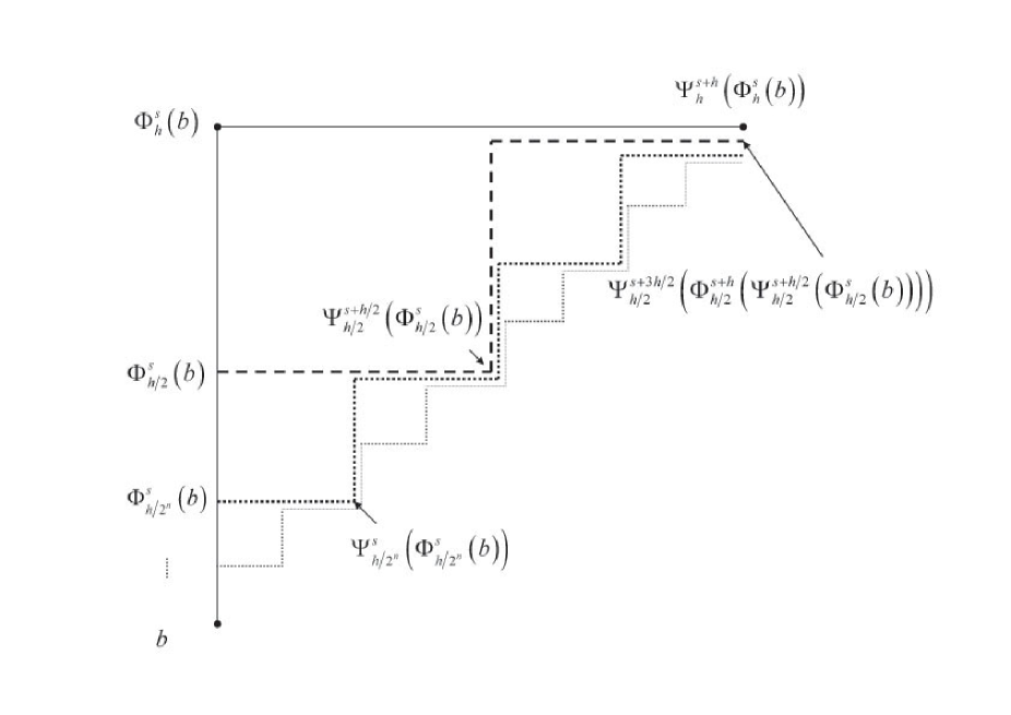
Figure 6:

We use Lemma 3.4,

$$d_{1}:=d(\Psi_{h}^{s+h}\circ\Phi_{h}^{s}(b),\Psi_{h/2}^{s+3h/2}\circ\Phi_{h/2}^{s+h}\circ\Psi_{h/2}^{s+h/2}\circ\Phi_{h/2}^{s}(b))\leq C\bigl{(}\frac{h}{2}\bigr{)}$$

where $C(h):=C_{d}h^{1+\alpha}(1+hK)+h\tilde{g}(h,h)[1+(1+hK)^{2}]$.

$$d_{2}: =d(\Psi_{h/2}^{s+3h/2}\circ\Phi_{h/2}^{s+h}\circ\Psi_{h/2}^{s+h/2}\circ\Phi_{h/2}^{s}(b),\Psi_{h/2^{2}}^{s+7h/2^{2}}\circ\Phi_{h/2^{2}}^{s+6h/2^{2}}\circ\cdots\circ\Psi_{h/2^{2}}^{s+h/2^{2}}\circ\Phi_{h/2^{2}}^{s}(b))$$

$$\leq\tilde{d}_{2}\bigl{(}1+\frac{h}{2^{2}}K\bigr{)}^{3}+C\bigl{(}\frac{h}{2^{2}}\bigr{)}$$ (3.40)

where $\tilde{d}_{2}:=d(\Psi_{h/2}^{s+h/2}\circ\Phi_{h/2}^{s}(b),\Psi_{h/2^{2}}^{s+3h/2^{2}}\circ\Phi_{h/2^{2}}^{s+2h/2^{2}}\circ\Psi_{h/2^{2}}^{s+h/2^{2}}\circ\Phi_{h/2^{2}}^{s}(b))$.

Again, by Lemma 3.4

$$\tilde{d}_{2}\leq C\bigl{(}\frac{h}{2^{2}}\bigr{)}$$ (3.41)

We combine (3.2) and (3.41) to get

$$d_{2}\leq C\bigl{(}\frac{h}{2^{2}}\bigr{)}\bigl{[}1+\bigl{(}1+\frac{h}{2^{2}}K\bigr{)}^{3}\bigr{]}$$ (3.42)

Similarly,

$$d_{3}: =d(\Psi_{h/2^{2}}^{s+7h/2^{2}}\circ\Phi_{h/2^{2}}^{s+6h/2^{2}}\circ\cdots\circ\Psi_{h/2^{2}}^{s+h/2^{2}}\circ\Phi_{h/2^{2}}^{s}(b),\Psi_{h/2^{3}}^{s+15h/2^{3}}\circ\Phi_{h/2^{3}}^{s+14h/2^{3}}\circ\cdots\circ\Psi_{h/2^{3}}^{s+h/2^{3}}\circ\Phi_{h/2^{3}}^{s}(b))$$

$$\leq C\bigl{(}\frac{h}{2^{3}}\bigr{)}\bigl{[}1+(1+\frac{h}{2^{3}}K)^{3}+\bigl{(}1+\frac{h}{2^{3}}K\bigr{)}^{2\cdot 3}+\bigl{(}1+\frac{h}{2^{3}}K\bigr{)}^{3\cdot 3}\bigr{]}$$

In general,

$$d_{l} :=d(\Psi_{h/2^{l-1}}^{s+(2^{l}-1)h/2^{l-1}}\circ\Phi_{h/2^{l-1}}^{s+(2^{l}-2)h/2^{l-1}}\circ\cdots\circ\Psi_{h/2^{l-1}}^{s+h/2^{l-1}}\circ\Phi_{h/2^{(l-1)}}^{s}(b)$$

$$\qquad\qquad\qquad\qquad,\Psi_{h/2^{l}}^{s+(2^{l+1}-1)h/2^{l}}\circ\Phi_{h/2^{l}}^{s+(2^{l+1}-2)h/2^{l}}\circ\cdots\circ\Psi_{h/2^{l}}^{s+h/2^{l}}\circ\Phi_{h/2^{l}}^{s}(b))$$

$$\leq C\bigl{(}\frac{h}{2^{l}}\bigr{)}\bigl{[}1+(1+\frac{h}{2^{l}}K)^{3}+\bigl{(}1+\frac{h}{2^{l}}K\bigr{)}^{2\cdot 3}+\cdots+\bigl{(}1+\frac{h}{2^{l}}K\bigr{)}^{(2l-1)3}\bigr{]}$$

$$\leq 2lC\bigl{(}\frac{h}{2^{l}}\bigr{)}\bigl{(}1+\frac{h}{2^{l}}K\bigr{)}^{(2l-1)3}$$

Notice $C(h)\leq 3[C_{d}h^{1+\alpha}+h\tilde{g}(h,h)]$ for small $h$. And there is a constant $C$ such that, for all $l$

$$\bigl{(}1+\frac{h}{2^{l}}K\bigr{)}^{(2l-1)3}\leq C$$

So we have

$$d_{l}\leq Cl\bigl{[}\bigl{(}\frac{h}{2^{l}}\bigr{)}^{1+\alpha}+\frac{h}{2^{l}}\tilde{g}\bigl{(}\frac{h}{2^{l}},\frac{h}{2^{l}}\bigr{)}\bigr{]}$$

This implies

$$\sum_{i=1}^{l}d_{i} \leq C\sum_{i=1}^{l}i\bigl{[}\bigl{(}\frac{h}{2^{i}}\bigr{)}^{1+\alpha}+\frac{h}{2^{i}}\tilde{g}\bigl{(}\frac{h}{2^{i}},\frac{h}{2^{i}}\bigr{)}\bigr{]}$$

$$\leq Ch^{1+\alpha}\sum_{i=1}^{l}\frac{i}{2^{i}}+Ch\sum_{i=1}^{l}\tilde{g}\bigl{(}\frac{h}{2^{i}},\frac{h}{2^{i}}\bigr{)}$$

$$\leq Ch\bigl{[}h^{\alpha}+\sum_{i=1}^{l}\tilde{g}\bigl{(}\frac{h}{2^{i}},\frac{h}{2^{i}}\bigr{)}\bigr{]}$$

∎

Remark 3.9.

Lemma 3.8 says, if $k=2^{m}$ then

$$d(\Psi_{ku}^{s+ku}\circ\Phi_{ku}^{s}(b),\Psi_{u}^{s+(2k-1)u}\circ\Phi_{u}^{s+(2k-2)u}\circ\cdots\circ\Psi_{u}^{s+u}\circ\Phi_{u}^{s}(b))\leq C(ku)[(ku)^{\alpha}+\sum_{i=1}^{m}\tilde{g}(\frac{ku}{2^{i}},\frac{ku}{2^{i}})]$$

In general, we can show that if $2^{m}\leq k<2^{m+1}$ then

$$d(\Psi_{ku}^{s+ku}\circ\Phi_{ku}^{s}(b),\Psi_{u}^{s+(2k-1)u}\circ\Phi_{u}^{s+(2k-2)u}\circ\cdots\circ\Psi_{u}^{s+u}\circ\Phi_{u}^{s}(b))$$

$$\leq C(2^{m+1}u)\bigl{[}(2^{m+1}u)^{\alpha}+\sum_{i=1}^{m+1}\tilde{g}\bigl{(}\frac{2^{m+1}u}{2^{i}},\frac{2^{m+1}u}{2^{i}}\bigr{)}\bigr{]}$$ (3.43)

Theorem 3.10.

(Uniqueness) Let $\sigma_{a,t}:[t,t+c)\rightarrow X$ be a solution curve of the sum of two arc fields $\Phi$ and $\Psi$ with initial position $a$ at time $t$, and let $\sigma_{b,u}:[u,u+c)\rightarrow X$ be a solution curve with initial position $b$ at time $u$. Then we have

$$d(\sigma_{a,t}(t+s),\sigma_{b,u}(u+s))\leq e^{K_{A}s}d(a,b)+\tilde{C}|t-u|^{\alpha},\quad{\rm for}\quad s\in[0,c)$$

where $\tilde{C}$ is a constant depending only on $c$ and $K_{A}$.

Proof.

Similar to the proof of Theorem 2.10. ∎

3.3 Adding flows

Like what we did for a single arc field in section 2, we impose the linear speed growth condition on $\Phi$ and $\Psi$, and get the following theorem.

Theorem 3.11.

Let $\Phi$ and $\Psi$ be arc fields with linear speed growth. Suppose that at each point $a\in X$ and $t\in[0,\infty)$, there is a solution curve of sum of $\Phi$ and $\Psi$

$$\sigma_{a,t}:[t,t+c_{a,t})\rightarrow X$$

with initial position $a$ at time $t$. Then $c_{a,t}$ can be chosen to be $\infty$.

Let $\mathcal{A}$ be the set of all time dependent arc fields which satisfy Condition A,B,C and linear speed growth condition. For each $\Phi\in\mathcal{A},$ solution curves of $\Phi$ generate a time dependent flow and we denote it by $\sigma_{\Phi}$. Likewise, we use notation $\sigma_{\Phi+\Psi}$ for the flow generated by the solution curves of the sum of $\Phi$ and $\Psi$, when they satisfy Condition D. Notice that we have $\sigma_{\Phi+\Psi}=\sigma_{\Psi+\Phi}$ by symmetry.

Let us define an equivalence relation $\sim$ in $\mathcal{A}$ as follows

$$\Phi\sim\tilde{\Phi}\quad if\quad\sigma_{\Phi}=\sigma_{\tilde{\Phi}}$$

and we denote the equivalence class containing $\Phi$ by $[\Phi],$ i.e

$$[\Phi]:=\{\tilde{\Phi}\in\mathcal{A}:\Phi\sim\tilde{\Phi}\}$$

It is easy to see that $\sigma_{\Phi}$ can serve as an arc field and $\sigma_{\Phi}\in[\Phi].$

From the argument above, there is an one to one correspondence between $\mathcal{A}/\sim$ and the set of flows satisfying Condition A,B,C and the linear growth condition.

$$\mathcal{F}:=\{\sigma_{\Phi}:\Phi\in\mathcal{A}\}\simeq\{[\Phi]:\Phi\in\mathcal{A}\}=\mathcal{A}/\sim$$

Definition 3.12.

Let $\Phi,\Psi\in\mathcal{A}$ and suppose that $\Phi$ and $\Psi$ satisfy Condition D. We define $\sigma_{\Phi}+\sigma_{\Psi}:=\sigma_{\Phi+\Psi}$ and call it the sum of two flows $\sigma_{\Phi}$ and $\sigma_{\Psi}.$

Lemma 3.13.

The sum of two flows $i.e$ $\sigma_{\Phi}+\sigma_{\Psi}$ is well defined.

Proof.

Let $\tilde{\Phi}\in[\Phi],$ $\tilde{\Psi}\in[\Psi]$ and suppose that $\Phi$ and $\Psi$ satisfy Condition D. We need to check

$$\sigma_{\Phi+\Psi}=\sigma_{\tilde{\Phi}+\tilde{\Psi}}$$ (3.44)

To show (3.44), it is enough to prove

$$\lim_{h\rightarrow 0}\frac{d(\Phi_{h}^{s+h}\circ\Psi_{h}^{s}(b),\tilde{\Phi}_{h}^{s+h}\circ\tilde{\Psi}_{h}^{s}(b))}{h}=0$$ (3.45)

for all $b\in X$ and $s\geq 0.$

Let $\sigma_{\Psi}:[s,\infty)\rightarrow X$ be the solution curve of arc field $\Psi$ with initial position $b$ at time $s.$ From Condition A, we have

$$\lim_{h\rightarrow 0}\frac{d(\Phi_{h}^{s+h}(\Psi_{h}^{s}(b)),\Phi_{h}^{s+h}(\sigma_{\Psi}(s+h)))}{h} \leq\lim_{h\rightarrow 0}\frac{d(\Psi_{h}^{s}(b),\sigma_{\Psi}(s+h))(1+hK_{A})}{h}$$

$$=0$$ (3.46)

Similarly, we have

$$\lim_{h\rightarrow 0}\frac{d(\tilde{\Phi}_{h}^{s+h}(\tilde{\Psi}_{h}^{s}(b)),\tilde{\Phi}_{h}^{s+h}(\sigma_{\tilde{\Psi}}(s+h)))}{h} \leq\lim_{h\rightarrow 0}\frac{d(\tilde{\Psi}_{h}^{s}(b),\sigma_{\tilde{\Psi}}(s+h))(1+hK_{A})}{h}$$

$$=0$$ (3.47)

We combine (3.3), (3.3) and $\sigma_{\Psi}=\sigma_{\tilde{\Psi}}$, $[\tilde{\Phi}]=[\Phi]$ to get

$$\lim_{h\rightarrow 0}\frac{d(\Phi_{h}^{s+h}\circ\Psi_{h}(b),\tilde{\Phi}_{h}^{s+h}\circ\tilde{\Psi}_{h}^{s}(b))}{h} \leq\lim_{h\rightarrow 0}\frac{d(\Phi_{h}^{s+h}(\sigma_{\Psi}(s+h)),\tilde{\Phi}_{h}^{s+h}(\sigma_{{\Psi}}(s+h)))}{h}$$

$$=0$$

which gives (3.45) and concludes proof. ∎

Now, let us think about three flows $\sigma_{\Phi},\sigma_{\Psi}$ and $\sigma_{\Theta}.$ Suppose $\Phi$ and $\Psi$ satisfy Condition D, then the flow $\sigma_{\Phi}+\sigma_{\Psi}(=\sigma_{\Phi+\Psi})$ is well defined. Furthermore, if $\Phi+\Psi$ and $\Theta$ satisfy Condition D, then

$$\sigma_{(\Phi+\Psi)+\Theta}:=(\sigma_{\Phi}+\sigma_{\Psi})+\sigma_{\Theta}={\sigma}_{\Phi+\Psi}+\sigma_{\Theta}$$

is also well defined. It is not hard to see that

$$\lim_{h\rightarrow 0}\frac{d(\sigma_{(\Phi+\Psi)+\Theta}(s+3h),\Theta_{3h}^{s+2h}\circ\Psi_{3h}^{s+h}\circ\Phi_{3h}^{s}(\sigma(s)))}{3h}=0$$ (3.48)

Similarly, if $\Psi$ and $\Theta$ satisfy Condition D, and $\Phi$ and $\Psi+\Theta$ satisfy Condition D then

$$\sigma_{\Phi+(\Psi+\Theta)}:=\sigma_{\Phi}+(\sigma_{\Psi}+\sigma_{\Theta})={\sigma}_{\Phi}+\sigma_{\Psi+\Theta}$$

is well defined. We also have

$$\lim_{h\rightarrow 0}\frac{d(\sigma_{\Phi+(\Psi+\Theta)}(s+3h),\Theta_{3h}^{s+2h}\circ\Psi_{3h}^{s+h}\circ\Phi_{3h}^{s}(\sigma(s)))}{3h}=0$$ (3.49)

By combining (3.48) and (3.49), we have the following associative law in the sum of flows.

Corollary 3.14.

Let $\Phi,\Psi,\Theta\in\mathcal{A},$ if they satisfy properties related to Condition D to make sense of sum of three flows, then we have

$$\sigma_{\Phi}+(\sigma_{\Psi}+\sigma_{\Theta})=(\sigma_{\Phi}+\sigma_{\Psi})+\sigma_{\Theta}$$

Courant Institute, New York University, 251 Mercer street, New York, NY 10012, USA.

E-mail address: hwakil@cims.nyu.edu

Courant Institute, New York University, 251 Mercer street, New York, NY 10012, USA.

E-mail address: masmoudi@cims.nyu.edu

References

- [1] L. Ambrosio, N. Gigli, and G. Savaré, Gradient flows in metric spaces and in the space of probability measures. Lectures in Mathematics ETH Zürich, Basel: Birkhäuser Verlag, second ed, 2008.
- [2] L. Ambrosio, N. Gigli, and G. Savaré, Calculus and heat flow in metric measure spaces and applications to spaces with Ricc bounds from below. arXiv 1106.2090.
- [3] J.P. Aubin, Mutational and Morphological Analysis. Birkhauser, Boston, 1990.
- [4] D. Bleecker and C. Calcaterra , Generating Flows on Metric Spaces. J, Math. Anal. Appl, 248, 645-677, 2000.
- [5] R. M. Colombo and G. Guerra. Differential equations in metric spaces with applications. Discrete Contin. Dyn. Syst., 23(3):733–753, 2009.
- [6] P. Constantin. Nonlinear Fokker-Planck Navier-Stokes systems. Commun. Math. Sci., 3(4):531–544, 2005.
- [7] P. Constantin and N. Masmoudi. Global well-posedness for a Smoluchowski equation coupled with Navier-Stokes equations in 2D. Comm. Math. Phys., 278(1):179–191, 2008.
- [8] P. Constantin and A. Zlatos. On the high intensity limit of interacting corpora. Commun. Math. Sci., 8(1):173–186, 2010.
- [9] H.K. Kim and N. Masmoudi, Existence for the Navier-Stokes system coupled with Fokker-Planck flows on metric spaces. work in progress.
- [10] L. Najman, Euler Method for Nutational Equationse. J, Math. Anal. Appl, 196, 814-822, 1995.
- [11] S.I. Ohta, Gradient flows on Wasserstein space over compact Alexandrov spaces, Amer. J. Math, vol. 131, no. 2, pp. 475-516, 2009.
- [12] A.I. Panasyuk, Quasidifferential Equations in Metric Spaces(Russian) Differentsial’nye Uravneniya, 21, 1344-1353, 1985; English translation: Differential Equations, 21, 914-921, 1985
- [13] A.I. Panasyuk, Quasidifferential Equations in a Complete Metric Space under Conditions of the Caratheodory Type. I Differential Equations, 31, 901-910, 1995
- [14] J.-P. Penot. Infinitesimal calculus in metric spaces. J. Geom. Phys., 57(12):2455–2465, 2007.
- [15] G. Savaré Gradient flows and diffusion semigroups in metric spaces under lower curvature bounds. C. R. Math. Acad. Sci. Paris., 345:151–154, 2007.
- [16] Villani, Cedric. Optimal transport. Old and new. Grundlehren der Mathematischen Wissenschaften [Fundamental Principles of Mathematical Sciences], 338. Springer-Verlag, Berlin, 2009.