The equilibrium states of open quantum systems in the strong coupling regime

Abstract

In this work we investigate the late-time stationary states of open quantum systems coupled to a thermal reservoir in the strong coupling regime. In general such systems do not necessarily relax to a Boltzmann distribution if the coupling to the thermal reservoir is non-vanishing or equivalently if the relaxation timescales are finite. Using a variety of non-equilibrium formalisms valid for non-Markovian processes, we show that starting from a product state of the closed system = system + environment, with the environment in its thermal state, the open system which results from coarse graining the environment will evolve towards an equilibrium state at late-times. This state can be expressed as the reduced state of the closed system thermal state at the temperature of the environment. For a linear (harmonic) system and environment, which is exactly solvable, we are able to show in a rigorous way that all multi-time correlations of the open system evolve towards those of the closed system thermal state. Multi-time correlations are especially relevant in the non-Markovian regime, since they cannot be generated by the dynamics of the single-time correlations. For more general systems, which cannot be exactly solved, we are able to provide a general proof that all single-time correlations of the open system evolve to those of the closed system thermal state, to first order in the relaxation rates. For the special case of a zero-temperature reservoir, we are able to explicitly construct the reduced closed system thermal state in terms of the environmental correlations.

I Introduction

Equilibrium states are typically discussed and derived in one of three settings or scenarios. In the more-common equilibrium (Gibbs) perspective, originally based upon classical ensemble theory, the entire system consisting of a system of interest plus its environment is taken to have some well-defined state or set of states, and upon coarse graining the environment, the system can appear thermal Popescu et al. (2006); Goldstein et al. (2006). In the less-common non-equilibrium perspective, the environment is taken to be initially thermal, whereas the open system is allowed to dynamically relax from an arbitrary initial state into an equilibrium state van Hove (1954); Davies (1974, 1976a, 1976b). This approach is referred to as the Langevin paradigm Calzetta and Hu (2008). Both scenarios described above apply to situations where there is a clear distinction and separation between the system and environment degrees of freedom. When there is no clear distinction or the separation is not physically justifiable, as in a molecular gas where each particle is identical, a very different set of physical variables and different kind of coarse-graining measure need be considered. One can examine the behavior of the n-particle distribution functions and perform the coarse-graining (e.g., ’slaving’ in Calzetta and Hu (2008)) on the Bogoliubov-Born-Green-Kirkwood-Yvon (BBGKY) hierarchy Balescu (1997). This approach is referred to as the Boltzmann paradigm.

The equilibrium and non-equilibrium perspectives can be made to complement each other rather naturally within the Langevin or open system paradigm. In the former case, Popescu et al. Popescu et al. (2006) have shown that for an overwhelming majority of pure states of the system + environment (within a narrow energy interval), the reduced density matrix is very close to the reduced density matrix corresponding to the microcanonical state of the system + environment (defined in the same energy interval). In their approach the comparison is done without explicitly determining an equilibrium state. The authors emphasize that for strong coupling, the equilibrium state is not of Boltzmann type, and yet their results are valid in this domain. It is important to note that dynamics does not play any role in their derivation; the entire argument is based on kinematics. The beauty of this approach is that one can explain the abundance of thermal-like states without referring to ensembles or time averages.

Linden et al Linden et al. (2009) expands upon the approach of Popescu et al. (2006); Goldstein et al. (2006) to demonstrate dynamical relaxation under very weak assumptions. Specifically, they proved that any subsystem of a much larger quantum system will evolve to an approximately steady state. On the other hand Reimann Reimann (2010) showed that the expectation value of any “realistic” quantum observable will relax to an approximately constant value. (Short (2011) gave a clear analysis and unification of these two results.) Finally Short and Farrelly (2012) proves relaxation over a finite amount of time both in the sense of Linden et al. (2009) and Reimann (2010).

Dynamical relaxation of an open quantum system has been studied in the limit of vanishing coupling to the environment in van Hove (1954); Davies (1974, 1976a, 1976b). In this limit the equilibrium state is shown to be of Boltzmann form in which case the result is called thermalization, rather than just relaxation. In our work reported here, we derive the equilibrium state of an open system coupled to a thermal reservoir explicitly, even in the strong coupling regime. Moreover for the N oscillator quantum Brownian motion (N-QBM) model we are able to show the relaxation of multi-time correlations of the open system as well. To do so we need to restrict the environment to be in a thermal initial state.

Another difference between our work and Linden et al. (2009); Reimann (2010); Short (2011); Short and Farrelly (2012) is in the methods and emphasis. We take the open quantum systems approach Feynman and Vernon (1963); Caldeira and Leggett (1983); Hu et al. (1992); Davies (1976b); Weiss (1993); Breuer and Petruccione (2002) of assuming an environment (E) which the system (S) interacts with, keeping some coarse-grained information about the environment and accounting for its systematic influences on the system in a self-consistent manner. The time evolution of the open quantum system is in general governed by non-unitary dynamics. In contradistinction, Linden et al. (2009); Reimann (2010); Short and Farrelly (2012) consider the unitary time evolution of the closed system (S + E) and then trace out the environment to get the system state. Both approaches are equally valid, each providing a different perspective into the physics with different emphasis. We will provide a more detailed comparison of our results to those in the literature in the discussion section at the end.

I.1 Relaxation, Equilibration and Thermalization

Before we present our approach, we want to define carefully what is meant by equilibration in this paper. To begin with let us consider a system in contact with two thermal reservoirs at different temperatures. The system relaxes into a late-time steady state, which can be described by a reduced density matrix. All expectation values of system operators will also be time-independent at late-times. Yet there will be a steady heat flux from the hot reservoir to the cold reservoir through the system. This is an example of a non-equilibrium steady state.

In general we define steady states via time independent density matrices: $d\boldsymbol{\rho}(t)/dt=0$ and use the term relaxation to describe the generic convergence of the reduced density matrix to a fixed but arbitrary state in the late-time limit. If the density matrix is diagonal in the energy eigenbasis of the system we call it a stationary state. An isolated stationary state is also a steady state, but this is not true for open systems with non-vanishing coupling to their environments.

In this work we reserve the term equilibrium for systems whose multi-time correlations can be derived from the thermal state of a possibly extended closed system which is governed by Hamiltonian dynamics. As a result of our definition, equilibration implies relaxation but the reverse is not true. The thermal reservoir distinguishes itself from other possible environments by the universality of its fluctuation-dissipation relation (FDR), detailed-balance conditions and Kubo-Martin-Schwinger (KMS) relations. In the vanishing coupling limit thermal reservoirs lead to the thermalization of the system as defined below. However for non-vanishing coupling to a thermal reservoir the equilibrium state of the system does not need to be of the Boltzmann form

$$\boldsymbol{\rho}_{\mathrm{S}}(\beta)=\frac{e^{-\beta\mathbf{H}_{\mathrm{S}}}}{\mathrm{Tr_{S}}\left[e^{-\beta\mathbf{H}_{\mathrm{S}}}\right]}\,.$$ (I.1)

The asymptotic states we derive in this paper in the strong coupling limit describe equilibration and not thermalization.

The term thermalization is reserved for the relaxation of the density matrix of a system to the Boltzmann form (I.1) irrespective of the initial state of the system. Thermalization defined in this sense can take place only if the system-environment coupling is vanishingly weak. To be specific, one requires (1) decaying environmental correlation functions, defined in Sec. III, (2) an initially thermal reservoir and (3) vanishing relaxation rates or, equivalently, vanishing environmental correlation functions.

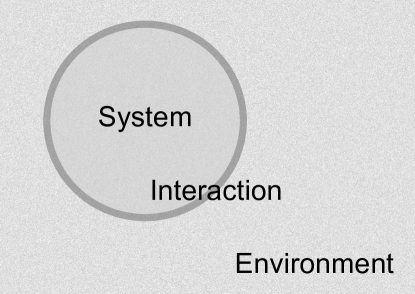
Figure 1: Depiction of a system embedded in its environment, with short-range interactions. The typical argument for neglecting the interaction energy is that in the macroscopic limit the boundary becomes immeasurable in relation to the bulk.

These conditions are customarily achieved by assuming short-range interactions and a relatively large system size, see Fig. (1). However this assumption is generally not justifiable for small systems as Fig. (2) suggests. In this paper, we address the stationary state of open quantum systems in contact with a thermal reservoir at temperature $T=1/\beta$, without the assumption of a vanishing interaction strength and allow for finite relaxation timescales (). Relation (I.1) is known not to hold under these conditions Geva et al. (2000). Phenomenologically, one can estimate the corrections we describe by the ratio of the relaxation rates $\gamma$ to the system’s energy level splittings $\Omega$, or $\gamma/\Omega$.

As thoroughly discussed in Ref. Geva et al. (2000), this fact is often overlooked in many circumstances, due to the effects of ancillary approximations such as the rotating-wave approximation, renormalization of environmentally-induced energy-level shifts and overly-simplistic models. As we explain in Appendix  A, this fact may also be overlooked due to its absence in the case of classical, Gaussian noise.

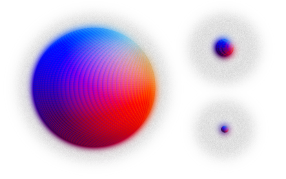
Figure 2: Depiction of systems of decreasing particle number. For systems consisting of a small number particles, the argument in Fig. 1 obviously does not apply. Furthermore, it is known that neglecting the interaction energy in these finite systems always results in infinite relaxation and thermalization times.

Finally, the term equilibrium is used in Ref. Linden et al. (2009) to describe what in our terminology are steady states and in Ref. Reimann (2010) to describe what in our terminology are stationary states. Both cases have been covered in Refs. Short (2011); Short and Farrelly (2012) with the single term equilibrium. These states do necessarily meet our more stringent criteria of equilibrium described above. Here we refer to the result of these works using the terminology we defined above.

I.2 Model and Assumptions

We consider unitary dynamics of the closed system (C) described by the Hamiltonian $\mathbf{H}_{\mathrm{C}}$ consisting of the system of interest (S) and its environment (E) with interaction (I)

$$\mathbf{H}_{\mathrm{C}} =\mathbf{H}_{\mathrm{S}}+\mathbf{H}_{\mathrm{E}}+\mathbf{H}_{\mathrm{I}}+\mathbf{H}_{\mathrm{R}}\,,$$ (I.2)

where $\mathbf{H}_{\mathrm{R}}$ contains all of the “renormalization” (R) effects. The interaction generates environmental correlation functions, c.f. Eqs. (III.4), (III.8)), and we assume these correlations to be decaying functions. This assumption allows for irreversible dynamics in the open system. Implicit in this assumption is that the environment contains a continuum of modes (e.g. infinite volume). This latter assumption can be satisfied by coupling the system directly to field degrees of freedom that are uncountably infinite, such as the electromagnetic field. Note however that we do not assume the interaction Hamiltonian to be negligible compared to the system Hamiltonian.

Finally, for mathematical simplicity we assume the initial state of the system and environment to be uncorrelated at $t=0$

$$\boldsymbol{\rho}_{\mathrm{C}}(0) =\boldsymbol{\rho}_{\mathrm{S}}(0)\otimes\frac{e^{-\beta\mathbf{H}_{\mathrm{E}}}}{Z_{\mathrm{E}}(\beta)}\,,$$ (I.3)

where the environment (a thermal reservoir) is in its isolated equilibrium state with partition function $Z_{\mathrm{E}}(\beta)=\mathrm{Tr_{E}}[e^{-\beta\mathbf{H}_{\mathrm{E}}}]$, and the system (S) is in an arbitrary state.

The assumption of a thermal state for the environment can be justified, for instance, by the approach of Popescu et al. Popescu et al. (2006) in the weak-coupling limit, by giving the environment its own environment, without any restriction on the system-environment coupling strength. In this sense the work of Popescu et al., and those prior, serve as a pedagogical springboard for our analysis of strongly coupled systems.

I.3 Results

It is well known that in the limit of vanishing interaction strength, the open system relaxes to its thermal state van Hove (1954); Davies (1976b); Geva et al. (2000); Fleming and Hu

$$\lim_{\gamma\to 0}\lim_{t\to\infty}\boldsymbol{\rho}_{\mathrm{S}}(t) =\frac{e^{-\beta\mathbf{H}_{\mathrm{S}}}}{Z_{\mathrm{S}}(\beta)}\,,$$ (I.4)

where $\boldsymbol{\rho}_{\mathrm{S}}(t)=\mathrm{Tr}_{\mathrm{E}}[\boldsymbol{\rho}_{\mathrm{C}}(t)]$ denotes the reduced density matrix and $\gamma$ a generic relaxation rate of the open system. Note that all relaxation rates are, at minimum, second order in the interaction, being primarily determined by the two-time correlations of the environment.

In Ref. Mori and Miyashita (2008), it was shown to second-order in the interaction, and for a single tensor-product coupling of system and environment operators, that the open system can be confirmed to relax to the reduced closed system thermal state

$$\lim_{t\to\infty}\boldsymbol{\rho}_{\mathrm{S}}(t) =\mathrm{Tr}_{\mathrm{E}}\!\left[\frac{e^{-\beta\mathbf{H}_{\mathrm{C}}}}{Z_{\mathrm{C}}(\beta)}\right]\,.$$ (I.5)

We extend this proof to general system-environment couplings. For zero-temperature environments we demonstrate agreement with the ground state obtained from the time-independent Schrödinger equation. Moreover, we give a non-perturbative proof of Eq. (I.5) for the exactly-solvable model of $N$-oscillator quantum Brownian motion (N-QBM), wherein the interacting system and environment are linear. In that model we are also able to rigorously prove that all multi-time correlations of the open system relax to those of the closed system thermal state with non-vanishing interaction. Correspondence of the multi-time correlations is an important consideration as, outside of the Markovian regime, the dynamics of the multi-time correlations cannot be generated by the dynamics of the single-time correlations, as per the quantum regression theorem (QRT) Swain (1981).

The reduced, closed system thermal state

It is important to emphasize that Eq. (I.5) pertains strictly to the open system S and not to the closed system (S + E), as equilibration requires not only a reservoir and late-time limit, but also a degree of coarse graining. As we show in Sec. II.6, if one considers any individual mode of the environment, then its dependence upon the initial state of the system never decays. In this sense, information pertaining to the system’s past is encoded in the environment, but only when considering the state of the closed system (S + E). However, upon coarse graining the environment by considering the time-evolution of a continuum of environment energies, and not one individual mode energy, then all dependence upon the initial state of the system is seen to decay away in time. In this sense, information pertaining to the system’s past is only measurable for a finite span of time.

The above statement is based on the fact that, while the open system experiences irreversible dynamics: dissipation, diffusion and decoherence, the closed system (S + E) experiences reversible dynamics. Consider, for instance, the coupling of a mixed state of the system to a zero-temperature reservoir. Given unitary dynamics, the joint state of the system and environment cannot relax from a mixed state into a pure state (the ground state of the interacting theory). However, the environment is exceedingly large when compared to the system, and so the system’s entropy, when spread out over every mode of the environment, can become immeasurable. This is a general phenomena of environmentally-induced irreversible dynamics: conserved quantities such as energy and entropy can flow into the environment, and owing to the overwhelmingly large number of degrees of freedom, become difficult to track or retrieve.

The paper is organized as follows: In Sec. II we derive the equilibrium state for the linear N-QBM model. In Sec. III we extend our analysis to nonlinear systems via perturbation theory. In Sec. IV we summarize our results and compare them to relevant works in the literature and provide some new insights into the key issues. Some technical details have been provided and the notation is defined in the Appendices.

II Linear systems

II.1 The Lagrangian

Our treatment of the N-QBM model is based on Fleming et al. (2011b). The model is that of a continuous and linear system with finite and countable degrees of freedom, with Lagrangian $L_{\mathrm{sys}}(\mathbf{X},\dot{\mathbf{X}})$, bilinearly coupled, via a Lagrangian $L_{\mathrm{int}}(\mathbf{X},\mathbf{x})$, to a linear environment with an infinite (and possibly continuous) number of degrees of freedom, with Lagrangian $L_{\mathrm{env}}(\mathbf{x},\dot{\mathbf{x}})$.

$$L= \;L_{\mathrm{sys}}(\mathbf{X},\dot{\mathbf{X}})+L_{\mathrm{env}}(\mathbf{x},\dot{\mathbf{x}})+L_{\mathrm{int}}(\mathbf{X},\mathbf{x})+L_{\mathrm{ren}}(\mathbf{X})\,,$$ (II.1)

$$L= \;\frac{1}{2}\left(\dot{\mathbf{X}}^{\mathrm{T}}\mathbf{M}\,\dot{\mathbf{X}}-\mathbf{X}^{\mathrm{T}}\mathbf{C}\,\mathbf{X}\right)+\frac{1}{2}\left(\dot{\mathbf{x}}^{\mathrm{T}}\mathbf{m}\,\dot{\mathbf{x}}-\mathbf{x}^{\!\mathrm{T}}\mathbf{c}\,\mathbf{x}\right)$$

$$-\mathbf{x}^{\!\mathrm{T}}\mathbf{g}\,\mathbf{X}+L_{\mathrm{ren}}(\mathbf{X})\,.$$ (II.2)

We assume that the spring constant matrices $\mathbf{C},\mathbf{c}$ as well as the mass matrices $\mathbf{M},\mathbf{m}$ are real and positive definite, and can be considered in general to be symmetric. If necessary, one can relax the positivity condition and even consider time-dependent mass matrices, spring constant matrices and system environment coupling matrix $\mathbf{g}$ Fleming . Such a model environment can emulate any source of Gaussian noise with proper choice of coupling. To ensure that the free and interacting system are similar in behavior, we will also include the “renormalization” $L_{\mathrm{ren}}(\mathbf{X})$. Our choice of “renormalization” will be equivalent to inserting the entire system-environment interaction in the square of the potential:

$$L= \;\frac{1}{2}\left(\dot{\mathbf{X}}^{\mathrm{T}}\mathbf{M}\,\dot{\mathbf{X}}-\mathbf{X}^{\mathrm{T}}\mathbf{C}\,\mathbf{X}\right)$$

$$+\frac{1}{2}\left(\dot{\mathbf{x}}^{\mathrm{T}}\mathbf{m}\,\dot{\mathbf{x}}-\left[\mathbf{x}-\mathbf{c}^{-1}\mathbf{g}\,\mathbf{X}\right]^{\mathrm{T}}\!\!\mathbf{c}\left[\mathbf{x}-\mathbf{c}^{-1}\mathbf{g}\,\mathbf{X}\right]\right),$$ (II.3)

since this keeps the phenomenological system-system couplings from changing.

II.2 The Langevin Equation

For the linear system there are several formalisms which produce the same Langevin Equation. The most direct is via integrating out environment degrees of freedom in the Heisenberg equations of motion Ford et al. (1988) and then considering the symmetrized moments. Another is to consider the characteristic curves of the system + environment’s Fokker-Plank equation Fleming . Finally, one can integrate out both the environment degrees of freedom and the relative system coordinate $\boldsymbol{\Delta}=\mathbf{X}-\mathbf{X}^{\prime}$, while leaving only the average system coordinate $\boldsymbol{\Sigma}=(\mathbf{X}+\mathbf{X}^{\prime})/2$, in the double path integral of the reduced system propagator in the influence functional formalism Calzetta et al. (2003). In general (for nonlinear systems) there is no necessary correspondence between these formalisms and only the first may be well defined, but here the Langevin equation is simply

$$\mathbf{M}\,\ddot{\mathbf{X}}(t)+2\!\int_{0}^{t}\!\!\mathrm{d}s\,\boldsymbol{\gamma}(t,s)\,\dot{\mathbf{X}}(s)+\mathbf{C}\,\mathbf{X}(t) =\boldsymbol{\xi}(t)-2\,\boldsymbol{\gamma}(t)\,\mathbf{X}_{0}\,,$$ (II.4)

where $\boldsymbol{\gamma}$ is the damping kernel and $\boldsymbol{\xi}$ is the noise given by:

$$\boldsymbol{\gamma}(t,s) =+\mathbf{g}^{\mathrm{T}}\mathbf{m}^{\!-\frac{1}{2}}\frac{\cos\!\left(\boldsymbol{\omega}[t\!-\!s]\right)}{2\,\boldsymbol{\omega}^{2}}\mathbf{m}^{\!-\frac{1}{2}}\mathbf{g}\,,$$ (II.5)

$$\boldsymbol{\xi}(t) =\mathbf{g}^{\mathrm{T}}\left(\dot{\mathbf{f}}(t)\,\mathbf{m}\,\mathbf{x}_{0}+\mathbf{f}(t)\,\mathbf{p}_{0}\,\right)\,,$$ (II.6)

$$\mathbf{f}(t) =\mathbf{m}^{-\frac{1}{2}}\frac{\sin(\boldsymbol{\omega}t)}{\boldsymbol{\omega}}\mathbf{m}^{-\frac{1}{2}}\,,$$ (II.7)

$$\boldsymbol{\omega}^{2} \equiv\mathbf{m}^{\!-\frac{1}{2}}\mathbf{c}\,\mathbf{m}^{\!-\frac{1}{2}}\,,$$ (II.8)

where $\mathbf{f}$ is the free Green’s function of the reservoir positions and $\boldsymbol{\omega}$ is the free reservoir frequencies upon diagonalization. Note that the damping kernel is independent of the environment’s initial state, whereas the properties of noise are determined by the environment’s initial state.

We consider the case in which the system and environment are uncorrelated at $t=0$ and the environment is in its thermal state $e^{-\beta\mathbf{H}_{\mathrm{E}}}/Z_{\mathrm{E}}(\beta)$. The noise has zero mean and the two time correlation is given by the noise kernel

$$\boldsymbol{\nu}(t,t^{\prime})=\left\langle\boldsymbol{\xi}(t)\,\boldsymbol{\xi}(t^{\prime})^{\mathrm{T}}\right\rangle_{\boldsymbol{\xi}}\,,$$ (II.9)

where the Gaussian average over the stochastic process $\boldsymbol{\xi}$ is equivalent to tracing over the environment degrees of freedom. The noise and damping kernels satisfy then the fluctuation-dissipation relation (here in the Fourier domain)

$$\tilde{\boldsymbol{\nu}}(\omega) =\tilde{\kappa}(\omega)\,\tilde{\boldsymbol{\gamma}}(\omega)\,,$$ (II.10)

$$\tilde{\kappa}(\omega) \equiv\hbar\omega\,\coth\!\left(\frac{\hbar\omega}{2k_{\mathrm{B}}T}\right)\,,$$ (II.11)

with the Fourier transform defined

$$\tilde{f}(\omega)\equiv\int_{\!-\infty}^{+\infty}\!\!\!\mathrm{d}t\,e^{-\imath\omega t}\,f(t)\,,$$ (II.12)

and where $\tilde{\kappa}$ is the (quantum) FDR kernel. Therefore, the problem is completely specified in terms of the damping kernel.

Given that our damping kernel is stationary, the Langevin equation can be expressed in the Laplace domain as

$$\left[z^{2}\mathbf{M}+2z\hat{\boldsymbol{\gamma}}(z)+\mathbf{C}\right]\hat{\mathbf{X}}(z) =[z\mathbf{M}\,\mathbf{X}_{0}+\mathbf{P}_{0}]+\hat{\boldsymbol{\xi}}(z)\,,$$ (II.13)

where $\mathbf{P}=\mathbf{M}\,\dot{\mathbf{X}}$ and $(\mathbf{X}_{0},\mathbf{P}_{0})$ correspond to the initial values at $t=0$, and with the Laplace transform defined

$$\hat{f}(z)\equiv\int_{0}^{\infty}\!\!\mathrm{d}t\,e^{-zt}\,f(t)\,.$$ (II.14)

Formally, the solutions can be easily found by inversion:

$$\hat{\mathbf{X}}(z) =\hat{\mathbf{G}}(z)\,[z\mathbf{M}\,\mathbf{X}_{0}+\mathbf{P}_{0}]+\hat{\mathbf{G}}(z)\,\hat{\boldsymbol{\xi}}(z)\,,$$ (II.15)

$$\hat{\mathbf{G}}(z) =\left[z^{2}\mathbf{M}+2z\hat{\boldsymbol{\gamma}}(z)+\mathbf{C}\right]^{-1}\,.$$ (II.16)

Note that since our damping kernel is symmetric, i.e. $\boldsymbol{\gamma}(t,s)=\boldsymbol{\gamma}(t,s)^{\mathrm{T}}$, the same will be true for the propagator $\mathbf{G}(t,s)$ and its Laplace transform. It is also useful to consider the following representation:

$$\hat{\mathbf{G}}(z) =\mathbf{M}^{-\frac{1}{2}}\left[z^{2}+2z\,\hat{\boldsymbol{\lambda}}(z)+\boldsymbol{\Omega}^{2}\right]^{-1}\mathbf{M}^{-\frac{1}{2}}\,,$$ (II.17)

$$\hat{\boldsymbol{\lambda}}(z) \equiv\mathbf{M}^{-\frac{1}{2}}\hat{\boldsymbol{\gamma}}(z)\,\mathbf{M}^{-\frac{1}{2}}\,,$$ (II.18)

$$\boldsymbol{\Omega}^{2} \equiv\mathbf{M}^{-\frac{1}{2}}\mathbf{C}\,\mathbf{M}^{-\frac{1}{2}}\,,$$ (II.19)

where the eigenvalues of $\boldsymbol{\Omega}^{2}$ coincide with the squared frequencies of the normal modes of the free system. Back in the time domain we have

$$\mathbf{X}(t) =\dot{\mathbf{G}}(t)\,\mathbf{M}\,\mathbf{X}_{0}+\mathbf{G}(t)\,\mathbf{P}_{0}+(\mathbf{G}*\boldsymbol{\xi})(t)\,,$$ (II.20)

with $*$ denoting the Laplace convolution, defined as

$$(A*B)(t)=\int_{0}^{t}\!\!\mathrm{d}s\,A(t\!-\!s)\,B(s).$$ (II.21)

For more general Gaussian states, for which the system and environment are correlated, the noise can be correlated with $(\mathbf{X}_{0},\mathbf{P}_{0})$ and the noise kernel modified. This is the case for the closed system thermal state given by the density matrix $e^{-\beta\mathbf{H}_{\mathrm{C}}}/Z_{\mathrm{C}}(\beta)$ which we investigate below.

II.3 Single-time correlations in the closed system thermal state

In this section we calculate the single-time correlations in the closed system thermal state of the N-QBM model. The partition function for the N-QBM model has been derived in App. C, Eq. (C.17). In the rest of the paper including the appendices we suppress the dependence of the paritition function on $\beta$ for brevity of notation. As a first step we take the logarithm of the partition function and write it as:

$$\log Z_{\mathrm{C}} =\log Z_{\mathrm{E}}-\frac{1}{2}\mathrm{Tr}\log\mathbf{M}^{-1}-\frac{1}{2}\mathrm{Tr}\log\mathbf{C}$$

$$-\sum_{r=1}^{\infty}\mathrm{Tr}\log\left(\mathbf{M}^{-1}\hat{\mathbf{G}}(\nu_{\mathrm{r}})^{-1}\right)+\mathrm{constant}$$ (II.22)

We begin by making a general observation. Consider the thermal state of a system described by a Hamiltonian where the momenta appear only in the kinetic energy term of the form $\sum_{a}p_{a}^{2}/2m$. Then all correlations between position and momentum operators vanish: $\left\langle x_{a}p_{b}\right\rangle=0$. This can be seen by noting that all correlations are time-translation-invariant in equilibrium and forming the derivatives $\frac{\mathrm{d}}{\mathrm{d}t}\left\langle x_{a}(t)x_{b}(t)\right\rangle$ and $\frac{\mathrm{d}}{\mathrm{d}(t-t^{\prime})}\left\langle x_{a}(t)x_{b}(t^{\prime})\right\rangle\big{|}_{t=t^{\prime}}$. This observation applies to N-QBM model.

Let angular bracket with the subscript C denote expectation values in the closed system thermal state. Expectation values corresponding to the uncorrelated initial state are denoted by attaching the subscript E to the bracket. For the purpose of partial differentiation, the partition function is to be regarded as a function of $\mathbf{C},\ \mathbf{M},\ \mathbf{c},\ \mathbf{m},\ \mathbf{g}$ and not (explicitly) of $\boldsymbol{\omega}$. With a straight-forward application of Theorem 1, the reduced system correlations are given by:

$$\left\langle\mathbf{X}\,\mathbf{X}^{\mathrm{T}}\right\rangle_{\mathrm{C}} =-\frac{2}{\beta}\frac{\partial\log Z_{\mathrm{C}}}{\partial\mathbf{C}}\,,$$ (II.23)

$$\left\langle\mathbf{X}\,\mathbf{P}^{\mathrm{T}}\right\rangle_{\mathrm{C}} =\left\langle\mathbf{P}\,\mathbf{X}^{\mathrm{T}}\right\rangle=0\,,$$ (II.24)

$$\left\langle\mathbf{P}\,\mathbf{P}^{\mathrm{T}}\right\rangle_{\mathrm{C}} =-\frac{2}{\beta}\frac{\partial\log Z_{\mathrm{C}}}{\partial\mathbf{M}^{-1}}\,.$$ (II.25)

The position-position and position-momentum correlations between system and reservoir modes are calculated similarly:

$$\left\langle\mathbf{X}\,\mathbf{x}^{\mathrm{T}}\right\rangle_{\mathrm{C}} =\left\langle\mathbf{x}\,\mathbf{X}^{\mathrm{T}}\right\rangle_{\mathrm{C}}^{\mathrm{T}}$$ (II.26)

$$=\frac{1}{\beta}\frac{\partial\log Z_{C}}{\partial\mathbf{g}^{\mathrm{T}}}+\left\langle\mathbf{X}\,\mathbf{X}^{\mathrm{T}}\right\rangle_{\mathrm{C}}\,\mathbf{g}^{\mathrm{T}}\mathbf{c}^{-1}\,,$$

$$\left\langle\mathbf{X}\,\mathbf{p}^{\mathrm{T}}\right\rangle_{\mathrm{C}} =\left\langle\mathbf{p}\,\mathbf{X}^{\mathrm{T}}\right\rangle_{\mathrm{C}}^{\mathrm{T}}=0\,,$$ (II.27)

$$\left\langle\mathbf{P}\,\mathbf{x}^{\mathrm{T}}\right\rangle_{\mathrm{C}} =\left\langle\mathbf{x}\,\mathbf{P}^{\mathrm{T}}\right\rangle_{\mathrm{C}}^{\mathrm{T}}=0\,.$$ (II.28)

To calculate the momentum-momentum correlations between system and environment we take the time derivative of $\left\langle\mathbf{X}(t)\mathbf{p}^{\mathrm{T}}(t)\right\rangle_{\mathrm{C}}$ and set it to zero. Since in the closed system thermal state all expectation values are time-independent, we know that there is in fact no dependence on time. Using the equations of motion it is straight-forward to show that:

$$\left\langle\mathbf{P}\,\mathbf{p}^{\mathrm{T}}\right\rangle_{\mathrm{C}} =\mathbf{M}\,\left\langle\mathbf{X}\,\mathbf{x}^{\mathrm{T}}\right\rangle_{\mathrm{C}}\,\mathbf{c}-\mathbf{M}\,\left\langle\mathbf{X}\,\mathbf{X}^{\mathrm{T}}\right\rangle_{\mathrm{C}}\,\mathbf{g}^{\mathrm{T}}\,.$$ (II.29)

The environment correlations can be calculated by direct differentiation of the partition function:

$$\left\langle\mathbf{x}\,\mathbf{x}^{\mathrm{T}}\right\rangle_{\mathrm{C}} =-\frac{2}{\beta}\frac{\partial\log Z_{C}}{\partial\mathbf{c}}+\mathbf{c}^{-1}\mathbf{g}\,\left\langle\mathbf{X}\,\mathbf{X}^{\mathrm{T}}\right\rangle_{\mathrm{C}}\,\mathbf{g}^{\mathrm{T}}\mathbf{c}^{-1}\,,$$ (II.30)

$$\left\langle\mathbf{x}\,\mathbf{p}^{\mathrm{T}}\right\rangle_{\mathrm{C}} =\left\langle\mathbf{p}\,\mathbf{x}^{\mathrm{T}}\right\rangle_{\mathrm{C}}=0\,,$$ (II.31)

$$\left\langle\mathbf{p}\,\mathbf{p}^{\mathrm{T}}\right\rangle_{\mathrm{C}} =-\frac{2}{\beta}\frac{\partial\log Z_{C}}{\partial\mathbf{m}^{-1}}\,.$$ (II.32)

Now we are in a position to determine all the single-time correlations of the interacting theory in the closed system thermal state. Since the equilibrium state is stationary these single-time correlations are time-independent. The details for some of these formulae are provided in App D. All the nonzero correlations are given by:

$$\left\langle\mathbf{X}\,\mathbf{X}^{\mathrm{T}}\right\rangle_{\mathrm{C}} =\frac{1}{\beta}\hat{\mathbf{G}}(\nu_{0})+\frac{2}{\beta}\sum_{r=1}^{\infty}\hat{\mathbf{G}}(\nu_{\mathrm{r}})\,,$$ (II.33)

$$\left\langle\mathbf{P}\,\mathbf{P}^{\mathrm{T}}\right\rangle_{\mathrm{C}} =\frac{1}{\beta}\left(\mathbf{M}-\nu_{0}^{2}\mathbf{M}\,\hat{\mathbf{G}}(\nu_{0})\,\mathbf{M}\right)$$ (II.34)

$$+\frac{2}{\beta}\sum_{\mathrm{r}=1}^{\infty}\left(\mathbf{M}-\nu_{\mathrm{r}}^{2}\mathbf{M}\,\hat{\mathbf{G}}(\nu_{\mathrm{r}})\,\mathbf{M}\right)\,,$$

$$\left\langle\mathbf{X}\,\mathbf{x}^{\mathrm{T}}\right\rangle_{\mathrm{C}} =\left\langle\mathbf{X}\,\mathbf{X}^{\mathrm{T}}\right\rangle_{\mathrm{C}}\mathbf{g}^{\mathrm{T}}\mathbf{c}^{-1}-\frac{2}{\beta}\sum_{r=1}^{\infty}\nu_{\mathrm{r}}\hat{\mathbf{G}}(\nu_{\mathrm{r}})\,\hat{\boldsymbol{\gamma}}(\nu_{\mathrm{r}})\,\mathbf{g}^{-1}\,,$$ (II.35)

$$\left\langle\mathbf{P}\,\mathbf{p}^{\mathrm{T}}\right\rangle_{\mathrm{C}} =\mathbf{M}\left\langle\mathbf{X}\,\mathbf{x}^{\mathrm{T}}\right\rangle_{\mathrm{C}}\mathbf{c}-\mathbf{M}\left\langle\mathbf{X}\mathbf{X}^{\mathrm{T}}\right\rangle_{\mathrm{C}}\mathbf{g}^{\mathrm{T}}\,,$$ (II.36)

$$\left\langle\mathbf{p}_{0}\,\mathbf{p}_{0}^{\mathrm{T}}\right\rangle_{\mathrm{C}} =\left\langle\mathbf{p}_{0}\,\mathbf{p}_{0}^{\mathrm{T}}\right\rangle_{\mathrm{E}}$$ (II.37)

$$-\frac{2}{\beta}\sum_{\mathrm{r}=1}^{\infty}\nu_{\mathrm{r}}^{2}\mathbf{m}\,\hat{\mathbf{f}}(\nu_{\mathrm{r}})\,\mathbf{g}\,\hat{\mathbf{G}}(\nu_{\mathrm{r}})\,\mathbf{g}^{\mathrm{T}}\hat{\mathbf{f}}(\nu_{\mathrm{r}})\,\mathbf{m}\,,$$

$$\left\langle\mathbf{x}_{0}\,\mathbf{x}_{0}^{\mathrm{T}}\right\rangle_{\mathrm{C}} =\left\langle\mathbf{x}_{0}\,\mathbf{x}_{0}^{\mathrm{T}}\right\rangle_{\mathrm{E}}+\mathbf{c}^{-1}\mathbf{g}\left\langle\mathbf{X}_{0}\,\mathbf{X}\right\rangle_{\mathrm{C}}\mathbf{g}^{\mathrm{T}}\mathbf{c}^{-1}$$ (II.38)

$$-\frac{2}{\beta}\sum_{\mathrm{r}=1}^{\infty}\nu_{\mathrm{r}}^{2}\left(\mathbf{c}^{-1}\mathbf{m}\,\hat{\mathbf{f}}(\nu_{\mathrm{r}})\,\mathbf{g}\,\hat{\mathbf{G}}(\nu_{\mathrm{r}})\,\mathbf{g}^{\mathrm{T}}\hat{\mathbf{f}}(\nu_{\mathrm{r}})\right)$$

$$-\frac{2}{\beta}\sum_{\mathrm{r}=1}^{\infty}\nu_{\mathrm{r}}^{2}\left(\hat{\mathbf{f}}(\nu_{\mathrm{r}})\,\mathbf{g}\,\hat{\mathbf{G}}(\nu_{\mathrm{r}})\,\mathbf{g}^{\mathrm{T}}\hat{\mathbf{f}}(\nu_{\mathrm{r}})\,\mathbf{m}\,\mathbf{c}^{-1}\right)$$

$$-\frac{2}{\beta}\sum_{\mathrm{r}=1}^{\infty}\nu_{\mathrm{r}}^{4}\left(\mathbf{c}^{-1}\mathbf{m}\,\hat{\mathbf{f}}(\nu_{\mathrm{r}})\,\mathbf{g}\,\hat{\mathbf{G}}(\nu_{\mathrm{r}})\,\mathbf{g}^{\mathrm{T}}\hat{\mathbf{f}}(\nu_{\mathrm{r}})\,\mathbf{m}\,\mathbf{c}^{-1}\right),$$

where $\hat{\mathbf{f}}$ is the Laplace transform of the free reservoir propagator given by Eq. (II.7) and $\nu_{\mathrm{r}}=2\pi\mathrm{r}/\hbar\beta$ are the Matsubara frequencies.

II.4 Equivalence of single-time correlations for the open system

In this subsection we show that the single-time correlations of system variables for the uncorrelated initial state are asymptotically identical to the single-time correlations corresponding to the closed system thermal state. We start by calculating the variances for the closed system thermal state. The requirement that $\mathbf{G}(t)$ is a decaying function means that the Laplace transform $\hat{\mathbf{G}}(z)$ is analytic in the right half-plane. Hence $\hat{\mathbf{G}}(-\imath\omega)$ is analytic in the upper-half plane. On the other hand $\coth(\beta\hbar\omega/2)$ has simple poles on the imaginary axis at the Matzubara frequencies $\nu_{\mathrm{r}}$. The summations over $r$ in Eq. (II.33) can be written as a contour integral using Cauchy’s theorem:

$$\left\langle\mathbf{X}\,\mathbf{X}^{\mathrm{T}}\right\rangle_{\mathrm{C}} =\frac{\beta\hbar/2}{2\pi\imath}\times\frac{2}{\beta}\int_{C}\mathrm{d}z\coth(\beta\hbar z/2)\,\hat{\mathbf{G}}(-\imath z)\,.$$ (II.39)

The contour of integration is chosen to encircle the upper-half plane in a counter-clockwise direction. The poles on the imaginary axis at Matzubara frequencies $\nu_{\mathrm{r}}$ for $r\geq 1$ are encircled, but only half of the pole at the origin is enclosed. The arc of the contour does not contribute to the integral when the radius is taken to infinity. Hence we can write this expression as an integral on the real line. Furthermore, by the symmetry of the integrand, the real part vanishes and the integral is given by:

$$\left\langle\mathbf{X}\,\mathbf{X}^{\mathrm{T}}\right\rangle_{\mathrm{C}} =\frac{\hbar}{2\pi}\int_{\!-\infty}^{+\infty}\!\!\!\mathrm{d}\omega\coth(\beta\hbar\omega/2)\,\mathrm{Im}\!\left[\hat{\mathbf{G}}(-\imath\omega)\right].$$ (II.40)

A similar argument can be used to derive:

$$\left\langle\mathbf{P}\,\mathbf{P}^{\mathrm{T}}\right\rangle_{\mathrm{C}} =\frac{\hbar}{2\pi}\int_{\!-\infty}^{+\infty}\!\!\!\mathrm{d}\omega\,\omega^{2}\coth(\beta\hbar\omega/2)\,\mathrm{Im}\!\left[\hat{\mathbf{G}}(-\imath\omega)\right].$$ (II.41)

Eqs. (II.40,II.41) are identical to the results obtained by Fleming et al. (2011b) for the asymptotic values of variances corresponding to an uncorrelated initial state. Therefore we have proven that the single-time correlations of the open system relax to those of the closed system thermal state.

II.5 Equivalence of multi-time correlations

In this section we generalize the results of the previous section to include multi-time correlations. We begin by calculating the two-time correlation function $\left\langle\mathbf{X}(t)\,\mathbf{X}(t^{\prime})^{\mathrm{T}}\right\rangle_{\mathrm{C}}$ using the trajectories obtained from the Langevin equation. Note that for the closed system thermal state this quantity is stationary. To simplify the proof we make use of this observation and take the late-time limit of the closed system thermal state as well without loss of generality. This trick makes the comparison of the two cases easier and reduces the amount of computation.

The dynamics of the system is given by the solution (II.20) of the Langevin equation which is valid for any initial state. The dependence on initial state is hidden in the correlations between $\mathbf{X}_{0},\ \mathbf{P}_{0}$ and $\boldsymbol{\xi}(t)$. The two-time position correlation is given by

$$\left\langle\mathbf{X}(t)\,\mathbf{X}(t^{\prime})^{\mathrm{T}}\right\rangle_{\mathrm{C}} =\dot{\mathbf{G}}(t)\,\mathbf{M}\left\langle\mathbf{X}_{0}\,\mathbf{X}_{0}^{\mathrm{T}}\right\rangle_{\mathrm{C}}\mathbf{M}\,\dot{\mathbf{G}}(t^{\prime})+\mathbf{G}(t)\left\langle\mathbf{P}_{0}\,\mathbf{P}_{0}^{\mathrm{T}}\right\rangle_{\mathrm{C}}\mathbf{G}^{\mathrm{T}}(t^{\prime})$$

$$+\dot{\mathbf{G}}(t)\,\mathbf{M}\int_{0}^{t^{\prime}}\!\!\mathrm{d}s^{\prime}\,\left\langle\mathbf{X}_{0}\,\boldsymbol{\xi}(s^{\prime})^{\mathrm{T}}\right\rangle_{\mathrm{C}}\mathbf{G}(t^{\prime}\!-\!s^{\prime})+\int_{0}^{t}\!\!\mathrm{d}s\,\mathbf{G}(t\!-\!s)\left\langle\boldsymbol{\xi}(s)\,\mathbf{X}_{0}^{\mathrm{T}}\right\rangle_{\mathrm{C}}\mathbf{M}\,\dot{\mathbf{G}}(t^{\prime})$$

$$+\mathbf{G}(t)\int_{0}^{t^{\prime}}\!\!\mathrm{d}s^{\prime}\,\left\langle\mathbf{P}_{0}\,\boldsymbol{\xi}(s^{\prime})^{\mathrm{T}}\right\rangle_{\mathrm{C}}\mathbf{G}(t^{\prime}\!-\!s^{\prime})+\int_{0}^{t}\!\!\mathrm{d}s\,\mathbf{G}(t\!-\!s)\left\langle\boldsymbol{\xi}(s)\,\mathbf{P}_{0}^{\mathrm{T}}\right\rangle_{\mathrm{C}}\dot{\mathbf{G}}(t^{\prime})$$

$$+\int_{0}^{t}\!\!\mathrm{d}s\int_{0}^{t^{\prime}}\!\!\mathrm{d}s^{\prime}\,\mathbf{G}(t\!-\!s)\left\langle\boldsymbol{\xi}(s)\,\boldsymbol{\xi}(s^{\prime})^{\mathrm{T}}\right\rangle_{\mathrm{C}}\mathbf{G}(t^{\prime}\!-\!s^{\prime})\,.$$ (II.42)

As mentioned earlier unlike the uncorrelated initial state the terms in the second and third lines do not vanish in the closed system thermal state. We consider the case where

$$\lim_{t\rightarrow\infty}\mathbf{G}(t)=\lim_{t\rightarrow\infty}\boldsymbol{\gamma}(t)=0\,.$$ (II.43)

This is the criteria for dissipative dynamics. Under these assumptions the first two terms in Eq. (II.42) vanish in the late-time limit for any initial state. The terms in the second and third lines have one factor of $\mathbf{G}(t)$ or $\dot{\mathbf{G}}(t)$ that goes to zero in the late-time limit multiplied by a convolution integral. In App. D we show that these convolution integrals are finite. Hence the terms in second and third lines also vanish asymptotically. Finally we show the equivalence of the term in the last line for the uncorrelated and thermal initial states at late times in App. E.

The comparison of more general multi-time correlations can be done similarly using the trajectories of the Langevin equation. The above example demonstrates how in the late-time limit the effects of initial conditions of the system die out and the noise statistics of both preparations converge. The equivalence at the level of trajectories ensures that all the multi-time correlations will be identical.

Let us reiterate the result we just obtained: a linear system linearly coupled to a linear thermal reservoir (with uncountably many degrees of freedom) at inverse temperature $\beta$ does relax to the equilibrium state described by (I.5). This state is different from the Boltzmann state given by (I.4) whenever the interaction between the system and environment is not negligible. Moreover the multi-time correlations of system observables also relax to their corresponding values in the closed system thermal state.

II.6 The effect of coarse graining

Up until this point we only focused on the system degrees of freedom. Now we turn our attention to the environment. Following Ref. Fleming et al. (2011b); Fleming , the trajectories of the environment oscillators, as driven by the system oscillators, are given by

$$\mathbf{x}(t) =\left[\dot{\mathbf{f}}(t)\,\mathbf{m}\,\mathbf{x}(0)+\mathbf{f}(t)\,\mathbf{p}(0)\right]+\mathbf{f}(t)*\mathbf{g}\,\mathbf{X}(t)\,,$$ (II.44)

in terms of their free propagator $\mathbf{f}(t)$ and frequency matrix $\boldsymbol{\omega}$ given by Eqs. (II.7,II.8). Into Eq. (II.44) we substitute the system trajectories, which are damped oscillations driven by noise for the continuum environment:

$$\mathbf{X}(t) =\left[\dot{\mathbf{G}}(t)\,\mathbf{M}\,\mathbf{X}(0)+\mathbf{G}(t)\,\mathbf{P}(0)\right]+\mathbf{G}(t)*\boldsymbol{\xi}(t)\,.$$ (II.45)

We then find the environmental dependence upon the initial state of the system to be

$$\mathbf{x}(t) =\mathbf{f}(t)\,\mathbf{g}*\left[\dot{\mathbf{G}}(t)\,\mathbf{M}\,\mathbf{X}(0)+\mathbf{G}(t)\,\mathbf{P}(0)\right]+\cdots\,,$$ (II.46)

with all additional terms only dependent upon the initial state of the environment. The system-dependent terms correspond to a convolution of harmonic oscillations of the environment with non-locally damped oscillations of the system. Resolving these integrals leads to some terms which oscillate with environment frequencies $\omega$ and do not decay.

As a simple example, consider the local damping of a single system oscillator. The open-system propagator or Green’s function is given by

$$G(t) =\frac{\sin(\tilde{\Omega}t)}{M\tilde{\Omega}}e^{-\gamma_{0}t}\,,$$ (II.47)

$$\tilde{\Omega} =\sqrt{\Omega^{2}-\gamma_{0}^{2}}\,.$$ (II.48)

The environment’s dependence upon the initial state of the system is given by

$$x_{k}(t)= \left\{X(0)\frac{\mathrm{d}}{\mathrm{d}t}+\frac{P(0)}{M}\right\}\left\{\frac{\mathrm{d}^{2}}{\mathrm{d}t^{2}}-2\gamma_{0}\frac{\mathrm{d}}{\mathrm{d}t}+\Omega^{2}\right\}h_{k}(t)$$

$$+\,\cdots\,,$$ (II.49)

$$h_{k}(t)\equiv \frac{g_{k}f_{k}(t)}{\left(\omega_{k}^{2}-\Omega^{2}\right)^{2}+4\gamma_{0}^{2}\omega_{k}^{2}}\,,$$ (II.50)

plus terms that decay exponentially and the terms which depend upon the initial state of the environment. The function $h_{k}(t)$ oscillates forever, the same as $f_{k}(t)$, and therefore the environment retains information pertaining to the initial state of the system forever. However, this information is not measurable forever. The system only interacts with the integrated trajectories, which resolve to a convolution of the damping kernel and open-system propagators.

$$\mathbf{g}^{\mathrm{T}}\mathbf{x}(t) =-2\,\dot{\boldsymbol{\gamma}}(t)*\left[\dot{\mathbf{G}}(t)\,\mathbf{M}\,\mathbf{X}(0)+\mathbf{G}(t)\,\mathbf{P}(0)\right]+\cdots\,,$$ (II.51)

and upon integrating over a continuum of environment frequencies (here performed by multiplication with the infinite matrix $\mathbf{g}^{\mathrm{T}}$) the oscillatory terms decay in time. Thus the late-time limit and coarse graining together are responsible for the erasure of all information pertaining to the initial state of the system.

III General systems

III.1 Steady state

The time-evolution of the reduced density matrix of the open system can be generated by a perturbative master equation

$$\dot{\boldsymbol{\rho}}_{\mathrm{S}}(t) =\boldsymbol{\mathcal{L}}(t)\!\left\{\boldsymbol{\rho}_{\mathrm{S}}(t)\right\},$$ (III.1)

where the Liouville operator can be expanded in terms of the interaction Hamiltonian by a variety of methods Kampen and Oppenheim (1997); Breuer et al. (2003); Strunz and Yu (2004); Fleming and Hu .

$$\boldsymbol{\mathcal{L}}(t) =\boldsymbol{\mathcal{L}}_{0}+\boldsymbol{\mathcal{L}}_{1}(t)+\boldsymbol{\mathcal{L}}_{2}(t)+\cdots\,,$$ (III.2)

$$\boldsymbol{\mathcal{L}}_{0}\{\boldsymbol{\rho}\} =-\imath[\mathbf{H}_{\mathrm{S}},\boldsymbol{\rho}]\,,$$ (III.3)

In general, $\boldsymbol{\mathcal{L}}_{1}(t)$ can be absorbed into the system Hamiltonian and so we will primarily concern ourselves with the second-order term. For simplicity we will assume there is no degeneracy or near-degeneracy in the system energy spectrum.

Expanding the interaction Hamiltonian in terms of system $\mathbf{L}_{n}$ and environment $\mathbf{l}_{n}$ operators

$$\mathbf{H}_{\mathrm{I}} =\sum_{n}\mathbf{L}_{n}\otimes\mathbf{l}_{n}\,,$$ (III.4)

the multivariate master equation can be represented Fleming and Hu

$$\boldsymbol{\mathcal{L}}_{2}\,\boldsymbol{\rho}=\sum_{nm}\left[\mathbf{L}_{n},\boldsymbol{\rho}\,(\mathbf{A}_{nm}\!\diamond\mathbf{L}_{m})^{\dagger}-(\mathbf{A}_{nm}\!\diamond\mathbf{L}_{m})\,\boldsymbol{\rho}\right]\,,$$ (III.5)

where the $\mathbf{A}$ operators and $\diamond$ product define the second-order operators

$$(\mathbf{A}_{nm}\!\diamond\mathbf{L}_{m})(t)\equiv\int_{0}^{t}\!\!\mathrm{d}s\,\alpha_{nm}(t,s)\,\left\{\boldsymbol{\mathcal{G}}_{0}(t,s)\,\mathbf{L}_{m}(s)\right\}\,,$$ (III.6)

in terms of the zeroth-order (state) propagator of the system

$$\boldsymbol{\mathcal{G}}_{0}(t,s)\{\boldsymbol{\rho}\} =e^{-\imath(t-s)\mathbf{H}_{\mathrm{S}}}\,\boldsymbol{\rho}\,e^{+\imath(t-s)\mathbf{H}_{\mathrm{S}}}\,,$$ (III.7)

and the (multivariate) environmental correlation function

$$\alpha_{nm}(t,s) \equiv \left\langle\underline{\mathbf{l}}_{n}(t)\,\underline{\mathbf{l}}_{m}(s)\right\rangle_{\mathrm{E}}\,.$$ (III.8)

The second-order operator can be expressed as the Hadamard product

$$\left\langle\omega_{i}\right|\mathbf{A}_{nm}\!\diamond\mathbf{L}_{m}\left|\omega_{i^{\prime}}\right\rangle=A(\omega_{i}\!-\!\omega_{i^{\prime}})\,\left\langle\omega_{i}\right|\mathbf{L}_{m}\left|\omega_{i^{\prime}}\right\rangle\,,$$ (III.9)

and, in the late-time limit, the second-order coefficients resolve

$$A_{nm}(\omega) =\frac{1}{2}\tilde{\alpha}_{nm}(\omega)-\imath\,\mathcal{P}\!\left[\frac{1}{\omega}\right]*\tilde{\alpha}_{nm}(\omega)\,,$$ (III.10)

where $\tilde{\boldsymbol{\alpha}}(\omega)$ denotes the Fourier transform of the stationary environment correlation function $\boldsymbol{\alpha}(t-s)=\boldsymbol{\alpha}(t,s)$, $\mathcal{P}$ the Cauchy principal value and $*$ the appropriate Fourier convolution.

With the multivariate master equation detailed, we can prove relation (I.5) to second order in the interaction. This generalizes the univariate proof in Ref. Mori and Miyashita (2008), which considered a single tensor-product interaction between the system and environment. As the proof is straightforward in either case, we will give an outline and focus upon differences which arise in the multivariate treatment.

We are looking for the stationary state $\boldsymbol{\rho}_{\beta}$, such that

$$\boldsymbol{\mathcal{L}}\{\boldsymbol{\rho}_{\beta}\} =0,$$ (III.11)

we know from detailed balance that the zeroth-order stationary state is the thermal state (I.4), e.g. see Fleming and Hu . Second-order corrections can be generated from the second-order master equation via canonical perturbation theory. More explicitly, we have

$$\left\langle\omega_{i}\right|\boldsymbol{\rho}_{\!\beta}\left|\omega_{j}\right\rangle_{i\neq j}\propto e^{-\beta\,\omega_{i}}\,\delta_{ij}-\imath\frac{\left\langle\omega_{i}\right|\boldsymbol{\mathcal{L}}_{2}\{e^{-\beta\,\mathbf{H}}\}\left|\omega_{j}\right\rangle}{\omega_{i}-\omega_{j}}\,,$$ (III.12)

but only for the denoted off-diagonal perturbative corrections (in the energy basis $\left|\omega\right\rangle$). As explained in Ref. Fleming and Cummings (2011), due to unavoidable degeneracy, specifically that the diagonal elements are all stationary to zeroth-order, the second-order master equation cannot determine the second-order corrections to the diagonal elements of the density matrix. Fortunately this does not greatly hamper our proof of correspondence. By a simple application of the multivariate master equation to Eq. (III.12), we easily obtain these second-order corrections to the thermal state of the system.

III.2 Equilibrium state

We wish to compare the straightforward expansion of (III.12) to the reduced closed system thermal state at second order, and so we require a perturbative expansion of (I.5). There exists such a perturbative expansion of exponential matrices utilizing the identity

$$\frac{\mathrm{d}}{\mathrm{d}\epsilon}e^{\mathbf{A}+\epsilon\,\mathbf{B}}=e^{\mathbf{A}+\epsilon\,\mathbf{B}}\!\int_{0}^{1}\!\!\mathrm{d}u\,e^{-u(\mathbf{A}+\epsilon\,\mathbf{B})}\,\mathbf{B}\,e^{+u(\mathbf{A}+\epsilon\,\mathbf{B})}\,,$$ (III.13)

to obtain an operator-Taylor series in the perturbation $\epsilon\,\mathbf{B}$. After a fair amount of simplification, one can determine the second-order stationary state to be

$$\boldsymbol{\rho}_{\!\beta}\propto \;e^{-\beta\,\mathbf{H}_{\mathrm{S}}}$$ (III.14)

$$+e^{-\beta\,\mathbf{H}_{\mathrm{S}}}\!\int_{0}^{\beta}\!\!\mathrm{d}\beta^{\prime}\!\int_{0}^{\beta^{\prime}}\!\!\!\mathrm{d}\beta^{\prime\prime}\left\langle\underline{\mathbf{H}}_{\mathrm{I}}(-\imath\beta^{\prime})\,\underline{\mathbf{H}}_{\mathrm{I}}(-\imath\beta^{\prime\prime})\right\rangle_{\mathrm{E}}\,,$$

in terms of the complex-time operators

$$\underline{\mathbf{H}}_{\mathrm{I}}(-\imath\beta)\equiv e^{+\beta(\mathbf{H}+\mathbf{H}_{\mathrm{E}})}\,\mathbf{H}_{\mathrm{I}}\,e^{-\beta(\mathbf{H}+\mathbf{H}_{\mathrm{E}})}\,,$$ (III.15)

where the noise average is taken with respect to the free thermal state of the environment and factors inside the environmental trace have been written to suggest their correspondence with the environmental correlation function evaluated at imaginary times.

The double integrals in Eq. (III.14) reduce to

$$\sum_{nm}\int_{0}^{\beta}\!\!\!\mathrm{d}\beta^{\prime}\!\int_{0}^{\beta^{\prime}}\!\!\!\mathrm{d}\beta^{\prime\prime}\,\alpha_{nm}(-\imath\beta^{\prime},-\imath\beta^{\prime\prime})\,\underline{\mathbf{L}}_{n}(-\imath\beta^{\prime})\,\underline{\mathbf{L}}_{m}(-\imath\beta^{\prime\prime})\,,$$ (III.16)

in terms of the complex-time operators

$$\underline{\mathbf{L}}(-\imath\beta)\equiv e^{+\beta\,\mathbf{H}_{\mathrm{S}}}\,\mathbf{L}\,e^{-\beta\,\mathbf{H}_{\mathrm{S}}}\,.$$ (III.17)

After a Fourier expansion of the complex-time correlation functions, expressions (III.12) and (III.16) can be compared term-by-term in the energy basis wherein the imaginary-time integrals of Eq. (III.16) can be resolved as the master equation operators were. Though the two expressions will then be composed of the same objects, they will not immediately appear to be equivalent. The final step is to apply the relevant multivariate Kubo-Martin-Schwinger (KMS) relations (also found in Fleming and Hu )

$$\tilde{\boldsymbol{\alpha}}(+\omega)=\tilde{\boldsymbol{\alpha}}^{\!\mathrm{T}\!}(-\omega)\,e^{-\frac{\omega}{T}}=\tilde{\boldsymbol{\alpha}}^{*}(-\omega)\,e^{-\frac{\omega}{T}}\,,$$ (III.18)

and then one can see that the two expressions are equivalent, even in their missing diagonal perturbations.

As previously discussed, Eq. (III.12) is missing diagonal perturbations due to degeneracies inherent in all perturbative master equations. The same discrepancy in Eq. (III.16) stems from the perturbative expansion of the equilibrium state being inherently secular in $\beta$. Both expressions are equivalent and quite conveniently they both lack the same second-order corrections to the diagonal entries of the density matrix. Therefore, as far as the second-order dynamics is concerned, our proof of correspondence is complete.

III.3 Zero-Temperature Analysis

Though correspondence was established, the previous analysis was seen to be insufficient for calculation of low-temperature equilibrium states of the open system. However, as we shall now show, at least for zero-temperature noise, it is still possible to easily construct the reduced closed system thermal states in terms of the same environmental correlation functions which occurred in the previous analysis. The following relations were applied towards the inspection of two-level atoms interacting via a zero-temperature quantum field in Fleming et al. (2010b).

In the zero-temperature regime we can apply mundane perturbation theory to derive the stationary-state perturbations. One merely considers the perturbed ground state of the system + environment

$$\boldsymbol{\psi} = \boldsymbol{\psi}_{0}+\boldsymbol{\psi}_{1}+\boldsymbol{\psi}_{2}+\cdots\,,$$ (III.19)

$$\boldsymbol{\psi}_{0} \equiv \left|0\right\rangle\otimes\left|0\right\rangle_{\mathrm{E}}\,,$$ (III.20)

and then traces out the environment

$$\boldsymbol{\rho}_{\beta}=\left|0\right\rangle\!\!\left\langle 0\right|+\left\langle\boldsymbol{\psi}_{2}\,\boldsymbol{\psi}_{0}^{\dagger}+\boldsymbol{\psi}_{1}\,\boldsymbol{\psi}_{1}^{\dagger}+\boldsymbol{\psi}_{0}\,\boldsymbol{\psi}_{2}^{\dagger}\right\rangle_{\!\mathrm{E}}+\cdots\,,$$ (III.21)

where we neglect the first moment of the reservoir as previously discussed. Without loss of generality let us set the ground-state energy of the system to zero. The second-order reduced ground state of ordinary perturbation theory provides the following stationary state perturbation

$$\left\langle\omega_{i}\right|\boldsymbol{\delta\!\rho}_{\!\beta}\left|\omega_{j}\right\rangle=\sum_{nmk}\frac{C_{ijk}^{nm}}{Z_{0}(\beta)}\left\langle\omega_{i}\right|\mathbf{L}_{m}\left|\omega_{k}\right\rangle\left\langle\omega_{k}\right|\mathbf{L}_{n}\left|\omega_{j}\right\rangle\,,$$ (III.22)

where $Z_{0}(\beta)$ is the partition function of the free system and with the off-diagonal (and non-resonant) coefficients given by

$$\left.C_{ijk}^{nm}\right|_{\omega_{i}\neq\omega_{j}}=+\mathrm{An}\!\left[e^{-\beta\omega_{k}}\frac{A_{nm}(\omega_{ik})-A_{nm}(\omega_{jk})}{\omega_{i}-\omega_{j}}\right]$$

$$+\mathrm{An}\!\left[\frac{e^{-\beta\omega_{i}}A_{mn}(\omega_{ki})-e^{-\beta\omega_{j}}A_{mn}(\omega_{kj})}{\omega_{i}-\omega_{j}}\right],$$ (III.23)

where $\omega_{ij}=\omega_{i}-\omega_{j}$ and $A_{nm}(\omega)$ are the second-order master equation coefficients in (III.10). ‘An’ denotes the anti-Hermitian part; the Hermitian and anti-Hermitian parts are defined

$$\mathrm{He}[Q_{nm}] \equiv\frac{1}{2}(Q_{nm}+Q_{mn}^{*})\,,$$ (III.24)

$$\mathrm{An}[Q_{nm}] \equiv\frac{1}{2}(Q_{nm}-Q_{mn}^{*})\,,$$ (III.25)

and for univariate noise (one collective coupling to the reservoir) the Hermitian and anti-Hermitian parts are simply the real and imaginary parts. In either case the anti-Hermitian part of (III.10) is the second term. These off-diagonal perturbations perfectly correspond to the results of the previous section upon introducing the appropriate Boltzmann weights as we have. Moreover we also have the diagonal (and resonant) coefficients determined to be

$$\left.C_{ijk}^{nm}\right|_{\omega_{i}=\omega_{j}}=$$ (III.26)

$$\mathrm{An}\!\left[e^{-\beta\omega_{k}}\frac{d}{d\omega_{i}}A_{nm}(\omega_{ik})+e^{-\beta\omega_{i}}\frac{d}{d\omega_{i}}A_{mn}(\omega_{ki})\right]\,,$$

where here the Boltzmann weights are guessed, as these relations have only been derived here for zero-temperature. Therefore Eq. (III.26) is exact for zero-temperature and our best guess for the positive-temperature coefficients: it has the correct functional dependence upon the Boltzmann weight and fourth-order master equation coefficients. At worst this is an interpolation of the zero and high-temperature states.

IV Discussion

In this work we investigate the equilibrium states of open quantum systems from dynamics / non-equilibrium point of view. We show that starting from a product state (I.3) the open system which results from coarse graining the environment will evolve to a late-time steady state. This state can be expressed as the reduced state of the closed system thermal state at the temperature of the environment, i.e. Eq. (I.5). This result is important when the system-environment coupling is not negligible, or alternatively, when relaxation rates are not insignificant in relation to the system frequencies. In this case the stationary state of the system (I.5) differs from the canonical Boltzmann state (I.4). One might argue that this state is the closest one can get to thermalization in the strong coupling regime. However in this paper we use the term equilibrium state for Eq. (I.5) and reserve the term thermal state to the standard Boltzmann form (I.4).

Our proof is exact for the linear model and to second order in interaction strength for nonlinear models. Moreover, for the exactly solvable linear case we prove the equivalence of multi-time correlations. The issue of multi-time correlations in the context of equilibration/thermalization seems to be mostly ignored in the literature. We argue that multi-time correlations are important outside the Markovian regime, as was pointed out in Calzetta et al. (2003). For instance, the relaxation of multi-time correlations cannot be deduced from the relaxation of the reduced density matrix of the system, neither can the explicit value of the multi-time correlations be derived from the equilibrium state, if the dynamics is non-Markovian. In this respect our analysis of the linear N-QBM model provides insight into equilibration phenomena beyond the density matrix formalism.

A complete proof, which would be non-perturbative for non-linear systems, would have to be very different than the second-order proof presented here. Our nonlinear proof, though very general in its application to different systems and environments, is not robust enough for non-perturbative multi-time correlations. It is not immediately clear how such a proof could be attempted, whereas the elegance of the final result makes the possibility of its existence seem reasonable.

An analogous proof for classical systems should be attempted by coarse graining the symplectomorphic (Hamiltonian) time evolution of the system and environment in much the same way that quantum master equations result from coarse graining the unitary time evolution of the system and environment. Unfortunately the literature on such an analog is not well developed (e.g., it would involve higher-order Fokker-Plank equations which might only perturbatively preserve probability) and this would be more mathematically challenging than the quantum proof. Note that the $\hbar\rightarrow 0$ limit of the quantum results obtained in this paper yield the corresponding classical results, as has been argued in App. A.

An essential ingredient of our proofs is the continuum limit for the environment. For a finite environment the $t\rightarrow\infty$ limit of the reduced state does not exist within the formalism presented here and another ingredient is necessary to ensure relaxation to equilibrium. Having classical molecular dynamics in mind, we entertain the possibility that quantum chaos might be one avenue to explore.

On the other hand we can consider a large but finite environment. It can be argued that for any relevant times $t>0$ the effect of an infinite reservoir can be approximated arbitrarily closely by a large but finite reservoir. Then equilibration is observed for the time-interval between the relaxation time and the recurrence time. Note that this interval is huge for a large environment, since the recurrence time grows very rapidly with the number of degrees of freedom. As a result the system stays close to its equilibrium most of the time. This interpretation helps us touch base with the results of Linden et al. (2009); Reimann (2010); Short and Farrelly (2012) where relaxation in finite systems is proven for time averaged quantities.

IV.1 Comparison with recent literature

To put this work in developmental context, here we compare more specifically our results to that of Linden et al. Linden et al. (2009), Reimann Reimann (2010), and Short and Ferrelly Short and Farrelly (2012). All these works have in common with us the set-up of a small system coupled to a large environment and relaxation is achieved dynamically via time-evolution. A major difference is the choice of initial conditions: they allow for any initial state, which is spread over sufficiently many energies, whereas we restrict our environment to be in a thermal state. In turn we can derive the form of the equilibrium state explicitly.

Unlike what is done here these authors all make the assumption of non-degenerate energy gaps (this assumption is relaxed to a certain degree in Short and Farrelly (2012)) and assume finite dimensional Hilbert spaces. The linear model we solved exactly here has infinitely degenerate energy gaps and we considered a reservoir consisting of an infinite number of degrees of freedom. Ref. Linden et al. (2009) considers only pure states for the closed system (in the sprit of Popescu et al. (2006); Goldstein et al. (2006)). Finally they all define relaxation in terms of time averaged quantities, i.e. systems behave as if they are in their steady state most of the time. Ref. Short and Farrelly (2012) also provides upper limit for the relaxation time.

The proofs of Linden et al. (2009); Short (2011); Short and Farrelly (2012); Reimann (2010) rely on the much greater dimensionality of the Hilbert space of the environment compared to that of the system. The system + environment state is propagated as a whole using unitary dynamics. The fact that the environment is large is utilized in the tracing out of the environment at the end of time evolution. In this derivation the effect of the environment on the system dynamics is not so easily accessible.

In our proof, the fact that the environment consists of a large number of degrees of freedom manifests itself in the form of its decaying correlations. These correlations in turn determine the non-unitary aspects of the open system dynamics. We use this non-unitary open system dynamics to evolve the reduced state of the system to its equilibrium state. In particular we do not refer to the state of the closed system explicitly. Our derivation is more in the idioms of open quantum systems paradigm, where the influence of the environment on the system dynamics can be continuously monitored and explicitly expressed (e.g., consistent backreaction from the environment is fully embodied in the influence functional Feynman and Vernon (1963)).

Relaxation is demonstrated in Linden et al. (2009); Reimann (2010); Short and Farrelly (2012) for very general Hamiltonians, including strong coupling between the system and the environment. In their derivation the strong coupling regime does not present any extra difficulty. In the open system approach we adopted in this paper strong coupling is difficult to handle. On the other hand, as a benefit of our method we can describe the nature of the equilibrium state, i.e. Eq. (I.5), besides proving its existence and uniqueness.

Appendix A The triviality of classical, Gaussian noise

While Ref. Geva et al. (2000) gives many cases in quantum mechanics in which the effect of system-environment coupling on the equilibrium state may be overlooked, here we would like to motivate the fact that this point is often overlooked in the classical regime as well, perhaps due to the ubiquitous employment of Gaussian noise. Let us consider the Hamiltonian of a system coupled linearly, via the system operator $\mathbf{L}$, to an environment of harmonic oscillators, indexed by $k$, which mock our Gaussian noise Feynman and Vernon (1963); Caldeira and Leggett (1981).

$$\mathbf{H}_{\mathrm{C}} =\mathbf{H}_{\mathrm{S}}+\sum_{k}\left[\frac{\mathbf{p}_{k}^{2}}{2m_{k}}+\frac{m_{k}\omega_{k}^{2}}{2}\mathbf{x}_{k}^{2}\right]+\mathbf{L}\sum_{k}g_{k}\mathbf{x}_{k}+\mathbf{H}_{\mathrm{R}}\,,$$

$$=\mathbf{H}_{\mathrm{S}}+\sum_{k}\left[\frac{\mathbf{p}_{k}^{2}}{2m_{k}}+\frac{m_{k}\omega_{k}^{2}}{2}\left(\mathbf{x}_{k}-\frac{g_{k}\mathbf{L}}{m_{k}\omega_{k}^{2}}\right)^{2}\right]\,,$$ (A.1)

where the linear interaction is included in the square of the environment potential as a means of “renormalization”. Otherwise, the influence of the environment effectively introduces a negative $\mathbf{L}^{2}$ term proportional to the cutoff into the system Hamiltonian when considering the open-system dynamics.

Tracing over the environmental degrees of freedom is equivalent to integrating over the environmental dimensions in phase space,

$$\mathrm{Tr}_{\mathrm{E}}\!\left[\cdots\right] =\prod_{k}\int\!\!\mathrm{d}x_{k}\int\!\!\mathrm{d}p_{k}\cdots\,,$$ (A.2)

where classically-speaking, $x_{k}$ and $p_{k}$ are independent, commuting variables. Therefore, in the classical and Gaussian model, relations (I.4) and (I.5) are equivalent as tracing over the environmental degrees of freedom constitutes a trivial Gaussian integral in phase space. The classical result can also be reached as the $\hbar\rightarrow 0$ limit of the quantum result. This limit is most straight-forward when applied to the Wigner function Hillery et al. (1984) defined as:

$$W\!\left(x,p\right)=\frac{1}{2\pi\hbar}\int\!\!\mathrm{d}u\,e^{\frac{\iota}{\hbar}pu}\rho(x\!-\!u/2,x\!+\!u/2)\,.$$ (A.3)

The description in terms of the Wigner function is equivalent to the density matrix approach. Hence the Wigner function contains complete information about the quantum system. As a result the Wigner function should not be treated as a phase space distribution, since it can assume negative values. However the $\hbar\rightarrow 0$ limit of the thermal state Wigner function is well-defined and gives the classical Boltzmann distribution function:

$$\lim_{\hbar\rightarrow 0}W_{\beta}(x,p)=\frac{e^{-\beta H(x,p)}}{Z(\beta)}\,.$$ (A.4)

For classical open systems it is well known that if the system + environment is in a thermal state of the full Hamiltonian, which includes the system-environment coupling, then the reduced distribution of the system is in general not the thermal distribution of the system Hamiltonian alone. The term potential of mean force is used in chemical-physics literature for the quantity that replaces the Hamiltonian in the familiar Boltzmann distribution Kirkwood (1935). The linear reservoir is a special case where the potential of mean force coincides with the system Hamiltonian. The potential of mean force is defined by:

$$\mathbf{H}^{*}(\mathbf{X},\mathbf{P})\equiv-\frac{1}{\beta}\log\frac{\prod_{k}\int\!\!\mathrm{d}x_{k}\int\!\!\mathrm{d}p_{k}\,e^{-\beta\,\mathbf{H}_{\mathrm{C}}(\mathbf{X},\mathbf{P};\mathbf{x},\mathbf{p})}}{\prod_{k^{\prime}}\int\!\!\mathrm{d}x_{k^{\prime}}\int\!\!\mathrm{d}p_{k^{\prime}}\,e^{-\beta\,\mathbf{H}_{\mathrm{E}}(\mathbf{x},\mathbf{p})}}\,.$$ (A.5)

To the best of our knowledge, the asymptotic time evolution of a general classical open system, with a nonlinear environment initially in its thermal state, is not known. We conjecture that the reduced system is asymptotically described by $e^{-\beta\mathbf{H}^{*}}$ as described in the previous paragraph, and as would follow from (I.5). In this paper we provide a proof of the analogous statement for quantum systems to second order in interaction strength. Obviously, our second-order proof extends to classical systems which can arise in the limit $\hbar\to 0$. For linear systems we have an exact proof, and unlike its classical counterpart, the quantum linear case is highly nontrivial.

Appendix B Theorems on matrix derivatives

Notation and Remarks: A letter in bold like $\mathbf{A}$ indicates a matrix. Referring to an element of the matrix we use subscripts: $\mathbf{A}_{\mathrm{a}\mathrm{b}}$. The inverse of the matrix is indicated by $\mathbf{A}^{-1}$. An element of the inverse matrix is written as $(\mathbf{A}^{-1})_{\mathrm{a}\mathrm{b}}$ to avoid confusion with $1/\mathbf{A}_{\mathrm{a}\mathrm{b}}$. Transpose of the matrix is denoted by $\mathbf{A}^{\mathrm{T}}$. $\mathrm{Tr}$ without a subscript indicates ordinary matrix trace. $\mathrm{Tr}_{\mathrm{C}}$ indicates quantum mechanical trace over the closed system Hilbert space. A systematic study of matrix derivatives including some of the theorems below is given by Dwyer (1967).

Before proceeding to the derivations we clarify a mathematical subtlety. The theorems derived in this appendix will mostly be applied to symmetric matrices for which $\mathbf{A}_{\mathrm{a}\mathrm{b}}=\mathbf{A}_{\mathrm{b}\mathrm{a}}$. When taking the derivative of such a matrix with respect to one of its elements one can adopt two different conventions. If the derivative is taken under the constraint that only symmetric variations of the matrix is allowed the result is:

$$\frac{\partial\mathbf{A}_{\mathrm{a}\mathrm{b}}}{\partial\mathbf{A}_{\mathrm{c}\mathrm{d}}}=\delta_{\mathrm{a}\mathrm{c}}\delta_{\mathrm{b}\mathrm{d}}+\delta_{\mathrm{a}\mathrm{d}}\delta_{\mathrm{b}\mathrm{c}}(1-\delta_{\mathrm{a}\mathrm{b}})\,.$$ (B.1)

On the other hand if independent variations of all matrix elements are allowed the second term in the above equation is absent. In the following theorems we adopt the second convention.

Theorem 1.

Consider a system in a thermal state at inverse temperature $\beta$ described by a Hamiltonian with parametric dependence on a set of variables $\{\lambda_{n}\}$. Then the expectation value of the derivative of the Hamiltonian with respect to these parameters can be calculated from the partition function by:

$$\left\langle\frac{\partial\mathbf{H}}{\partial\lambda_{n}}\right\rangle_{\mathrm{C}}\equiv\mathrm{Tr}_{\mathrm{C}}\!\left[\frac{\partial\mathbf{H}}{\partial\lambda_{n}}\frac{e^{-\beta\mathbf{H}}}{Z}\right]=-\frac{1}{\beta}\frac{\partial}{\partial\lambda_{n}}\ln(Z)\,.$$ (B.2)

Proof.

In this proof we will make use of the following operator identity valid for an arbitrary operator $\boldsymbol{\mathcal{O}}$:

$$\frac{\partial}{\partial\lambda_{n}}e^{\boldsymbol{\mathcal{O}}}=\int_{0}^{1}\mathrm{d}u\,e^{u\boldsymbol{\mathcal{O}}}\,\frac{\partial\boldsymbol{\mathcal{O}}}{\partial\lambda_{n}}\,e^{(1-u)\boldsymbol{\mathcal{O}}}\,.$$ (B.3)

Using this formula we can write the RHS of Eq. (B.2) as:

$$-\frac{1}{\beta}\frac{\partial}{\partial\lambda_{n}}\ln(Z) =-\frac{1}{\beta Z}\mathrm{Tr}_{\mathrm{C}}\!\left[\frac{\partial}{\partial\lambda_{n}}e^{-\beta\mathbf{H}}\right],$$ (B.4)

$$=\frac{1}{\beta Z}\mathrm{Tr}_{\mathrm{C}}\!\left[-\int_{0}^{1}\mathrm{d}u\,e^{-u\beta\mathbf{H}}\,\frac{\partial\beta\mathbf{H}}{\partial\lambda_{n}}\,e^{-(1-u)\beta\mathbf{H}}\right].$$ (B.5)

We use the cyclic property of trace to get:

$$-\frac{1}{\beta}\frac{\partial}{\partial\lambda_{n}}\ln(Z) =\frac{1}{Z}\mathrm{Tr}_{\mathrm{C}}\!\left[\int_{0}^{1}\mathrm{d}u\,\frac{\partial\mathbf{H}}{\partial\lambda_{n}}\,e^{-\beta\mathbf{H}}\right],$$ (B.6)

$$=\frac{1}{Z}\mathrm{Tr}_{\mathrm{C}}\!\left[\frac{\partial\mathbf{H}}{\partial\lambda_{n}}\,e^{-\beta\mathbf{H}}\right],$$ (B.7)

$$=\left\langle\frac{\partial\mathbf{H}}{\partial\lambda_{n}}\right\rangle_{\mathrm{C}}.$$ (B.8)

∎

Theorem 2.

For a matrix $\mathbf{A}$

$$\mathrm{Tr}\log\mathbf{A}=\log\det\mathbf{A}\,.$$ (B.9)

Proof.

Trace operation is basis-independent. In the basis in which $\mathbf{A}$ is diagonal $\log\mathbf{A}$ is also a diagonal matrix with entries $\log a_{n}$ where $a_{n}$ are the eigenvalues of $\mathbf{A}$. Taking the trace gives:

$$\mathrm{Tr}\log\mathbf{A}=\sum_{n}\log a_{n}=\log\left(\prod_{n}a_{n}\right)\,.$$ (B.10)

The last expression is recognized to be $\log\det\mathbf{A}$ since the product of eigenvalues equals the determinant. ∎

Theorem 3.

For an arbitrary number of matrices $\mathbf{A}_{k}$ indexed by $k$, the following is true:

$$\mathrm{Tr}\log\!\left(\prod_{k}\mathbf{A}_{k}\right)=\sum_{k}\mathrm{Tr}\log\!\left(\mathbf{A}_{k}\right).$$ (B.11)

Proof.

To show this equality we make use of Theorem 2, the well known fact that the determinant of the product of matrices equals the product of the determinants and properties of ordinary logarithms:

$$\mathrm{Tr}\log\!\left(\prod_{k}\mathbf{A}_{k}\right) =\log\det\!\left(\prod_{k}\mathbf{A}_{k}\right),$$ (B.12)

$$=\log\!\left(\prod_{k}\det\mathbf{A}_{k}\right),$$ (B.13)

$$=\sum_{k}\log\det\mathbf{A}_{k}\,,$$ (B.14)

$$=\sum_{k}\mathrm{Tr}\log\!\left(\mathbf{A}_{k}\right).$$ (B.15)

∎

A corollary of this theorem is the fact that $\mathrm{Tr}\log$ is invariant under any permutation of its arguments.

Theorem 4.

Consider a matrix $\mathbf{A}$ and a parameter $\lambda$. Then:

$$\frac{\partial}{\partial\lambda}\mathrm{Tr}\log\mathbf{A}=\mathrm{Tr}\left[\mathbf{A}^{-1}\frac{\partial\mathbf{A}}{\partial\lambda}\right]\,.$$ (B.16)

In particular:

$$\frac{\partial}{\partial\mathbf{A}}\mathrm{Tr}\log\mathbf{A}=(\mathbf{A}^{-1})^{\mathrm{T}}\,.$$ (B.17)

where $\frac{\partial}{\partial\mathbf{A}}$ is defined as the matrix obtained by differentiating with respect to the entries of matrix $\mathbf{A}$.

Proof.

Let $\mathbf{A}\equiv 1+\mathbf{B}$ and use

$$\log(1+\mathbf{B})=\mathbf{B}-\mathbf{B}^{2}/2+\mathbf{B}^{3}/3+\cdots\,,$$ (B.18)

to write the LHS of Eq. (B.16) as:

$$\frac{\partial}{\partial\lambda}\mathrm{Tr}\left[\mathbf{B}-\frac{\mathbf{B}^{2}}{2}+\frac{\mathbf{B}^{3}}{3}+\cdots\right] =\mathrm{Tr}\left[\frac{\partial\mathbf{B}}{\partial\lambda}-\frac{1}{2}(\frac{\partial\mathbf{B}}{\partial\lambda}\mathbf{B}+\mathbf{B}\frac{\partial\mathbf{B}}{\partial\lambda})+\frac{1}{3}(\frac{\partial\mathbf{B}}{\partial\lambda}\mathbf{B}^{2}+\mathbf{B}\frac{\partial\mathbf{B}}{\partial\lambda}\mathbf{B}+\mathbf{B}^{2}\frac{\partial\mathbf{B}}{\partial\lambda})+\cdots\right].$$ (B.19)

Using the cyclic property of trace we obtain:

$$\mathrm{Tr}\left[\frac{\partial\mathbf{B}}{\partial\lambda}\left(1-\mathbf{B}+\mathbf{B}^{2}-\mathbf{B}^{3}\cdots\right)\right]\,.$$ (B.20)

Note that $\partial\mathbf{B}/\partial\lambda=\partial\mathbf{A}/\partial\lambda$ and

$$1-\mathbf{B}+\mathbf{B}^{2}-\mathbf{B}^{3}+\cdots=(1+\mathbf{B})^{-1}=\mathbf{A}^{-1}\,,$$ (B.21)

which proves Eq. (B.16). To prove Eq. (B.17) let $\lambda\equiv\mathbf{A}_{\mathrm{a}\mathrm{b}}$.

$$\frac{\partial}{\partial\mathbf{A}_{\mathrm{a}\mathrm{b}}}\mathrm{Tr}\log\mathbf{A} =\mathrm{Tr}\left[\mathbf{A}^{-1}\frac{\partial\mathbf{A}}{\partial\mathbf{A}_{\mathrm{a}\mathrm{b}}}\right],$$ (B.22)

$$=\sum_{\mathrm{c}\mathrm{d}}\left(\mathbf{A}^{-1}\right)_{\mathrm{c}\mathrm{d}}\frac{\partial\mathbf{A}_{\mathrm{d}\mathrm{c}}}{\partial\mathbf{A}_{\mathrm{a}\mathrm{b}}}\,,$$ (B.23)

$$=\left(\mathbf{A}^{-1}\right)_{\mathrm{b}\mathrm{a}}\,.$$ (B.24)

∎

Theorem 5.

Let $\mathbf{A}$ be an invertible matrix and $\lambda$ a parameter. Then:

$$\frac{\partial\mathbf{A}^{-1}}{\partial\lambda}=-\mathbf{A}^{-1}\frac{\partial\mathbf{A}}{\partial\lambda}\mathbf{A}^{-1}\,.$$ (B.25)

In particular:

$$\frac{\partial(\mathbf{A}^{-1})_{\mathrm{a}\mathrm{b}}}{\partial\mathbf{A}_{\mathrm{m}\mathrm{n}}}=-(\mathbf{A}^{-1})_{\mathrm{a}\mathrm{m}}(\mathbf{A}^{-1})_{\mathrm{n}\mathrm{b}}\,.$$ (B.26)

Proof.

We write $\mathbf{A}^{-1}=\mathbf{A}^{-1}\mathbf{A}\,\mathbf{A}^{-1}$, and differentiate both sides with respect to $\lambda$. Looking at an element of this matrix equation we have:

$$\frac{\partial(\mathbf{A}^{-1})_{\mathrm{a}\mathrm{b}}}{\partial\lambda} =\sum_{\mathrm{c}\mathrm{d}}\left(\frac{\partial(\mathbf{A}^{-1})_{\mathrm{a}\mathrm{c}}}{\partial\lambda}\mathbf{A}_{\mathrm{c}\mathrm{d}}(\mathbf{A}^{-1})_{\mathrm{d}\mathrm{b}}+(\mathbf{A}^{-1})_{\mathrm{a}\mathrm{c}}\frac{\partial\mathbf{A}_{\mathrm{c}\mathrm{d}}}{\partial\lambda}(\mathbf{A}^{-1})_{\mathrm{d}\mathrm{b}}+(\mathbf{A}^{-1})_{\mathrm{a}\mathrm{c}}\mathbf{A}_{\mathrm{c}\mathrm{d}}\frac{\partial(\mathbf{A}^{-1})_{\mathrm{d}\mathrm{b}}}{\partial\lambda}\right),$$ (B.27)

$$=\frac{\partial(\mathbf{A}^{-1})_{\mathrm{a}\mathrm{b}}}{\partial\lambda}+\left(\mathbf{A}^{-1}\frac{\partial\mathbf{A}}{\partial\lambda}\mathbf{A}^{-1}\right)_{\!ab}+\frac{\partial(\mathbf{A}^{-1})_{\mathrm{a}\mathrm{b}}}{\partial\lambda}\,.$$ (B.28)

This proves Eq. (B.25). For the proof of Eq. (B.26) we set $\lambda=\mathbf{A}_{\mathrm{m}\mathrm{n}}$. ∎

A corollary of this theorem is the following identity valid for independent matrices $\mathbf{A}_{k}$:

$$\frac{\partial}{\partial\mathbf{A}_{1}}\mathrm{Tr}\left[\mathbf{A}_{2}\,\mathbf{A}_{1}^{-1}\mathbf{A}_{3}\right]=-\left(\mathbf{A}_{1}^{-1}\mathbf{A}_{3}\,\mathbf{A}_{2}\,\mathbf{A}_{1}^{-1}\right)^{\mathrm{T}}.$$ (B.29)

Appendix C N-QBM Partition Function

In this section we calculate the partition function of the N-QBM model. Our treatment mimics and generalizes that of Weiss Weiss (1993), which treats one system oscillator only and does not allow for interactions among reservoir oscillators and non-diagonal mass matrix. The partition function has an imaginary-time path integral representation given by:

$$Z_{\mathrm{C}} =\oint\mathcal{D}\mathbf{x}\,\mathcal{D}\mathbf{X}\exp\left(-S^{(\mathrm{E})}[\mathbf{x},\mathbf{X}]/\hbar\right)\,,$$ (C.1)

$$S^{(\mathrm{E})} =\int_{0}^{\hbar\beta}\mathrm{d}\tau\,L^{(\mathrm{E})}(\tau)\,,$$ (C.2)

$$L^{(\mathrm{E})}(\tau) =\frac{1}{2}\left(\dot{\mathbf{X}}^{\mathrm{T}}\mathbf{M}\,\dot{\mathbf{X}}+\mathbf{X}^{\mathrm{T}}\mathbf{C}\,\mathbf{X}\right)$$ (C.3)

$$+\frac{1}{2}\left(\dot{\mathbf{x}}^{\mathrm{T}}\mathbf{m}\,\dot{\mathbf{x}}+\left[\mathbf{x}-\mathbf{c}^{-1}\mathbf{g}\,\mathbf{X}\right]^{\mathrm{T}}\!\!\mathbf{c}\left[\mathbf{x}-\mathbf{c}^{-1}\mathbf{g}\,\mathbf{X}\right]\right)\,,$$

where $S^{(\mathrm{E})}$ is the Euclidean action, $\tau$ the imaginary time and the path integral is over all periodic trajectories in the interval $[0,\hbar\beta]$. This path integral is Gaussian and can be evaluated exactly. It is convenient to represent the integration paths via their Fourier series, which takes care of the condition on periodicity.

$$\mathbf{x}(\tau) =\sum_{\mathrm{r}=-\infty}^{\infty}\mathbf{x}_{\mathrm{r}}\,e^{\imath\nu_{\mathrm{r}}\tau}\,,$$ (C.4)

$$\mathbf{X}(\tau) =\sum_{\mathrm{r}=-\infty}^{\infty}\mathbf{X}_{\mathrm{r}}\,e^{\imath\nu_{\mathrm{r}}\tau}\,,$$ (C.5)

where $\mathbf{x}_{-\mathrm{r}}=\mathbf{x}_{\mathrm{r}}^{\dagger}$, $\mathbf{X}_{-\mathrm{r}}=\mathbf{X}_{\mathrm{r}}^{\dagger}$ (dagger stands for Hermitian conjugation) since $\mathbf{x}(\tau)$ and $\mathbf{X}(\tau)$ are real and $\nu_{\mathrm{r}}\equiv 2\pi\mathrm{r}/\hbar\beta$ are the bosonic Matsubara frequencies. Written in terms of the Fourier coefficients the Euclidean action becomes:

$$S^{(\mathrm{E})} =\frac{\hbar\beta}{2}\sum_{\mathrm{r}=-\infty}^{\infty}\left(\mathbf{X}_{\mathrm{r}}^{\dagger}\,(\nu_{\mathrm{r}}^{2}\,\mathbf{M}+\mathbf{C})\,\mathbf{X}_{\mathrm{r}}\right)+\frac{\hbar\beta}{2}\sum_{\mathrm{r}=-\infty}^{\infty}\left(\mathbf{x}_{\mathrm{r}}^{\dagger}\,\nu_{\mathrm{r}}^{2}\,\mathbf{m}\,\mathbf{x}_{\mathrm{r}}+\left[\mathbf{x}_{\mathrm{r}}-\mathbf{c}^{-1}\mathbf{g}\,\mathbf{X}_{\mathrm{r}}\right]^{\dagger}\!\!\mathbf{c}\left[\mathbf{x}_{\mathrm{r}}-\mathbf{c}^{-1}\mathbf{g}\,\mathbf{X}_{\mathrm{r}}\right]\right)\,.$$ (C.6)

Next we decompose $\mathbf{x}_{\mathrm{r}}=\bar{\mathbf{x}}_{\mathrm{r}}+\mathbf{y}_{\mathrm{r}}$ where

$$\bar{\mathbf{x}}_{\mathrm{r}}=(\nu_{\mathrm{r}}^{2}\,\mathbf{m}+\mathbf{c})^{-1}\mathbf{g}\,\mathbf{X}_{\mathrm{r}}\,,$$ (C.7)

is chosen such that $S^{(\mathrm{E})}$ does not have a term linear in $\mathbf{y}_{\mathrm{r}}$. The action can be written as:

$$S^{(\mathrm{E})} =S^{(\mathrm{E})}_{\mathrm{reservoir}}[\mathbf{y}]+S^{(\mathrm{E})}_{\mathrm{system}}[\mathbf{X}]\,,$$ (C.8)

$$=\frac{\hbar\beta}{2}\sum_{\mathrm{r}=-\infty}^{\infty}\left(\mathbf{y}_{\mathrm{r}}^{\dagger}\,(\mathbf{\nu_{\mathrm{r}}^{2}\,\mathbf{m}+c})\,\mathbf{y}_{\mathrm{r}}\right)$$ (C.9)

$$+\frac{\hbar\beta}{2}\sum_{\mathrm{r}=-\infty}^{\infty}\left(\mathbf{X}_{\mathrm{r}}^{\dagger}\,(\nu_{\mathrm{r}}^{2}\,\mathbf{M}+\mathbf{C}+2\,\nu_{\mathrm{r}}\boldsymbol{\hat{\gamma}}(\nu_{\mathrm{r}}))\,\mathbf{X}_{\mathrm{r}}\right)\,,$$

where the damping kernel is given by

$$\boldsymbol{\hat{\gamma}}(z)=\frac{1}{2}\,\mathbf{g}^{\mathrm{T}}\mathbf{m}^{-\frac{1}{2}}\boldsymbol{\omega}^{-1}\frac{z}{\boldsymbol{\omega}^{2}+z^{2}}\boldsymbol{\omega}^{-1}\mathbf{m}^{-\frac{1}{2}}\mathbf{g}\,,$$ (C.10)

which is the Laplace transform of Eq. (II.5). The partition function of the closed system is given by:

$$Z_{\mathrm{C}} =\mathcal{N}\int\prod_{\mathrm{r}=-\infty}^{\infty}\mathrm{d}\mathbf{X}_{\mathrm{r}}\exp\left(-S^{(\mathrm{E})}_{\mathrm{system}}[\mathbf{X}]/\hbar\right)$$

$$\times\int\prod_{\mathrm{r}=-\infty}^{\infty}\mathrm{d}\mathbf{y}_{\mathrm{r}}\exp\left(-S^{(\mathrm{E})}_{\mathrm{reservoir}}[\mathbf{y}]/\hbar\right)\,.$$ (C.11)

The normalization factor $\mathcal{N}$ is yet unspecified because it is not easy to determine the measure of the path integral. $\mathcal{N}$ will be determined indirectly at the final stage of this calculation by considering the limiting case of no system-environment coupling.

The integrals in Eq. (C.11) are all Gaussian. Ignoring the normalization for now the integration gives:

$$Z_{\mathrm{C}} \propto\prod_{\mathrm{r}=-\infty}^{\infty}\frac{1}{\sqrt{\det\left[\nu_{\mathrm{r}}^{2}\,\mathbf{m}+\mathbf{c}\right]}}\frac{1}{\sqrt{\det\left[\nu_{\mathrm{r}}^{2}\,\mathbf{M}+\mathbf{C}+2\,\nu_{\mathrm{r}}\hat{\boldsymbol{\gamma}}(\nu_{\mathrm{r}})\right]}}\,,$$ (C.12)

$$\propto\frac{1}{\sqrt{\det[\mathbf{c}]}}\frac{1}{\sqrt{\det[\mathbf{C}]}}\prod_{\mathrm{r}=1}^{\infty}\frac{1}{\det\left[\nu_{\mathrm{r}}^{2}\,\mathbf{m}+\mathbf{c}\right]}\frac{1}{\det\left[\nu_{\mathrm{r}}^{2}\,\mathbf{M}+\mathbf{C}+2\,\nu_{\mathrm{r}}\hat{\boldsymbol{\gamma}}(\nu_{\mathrm{r}})\right]}\,.$$ (C.13)

In the second line we used the fact that the elements of the product corresponding to positive and negative values of $\mathrm{r}$ are identical to restrict the product to positive $\mathrm{r}$ and pulled out the $\mathrm{r}=0$ entry. To determine the normalization let us recall the partition function for a simple harmonic oscillator:

$$Z_{\mathrm{1HO}}=\frac{1}{2\sinh(\beta\hbar\omega/2)}=\frac{1}{\beta\hbar\omega}\prod_{\mathrm{r}=1}^{\infty}\frac{\nu_{\mathrm{r}}^{2}}{\omega^{2}+\nu_{\mathrm{r}}^{2}}\,.$$ (C.14)

This naturally generalizes to N harmonic oscillators by:

$$Z_{\mathrm{NHO}}=\frac{1}{\det[2\sinh(\beta\hbar\boldsymbol{\omega}/2)]}=\frac{1}{\beta\hbar\det[\boldsymbol{\omega}]}\prod_{\mathrm{r}=1}^{\infty}\frac{\nu_{\mathrm{r}}^{2}}{\det[\boldsymbol{\omega}^{2}+\nu_{\mathrm{r}}^{2}]}\,.$$ (C.15)

In the limit of no coupling we demand that the partition function be a product of two partition functions of this form. This condition fixes the normalization and the final answer is:

$$Z_{\mathrm{C}} =Z_{\mathrm{E}}\times\det\!\left(\frac{1}{\beta\hbar\boldsymbol{\Omega}}\right)$$ (C.16)

$$\times\prod_{\mathrm{r}=1}^{\infty}\det\!\left(\frac{\nu_{\mathrm{r}}^{2}}{\boldsymbol{\Omega}^{2}+\nu_{\mathrm{r}}^{2}+2\mathbf{M}^{-\frac{1}{2}}\nu_{\mathrm{r}}\hat{\boldsymbol{\gamma}}(\nu_{\mathrm{r}})\mathbf{M}^{-\frac{1}{2}}}\right)\,,$$

where $Z_{\mathrm{E}}=\mathrm{Tr}\left[\exp(-\beta\mathbf{H}_{\mathrm{E}})\right]$ is the partition function of reservoir oscillators without coupling to the system. Using the definition (II.16) the partition function can also be written as:

$$Z_{\mathrm{C}}=Z_{\mathrm{E}}\times\det\left(\frac{1}{\hbar\beta\boldsymbol{\Omega}}\right)\prod_{\mathrm{r}=1}^{\infty}\det\left(\mathbf{M}\nu_{\mathrm{r}}^{2}\hat{\mathbf{G}}(\nu_{\mathrm{r}})\right)\,.$$ (C.17)

Appendix D Derivation of Eqs. (II.33-II.38)

In this appendix we derive some of the results presented in Sec. II.3. Angular bracket with the subscript C denotes expectation values in the closed system thermal state. Expectation values in the uncorrelated state are denoted by attaching the subscript E to the bracket. Note that the damping kernel depends on the environmental variables and the coupling constants alone. There is no dependence on system variables. Using Eq. (II.23) we calculate the single-time system position-position correlation as:

$$\left\langle\left(\mathbf{X}\,\mathbf{X}^{\mathrm{T}}\right)_{\mathrm{A}\mathrm{B}}\right\rangle_{\mathrm{C}} =\frac{1}{\beta}\frac{\partial}{\partial\mathbf{C}_{\mathrm{A}\mathrm{B}}}\mathrm{Tr}\log\mathbf{C}+\frac{2}{\beta}\frac{\partial}{\partial\mathbf{C}_{\mathrm{A}\mathrm{B}}}\sum_{r=1}^{\infty}\mathrm{Tr}\log\left[\mathbf{M}^{-1}\hat{\mathbf{G}}(\nu_{\mathrm{r}})^{-1}\right],$$ (D.1)

$$=\frac{1}{\beta}\left(\mathbf{C}^{-1}\right)_{\mathrm{A}\mathrm{B}}+\frac{2}{\beta}\sum_{r=1}^{\infty}\mathrm{Tr}\left[\left(\mathbf{M}^{-1}\hat{\mathbf{G}}(\nu_{\mathrm{r}})^{-1}\right)^{-1}\mathbf{M}^{-1}\frac{\partial\hat{\mathbf{G}}(\nu_{\mathrm{r}})^{-1}}{\partial\mathbf{C}_{\mathrm{A}\mathrm{B}}}\right],$$ (D.2)

$$=\frac{1}{\beta}\hat{\mathbf{G}}(\boldsymbol{\nu}_{0})_{\mathrm{A}\mathrm{B}}+\frac{2}{\beta}\sum_{r=1}^{\infty}\hat{\mathbf{G}}(\nu_{\mathrm{r}})_{\mathrm{A}\mathrm{B}}\,,$$ (D.3)

$$\left\langle\mathbf{X}\,\mathbf{X}^{\mathrm{T}}\right\rangle_{\mathrm{C}} =\frac{1}{\beta}\hat{\mathbf{G}}(\boldsymbol{\nu}_{0})+\frac{2}{\beta}\sum_{r=1}^{\infty}\hat{\mathbf{G}}(\nu_{\mathrm{r}})\,,$$ (D.4)

where we used the fact that $\mathbf{C}$ and $\hat{\mathbf{G}}(\nu_{\mathrm{r}})$ are symmetric matrices and $\hat{\mathbf{G}}(\boldsymbol{\nu}_{0})=\hat{\mathbf{G}}(0)=\mathbf{C}^{-1}$. The system momentum-momentum correlations can be calculated in a similar way using Eq. (II.25).

$$\left\langle\left(\mathbf{P}\,\mathbf{P}^{\mathrm{T}}\right)_{\mathrm{A}\mathrm{B}}\right\rangle_{\mathrm{C}} =\frac{1}{\beta}\frac{\partial}{\partial(\mathbf{M}^{-1})_{\mathrm{A}\mathrm{B}}}\mathrm{Tr}\log(\mathbf{M}^{-1})+\frac{2}{\beta}\frac{\partial}{\partial(\mathbf{M}^{-1})_{\mathrm{A}\mathrm{B}}}\sum_{r=1}^{\infty}\left(\mathrm{Tr}\log\left[\mathbf{M}^{-1}\right]+\mathrm{Tr}\log\left[\hat{\mathbf{G}}(\nu_{\mathrm{r}})^{-1}\right]\right)\,,$$ (D.5)

$$=\frac{\mathbf{M}_{\mathrm{A}\mathrm{B}}}{\beta}+\frac{2}{\beta}\sum_{\mathrm{r}=1}^{\infty}\left(\mathbf{M}_{\mathrm{A}\mathrm{B}}+\mathrm{Tr}\left[\hat{\mathbf{G}}(\nu_{\mathrm{r}})\frac{\partial\hat{\mathbf{G}}(\nu_{\mathrm{r}})^{-1}}{\partial(\mathbf{M}^{-1})_{\mathrm{A}\mathrm{B}}}\right]\right)\,,$$ (D.6)

$$\left\langle\mathbf{P}\,\mathbf{P}^{\mathrm{T}}\right\rangle_{\mathrm{C}} =\frac{\mathbf{M}}{\beta}+\frac{2}{\beta}\sum_{r=1}^{\infty}\left(\mathbf{M}-\mathbf{M}\,\nu_{\mathrm{r}}^{2}\hat{\mathbf{G}}(\nu_{\mathrm{r}})\,\mathbf{M}\right)\,.$$ (D.7)

We used Theorem 3 in the first line. In the second line we used Theorem 4 for all terms and Theorem 5 for the last term with $\mathbf{A}_{1},\mathbf{A}_{2},\mathbf{A}_{3}\ \rightarrow\mathbf{M}^{-1},\nu_{\mathrm{r}}^{2}\hat{\mathbf{G}}(\nu_{\mathrm{r}}),\mathbf{1}$.

For the system-environment position correlations note that only the damping kernel depends on the interaction matrix:

$$\frac{1}{\beta}\frac{\partial\log Z_{C}}{\partial(\mathbf{g}^{\mathrm{T}})_{\mathrm{A}\mathrm{a}}} =-\frac{1}{\beta}\sum_{\mathrm{r}=1}^{\infty}\frac{\partial}{\partial(\mathbf{g}^{\mathrm{T}})_{\mathrm{A}\mathrm{a}}}\mathrm{Tr}\log[\hat{\mathbf{G}}(\nu_{\mathrm{r}})^{-1}]\,,$$

$$=-\frac{2}{\beta}\sum_{\mathrm{r}=1}^{\infty}\sum_{\mathrm{B}\mathrm{C}}\hat{\mathbf{G}}(\nu_{\mathrm{r}})_{\mathrm{B}\mathrm{C}}\nu_{\mathrm{r}}\frac{\partial\hat{\boldsymbol{\gamma}}(\nu_{\mathrm{r}})_{\mathrm{C}\mathrm{B}}}{\partial(\mathbf{g}^{\mathrm{T}})_{\mathrm{A}\mathrm{a}}}\,.$$ (D.8)

The partial derivative of the damping kernel can be calculated explicitly. For this differentiation it is useful to rewrite $\hat{\boldsymbol{\gamma}}(\nu_{\mathrm{r}})$ as:

$$2\nu_{\mathrm{r}}\hat{\boldsymbol{\gamma}}(\nu_{\mathrm{r}})=\nu_{\mathrm{r}}^{2}\mathbf{g}^{\mathrm{T}}\mathbf{c}^{-1}\left(\mathbf{m}^{-1}+\nu_{\mathrm{r}}^{2}\mathbf{c}^{-1}\right)^{-1}\mathbf{c}^{-1}\mathbf{g}$$ (D.9)

For brevity of notation we define $\mathbf{a}(\nu_{\mathrm{r}})$ such that $\hat{\boldsymbol{\gamma}}(\nu_{\mathrm{r}})=\frac{1}{2}\mathbf{g}^{\mathrm{T}}\nu_{\mathrm{r}}\mathbf{a}(\nu_{\mathrm{r}})\,\mathbf{g}$.

$$2\nu_{\mathrm{r}}\frac{\partial\hat{\boldsymbol{\gamma}}(\nu_{\mathrm{r}})_{\mathrm{C}\mathrm{B}}}{\partial(\mathbf{g}^{\mathrm{T}})_{\mathrm{A}\mathrm{a}}} =\frac{\partial}{\partial\mathbf{g}_{\mathrm{a}\mathrm{A}}}\sum_{\mathrm{e}\mathrm{f}}\left(\mathbf{g}^{\mathrm{T}}\right)_{\mathrm{C}\mathrm{e}}\left(\nu_{\mathrm{r}}^{2}\mathbf{a}(\nu_{\mathrm{r}})\right)_{\mathrm{e}\mathrm{f}}\mathbf{g}_{\mathrm{f}\mathrm{B}}\,,$$ (D.10)

$$=\sum_{\mathrm{e}\mathrm{f}}\bigg{\{}\delta_{\mathrm{e}\mathrm{a}}\delta_{\mathrm{C}\mathrm{A}}\left(\nu_{\mathrm{r}}^{2}\mathbf{a}(\nu_{\mathrm{r}})\right)_{\mathrm{e}\mathrm{f}}\mathbf{g}_{\mathrm{f}\mathrm{B}}+\left(\mathbf{g}^{\mathrm{T}}\right)_{\mathrm{C}\mathrm{e}}\left(\nu_{\mathrm{r}}^{2}\mathbf{a}(\nu_{\mathrm{r}})\right)_{\mathrm{e}\mathrm{f}}\delta_{\mathrm{f}\mathrm{a}}\delta_{\mathrm{B}\mathrm{A}}\bigg{\}},$$ (D.11)

$$=\left(\nu_{\mathrm{r}}^{2}\mathbf{a}(\nu_{\mathrm{r}})\,\mathbf{g}\right)_{\mathrm{a}\mathrm{B}}\delta_{\mathrm{C}\mathrm{A}}+\left(\mathbf{g}^{\mathrm{T}}\nu_{\mathrm{r}}^{2}\mathbf{a}(\nu_{\mathrm{r}})\right)_{\mathrm{C}\mathrm{a}}\delta_{\mathrm{B}\mathrm{A}}\,.$$ (D.12)

Plugging this result in Eq. (D.8) we get:

$$\frac{1}{\beta}\frac{\partial\log Z_{C}}{\partial\mathbf{g}^{\mathrm{T}}}=-\frac{2}{\beta}\sum_{\mathrm{r}=1}^{\infty}\nu_{\mathrm{r}}\hat{\mathbf{G}}(\nu_{\mathrm{r}})\,\hat{\boldsymbol{\gamma}}(\nu_{\mathrm{r}})\,\mathbf{g}^{-1}\,.$$ (D.13)

Using this result in Eq. (II.26) we get Eq. (II.35).

To derive Eq. (II.37) we start from Eq. (II.32):

$$-\frac{2}{\beta}\frac{\partial\log Z_{C}}{\partial\mathbf{m}^{-1}} =\left\langle\mathbf{p}\,\mathbf{p}^{\mathrm{T}}\right\rangle_{\mathrm{E}}$$ (D.14)

$$+\frac{2}{\beta}\sum_{\mathrm{r}=1}^{\infty}\frac{\partial}{\partial\mathbf{m}^{-1}}\mathrm{Tr}\log\left[\mathbf{M}^{-1}\hat{\mathbf{G}}^{-1}(\nu_{\mathrm{r}})\right].$$

Using Theorem 4 we get:

$$\frac{\partial}{\partial(\mathbf{m}^{-1})_{\mathrm{a}\mathrm{b}}}\mathrm{Tr}\log\left[\mathbf{M}^{-1}\hat{\mathbf{G}}^{-1}(\nu_{\mathrm{r}})\right]=\mathrm{Tr}\left[\hat{\mathbf{G}}(\nu_{\mathrm{r}})\frac{\partial\hat{\mathbf{G}}^{-1}(\nu_{\mathrm{r}})}{\partial(\mathbf{m}^{-1})_{\mathrm{a}\mathrm{b}}}\right]\,,$$ (D.15)

where

$$\frac{\partial\hat{\mathbf{G}}^{-1}(\nu_{\mathrm{r}})}{\partial(\mathbf{m}^{-1})_{\mathrm{a}\mathrm{b}}}=2\nu_{\mathrm{r}}\frac{\partial\hat{\boldsymbol{\gamma}}(\nu_{\mathrm{r}})}{\partial(\mathbf{m}^{-1})_{\mathrm{a}\mathrm{b}}}\,.$$ (D.16)

Next use Theorem 5 and plug the result back into Eq. (D.15):

$$2\nu_{\mathrm{r}}\frac{\partial\hat{\boldsymbol{\gamma}}(\nu_{\mathrm{r}})}{\partial(\mathbf{m}^{-1})_{\mathrm{a}\mathrm{b}}} =-\nu_{\mathrm{r}}^{2}\mathbf{g}^{\mathrm{T}}\mathbf{a}(\nu_{\mathrm{r}})^{-1}\frac{\partial\mathbf{a}(\nu_{\mathrm{r}})}{\partial(\mathbf{m}^{-1})_{\mathrm{a}\mathrm{b}}}\mathbf{a}(\nu_{\mathrm{r}})^{-1}\mathbf{g}\,,$$ (D.17)

$$=-\nu_{\mathrm{r}}^{2}\mathbf{g}^{\mathrm{T}}\mathbf{c}^{-1}(\mathbf{m}^{-1}+\nu_{\mathrm{r}}^{2}\mathbf{c}^{-1})^{-1}\frac{\partial(\mathbf{m}^{-1}+\nu_{\mathrm{r}}^{2}\mathbf{c}^{-1})}{\partial(\mathbf{m}^{-1})_{\mathrm{a}\mathrm{b}}}(\mathbf{m}^{-1}+\nu_{\mathrm{r}}^{2}\mathbf{c}^{-1})^{-1}\mathbf{c}^{-1}\mathbf{g}\,,$$ (D.18)

$$\mathrm{Tr}\left[\hat{\mathbf{G}}(\nu_{\mathrm{r}})\frac{\partial\hat{\mathbf{G}}^{-1}(\nu_{\mathrm{r}})}{\partial(\mathbf{m}^{-1})_{\mathrm{a}\mathrm{b}}}\right] =\sum_{\mathrm{A}\mathrm{B}\mathrm{c}\mathrm{d}}\hat{\mathbf{G}}(\nu_{\mathrm{r}})_{\mathrm{A}\mathrm{B}}\left(-\nu_{\mathrm{r}}^{2}\left(\mathbf{g}^{\mathrm{T}}\mathbf{a}(\nu_{\mathrm{r}})\,\mathbf{c}\right)_{\mathrm{B}\mathrm{c}}\frac{\partial(\mathbf{m}^{-1}+\nu_{\mathrm{r}}^{2}\mathbf{c}^{-1})_{\mathrm{c}\mathrm{d}}}{\partial(\mathbf{m}^{-1})_{\mathrm{a}\mathrm{b}}}\left(\mathbf{c}\,\mathbf{a}(\nu_{\mathrm{r}})\,\mathbf{g}\right)_{\mathrm{d}\mathrm{A}}\right)\,.$$ (D.19)

Observe that:

$$\frac{\partial(\mathbf{m}^{-1}+\nu_{\mathrm{r}}^{2}\mathbf{c}^{-1})_{\mathrm{c}\mathrm{d}}}{\partial(\mathbf{m}^{-1})_{\mathrm{a}\mathrm{b}}}=\delta_{\mathrm{c}\mathrm{a}}\delta_{\mathrm{d}\mathrm{b}}\,.$$ (D.20)

It follows that

$$\mathrm{Tr}\left[\hat{\mathbf{G}}(\nu_{\mathrm{r}})\frac{\partial\hat{\mathbf{G}}^{-1}(\nu_{\mathrm{r}})}{\partial(\mathbf{m}^{-1})_{\mathrm{a}\mathrm{b}}}\right]$$

$$=-\sum_{\mathrm{A}\mathrm{B}}\nu_{\mathrm{r}}^{2}\hat{\mathbf{G}}(\nu_{\mathrm{r}})_{\mathrm{A}\mathrm{B}}\left(\mathbf{g}^{\mathrm{T}}\mathbf{a}(\nu_{\mathrm{r}})\mathbf{c}\right)_{\mathrm{B}\mathrm{a}}\left(\mathbf{c}\,\mathbf{a}(\nu_{\mathrm{r}})\,\mathbf{g}\right)_{\mathrm{b}\mathrm{A}}\,,$$

$$=-\left(\mathbf{c}\,\mathbf{a}(\nu_{\mathrm{r}})\,\mathbf{g}\,\nu_{\mathrm{r}}^{2}\hat{\mathbf{G}}(\nu_{\mathrm{r}})\,\mathbf{g}^{\mathrm{T}}\mathbf{a}(\nu_{\mathrm{r}})\,\mathbf{c}\right)_{\mathrm{b}\mathrm{a}}\,.$$ (D.21)

In the last step we used the fact that both $\hat{\mathbf{G}}(\nu_{\mathrm{r}})$ and $\mathbf{a}(\nu_{\mathrm{r}})$ are symmetric matrices. Eq. (D.15) becomes:

$$\frac{\partial}{\partial(\mathbf{m}^{-1})} \mathrm{Tr}\log\!\left[\mathbf{M}^{-1}\hat{\mathbf{G}}^{-1}(\nu_{\mathrm{r}})\right]$$

$$=-\mathbf{c}\,\mathbf{a}(\nu_{\mathrm{r}})\,\mathbf{g}\,\nu_{\mathrm{r}}^{2}\hat{\mathbf{G}}(\nu_{\mathrm{r}})\mathbf{g}^{\mathrm{T}}\mathbf{a}(\nu_{\mathrm{r}})\,\mathbf{c}\,.$$ (D.22)

We plug this into Eq. (D.14) and note that $\mathbf{c}\,\mathbf{a}(\nu_{\mathrm{r}})=\mathbf{m}\,\hat{\mathbf{f}}(\nu_{\mathrm{r}})$ to get Eq. (II.37).

The derivation of Eq. (II.38) is almost identical to that of Eq. (II.37) but with more terms. We do not show the details of that derivation here.

Appendix E Proof of conclusions of Sec. II.5

Using the fact that all position-momentum correlations vanish we get:

$$\left\langle\boldsymbol{\xi}(s)\,\mathbf{X}_{0}^{\mathrm{T}}\right\rangle_{\mathrm{C}} =\mathbf{g}^{\mathrm{T}}\dot{\mathbf{f}}(s)\,\mathbf{m}\left\langle\mathbf{x}_{0}\,\mathbf{X}_{0}^{\mathrm{T}}\right\rangle_{\mathrm{C}}\,,$$ (E.1)

$$\left\langle\boldsymbol{\xi}(s)\,\mathbf{P}_{0}^{\mathrm{T}}\right\rangle_{\mathrm{C}} =\mathbf{g}^{\mathrm{T}}\mathbf{f}(s)\left\langle\mathbf{p}_{0}\,\mathbf{P}_{0}^{\mathrm{T}}\right\rangle_{\mathrm{C}}\,,$$ (E.2)

where the expectation values on the RHS are given by Eqs. (II.35,II.36).

$$\left\langle\boldsymbol{\xi}(s)\,\mathbf{X}_{0}^{\mathrm{T}}\right\rangle_{\mathrm{C}} =\mathbf{g}^{\mathrm{T}}\mathbf{m}^{-\frac{1}{2}}\frac{\cos(\boldsymbol{\omega}s)}{\boldsymbol{\omega}^{2}}\mathbf{m}^{-\frac{1}{2}}\mathbf{g}\left\langle\mathbf{X}_{0}\mathbf{X}_{0}^{\mathrm{T}}\right\rangle_{\mathrm{C}}$$ (E.3)

$$+\frac{2}{\beta}\sum_{\mathrm{r}=1}^{\infty}\mathbf{g}^{\mathrm{T}}\mathbf{m}^{-\frac{1}{2}}\frac{\cos(\boldsymbol{\omega}s)\,\nu_{\mathrm{r}}^{2}}{\boldsymbol{\omega}^{2}(\boldsymbol{\omega}^{2}+\nu_{\mathrm{r}}^{2})}\mathbf{m}^{-\frac{1}{2}}\mathbf{g}\,\hat{\mathbf{G}}(\nu_{\mathrm{r}})\,.$$

The first term on the right-hand side can be seen to decay by the fact that

$$\mathbf{g}^{\mathrm{T}}\mathbf{m}^{-\frac{1}{2}}\frac{\cos(\boldsymbol{\omega}s)}{\boldsymbol{\omega}^{2}}\mathbf{m}^{-\frac{1}{2}}\mathbf{g}=2\boldsymbol{\gamma}(s)\,.$$ (E.4)

The second term can be seen to decay by noting the inequality

$$\mathbf{g}^{\mathrm{T}}\mathbf{m}^{-\frac{1}{2}}\frac{\cos(\boldsymbol{\omega}s)\,\nu_{\mathrm{r}}^{2}}{\boldsymbol{\omega}^{2}(\boldsymbol{\omega}^{2}+\nu_{\mathrm{r}}^{2})}\mathbf{m}^{-\frac{1}{2}}\mathbf{g} \leq\mathbf{g}^{\mathrm{T}}\mathbf{m}^{-\frac{1}{2}}\frac{\cos(\boldsymbol{\omega}s)}{\boldsymbol{\omega}^{2}}\mathbf{m}^{-\frac{1}{2}}\mathbf{g}\,,$$

$$\leq 2\boldsymbol{\gamma}(s)\,,$$ (E.5)

in the sense of positive-definite matrix kernels, since both $\boldsymbol{\omega}^{2}$ and $(\boldsymbol{\omega}^{2}+\nu_{\mathrm{r}}^{2})$ are positive matrices and cosine is a positive-definite kernel. The summation over $r$ in Eq. (E.3) is finite as can be seen from Eq. (II.33). As a result $\left\langle\boldsymbol{\xi}(s)\,\mathbf{X}_{0}^{\mathrm{T}}\right\rangle_{\mathrm{C}}$ is a function that decays over time like $\boldsymbol{\gamma}(s)$. When we take the convolution of this with another decaying function $\hat{\mathbf{G}}(t-s)$ and let $t\rightarrow\infty$ the overlap goes to zero. This way we argue that second line of Eq. (II.42) vanishes. A similar calculation establishes the same goes for the third line.

$$\left\langle\boldsymbol{\xi}(s)\,\mathbf{P}_{0}^{\mathrm{T}}\right\rangle_{\mathrm{C}}$$

$$=\mathbf{g}^{\mathrm{T}}\mathbf{f}(s)\,\mathbf{c}\left\langle\mathbf{x}_{0}\mathbf{X}_{0}^{\mathrm{T}}\right\rangle_{\mathrm{C}}\mathbf{M}+\mathbf{g}^{\mathrm{T}}\mathbf{f}(s)\,\mathbf{g}\left\langle\mathbf{X}_{0}\mathbf{X}_{0}^{\mathrm{T}}\right\rangle_{\mathrm{C}}\mathbf{M}\,,$$ (E.6)

$$=\frac{1}{\beta}\sum_{\mathrm{r}=1}^{\infty}\mathbf{g}^{\mathrm{T}}\mathbf{f}(s)\,\mathbf{c}\,\mathbf{m}^{-\frac{1}{2}}\frac{\nu_{\mathrm{r}}^{2}}{\boldsymbol{\omega}^{2}(\boldsymbol{\omega}^{2}+\nu_{\mathrm{r}}^{2})}\mathbf{m}^{-\frac{1}{2}}\mathbf{g}\,\hat{\mathbf{G}}(\nu_{\mathrm{r}})\,\mathbf{M}\,,$$ (E.7)

$$=\frac{1}{\beta}\sum_{\mathrm{r}=1}^{\infty}\mathbf{g}^{\mathrm{T}}\mathbf{m}^{-\frac{1}{2}}\frac{\sin(\boldsymbol{\omega}s)\,\nu_{\mathrm{r}}^{2}}{\boldsymbol{\omega}(\boldsymbol{\omega}^{2}+\nu_{\mathrm{r}}^{2})}\mathbf{m}^{-\frac{1}{2}}\mathbf{g}\,\hat{\mathbf{G}}(\nu_{\mathrm{r}})\,\mathbf{M}\,,$$ (E.8)

$$=-\frac{1}{\beta}\sum_{\mathrm{r}=1}^{\infty}\frac{\mathrm{d}}{\mathrm{d}s}\left[\mathbf{g}^{\mathrm{T}}\mathbf{m}^{-\frac{1}{2}}\frac{\cos(\boldsymbol{\omega}s)\,\nu_{\mathrm{r}}^{2}}{\boldsymbol{\omega}^{2}(\boldsymbol{\omega}^{2}+\nu_{\mathrm{r}}^{2})}\mathbf{m}^{-\frac{1}{2}}\mathbf{g}\right]\,\hat{\mathbf{G}}(\nu_{\mathrm{r}})\,\mathbf{M}\,.$$ (E.9)

The term inside square brackets decays as $\boldsymbol{\gamma}(s)$ as can be seen from Eq. (E) and the argument following it. The summation over $r$ is finite as before. Hence $\left\langle\boldsymbol{\xi}(s)\,\mathbf{P}_{0}^{\mathrm{T}}\right\rangle_{\mathrm{C}}$ decays over time like $\dot{\boldsymbol{\gamma}}(s)$. The convolution of this with another decaying function $\mathbf{G}(t-\tau)$ gives zero in the limit $t\rightarrow\infty$.

The second and third lines of Eq. (II.42) are zero for the uncorrelated initial state as well. This follows trivially from: $\left\langle\boldsymbol{\xi}(s)\,\mathbf{X}_{0}^{\mathrm{T}}\right\rangle_{\mathrm{E}}=\left\langle\boldsymbol{\xi}(s)\,\mathbf{P}_{0}^{\mathrm{T}}\right\rangle_{\mathrm{E}}=0$.

Finally we need to show that the fourth line of Eq. (II.42) is the same for both cases. This requires showing that the late-time limit of the noise kernel is the same. We know that the noise kernel is stationary for the uncorrelated initial state. Let us focus on the noise kernel of the closed system thermal state.

$$\left\langle\boldsymbol{\xi}(s)\,\boldsymbol{\xi}(s^{\prime})^{\mathrm{T}}\right\rangle_{\mathrm{C}}=$$ (E.10)

$$\mathbf{g}^{\mathrm{T}}\left(\dot{\mathbf{f}}(s)\,\mathbf{m}\left\langle\mathbf{x}_{0}\mathbf{x}_{0}^{\mathrm{T}}\right\rangle_{\mathrm{C}}\mathbf{m}\,\dot{\mathbf{f}}(s^{\prime})+\mathbf{f}(s)\left\langle\mathbf{p}_{0}\mathbf{p}_{0}^{\mathrm{T}}\right\rangle_{\mathrm{C}}\mathbf{f}(s^{\prime})\right)\mathbf{g}\,.$$

We use Eqs. (II.37,II.38) on the RHS. The derivation is straightforward but tedious. The theorems in App. B are utilized repeatedly.

The uncorrelated noise kernel is obtained if only the first terms in Eqs. (II.37,II.38) are kept and the rest ignored. Hence we need to show that all the other terms vanish in the late-time limit. The strategy is the same as before: we show that these terms are bounded by a function proportional to the damping kernel or its derivatives. We work out the details for two terms explicitly.

First consider the term in the noise kernel Eq. (E.10) due to the second term in Eq. (II.38).

$$\mathbf{g}^{\mathrm{T}}\dot{\mathbf{f}}(s) \,\mathbf{m}\,\mathbf{c}^{-1}\mathbf{g}\left\langle\mathbf{X}_{0}\mathbf{X}_{0}^{\mathrm{T}}\right\rangle_{\mathrm{C}}\mathbf{g}^{\mathrm{T}}\mathbf{c}^{-1}\mathbf{m}\,\dot{\mathbf{f}}(s^{\prime})\,\mathbf{g}$$

$$=\mathbf{g}^{\mathrm{T}}\mathbf{m}^{-\frac{1}{2}}\cos(\boldsymbol{\omega}s)\,\mathbf{m}^{-\frac{1}{2}}\mathbf{m}\,\mathbf{m}^{-\frac{1}{2}}\boldsymbol{\omega}^{-2}\mathbf{m}^{-\frac{1}{2}}\mathbf{g}\left\langle\mathbf{X}_{0}\mathbf{X}_{0}^{\mathrm{T}}\right\rangle_{\mathrm{C}}\mathbf{g}^{\mathrm{T}}\mathbf{m}^{-\frac{1}{2}}\boldsymbol{\omega}^{-2}\mathbf{m}^{-\frac{1}{2}}\mathbf{m}\,\mathbf{m}^{-\frac{1}{2}}\cos(\boldsymbol{\omega}s^{\prime})\,\mathbf{m}^{-\frac{1}{2}}\mathbf{g}\,,$$ (E.11)

$$=\mathbf{g}^{\mathrm{T}}\mathbf{m}^{-\frac{1}{2}}\frac{\cos(\boldsymbol{\omega}s)}{\boldsymbol{\omega}^{2}}\mathbf{m}^{-\frac{1}{2}}\mathbf{g}\left\langle\mathbf{X}_{0}\mathbf{X}_{0}^{\mathrm{T}}\right\rangle_{\mathrm{C}}\mathbf{g}^{\mathrm{T}}\mathbf{m}^{-\frac{1}{2}}\frac{\cos(\boldsymbol{\omega}s^{\prime})}{\boldsymbol{\omega}^{2}}\mathbf{m}^{-\frac{1}{2}}\mathbf{g}\,,$$ (E.12)

$$=4\boldsymbol{\gamma}(s)\left\langle\mathbf{X}_{0}\mathbf{X}_{0}^{\mathrm{T}}\right\rangle_{\mathrm{C}}\boldsymbol{\gamma}(s^{\prime})\,.$$ (E.13)

Unlike previous cases we were able to express this term exactly in terms of the damping kernel. It is a decaying function in both $s$ and $s^{\prime}$ variables. The convolution of $\boldsymbol{\gamma}(s)$ with $\hat{\mathbf{G}}(t-s)$ in Eq. (II.42) goes to zero if we let $t\rightarrow\infty$. Similarly the overlap of $\boldsymbol{\gamma}(s^{\prime})$ with $\hat{\mathbf{G}}(t^{\prime}-s^{\prime})$ vanishes in the limit $t^{\prime}\rightarrow\infty$.

Secondly consider the term in the noise kernel Eq. (E.10) due to the third term in Eq. (II.38).

$$-\frac{2}{\beta}\sum_{\mathrm{r}=1}^{\infty} \mathbf{g}^{\mathrm{T}}\dot{\mathbf{f}}(s)\,\mathbf{m}\,\mathbf{m}^{-\frac{1}{2}}\frac{1}{\boldsymbol{\omega}^{2}(\boldsymbol{\omega}^{2}+\nu_{\mathrm{r}}^{2})}\mathbf{m}^{-\frac{1}{2}}\mathbf{g}\,\nu_{\mathrm{r}}^{2}\hat{\mathbf{G}}(\nu_{\mathrm{r}})\,\mathbf{g}^{\mathrm{T}}\mathbf{m}^{-\frac{1}{2}}\frac{1}{\boldsymbol{\omega}^{2}(\boldsymbol{\omega}^{2}+\nu_{\mathrm{r}}^{2})}\boldsymbol{\omega}^{2}\mathbf{m}^{-\frac{1}{2}}\mathbf{m}\,\dot{\mathbf{f}}(s^{\prime})\,\mathbf{g}$$

$$=-\frac{2}{\beta}\sum_{\mathrm{r}=1}^{\infty}\mathbf{g}^{\mathrm{T}}\mathbf{m}^{-\frac{1}{2}}\frac{\cos(\boldsymbol{\omega}s)}{\boldsymbol{\omega}^{2}(\boldsymbol{\omega}^{2}+\nu_{\mathrm{r}}^{2})}\mathbf{m}^{-\frac{1}{2}}\mathbf{g}\,\nu_{\mathrm{r}}^{2}\hat{\mathbf{G}}(\nu_{\mathrm{r}})\,\mathbf{g}^{\mathrm{T}}\mathbf{m}^{-\frac{1}{2}}\frac{\cos(\boldsymbol{\omega}s^{\prime})}{\boldsymbol{\omega}^{2}+\nu_{\mathrm{r}}^{2}}\mathbf{m}^{-\frac{1}{2}}\mathbf{g}\,,$$ (E.14)

$$=\frac{2}{\beta}\sum_{\mathrm{r}=1}^{\infty}\left[\mathbf{g}^{\mathrm{T}}\mathbf{m}^{-\frac{1}{2}}\frac{\cos(\boldsymbol{\omega}s)\,\nu_{\mathrm{r}}^{2}}{\boldsymbol{\omega}^{2}(\boldsymbol{\omega}^{2}+\nu_{\mathrm{r}}^{2})}\mathbf{m}^{-\frac{1}{2}}\mathbf{g}\right]\,\frac{\hat{\mathbf{G}}(\nu_{\mathrm{r}})}{\nu_{\mathrm{r}}^{2}}\frac{\mathrm{d}^{2}}{\mathrm{d}s^{\prime 2}}\,\left[\mathbf{g}^{\mathrm{T}}\mathbf{m}^{-\frac{1}{2}}\frac{\cos(\boldsymbol{\omega}s^{\prime})\,\nu_{\mathrm{r}}^{2}}{\boldsymbol{\omega}^{2}(\boldsymbol{\omega}^{2}+\nu_{\mathrm{r}}^{2})}\mathbf{m}^{-\frac{1}{2}}\mathbf{g}\right]\,.$$ (E.15)

As before we conclude that the terms in square brackets decay like the damping kernel. The summation over $r$ is finite as can be seen from Eq. (II.33) and noting that $\nu_{r}>1$ for all positive $r$.

Close inspection of all the other terms in Eq. (E.10) reveals that they have roughly the same form as those we worked out the details explicitly. All these terms vanish in the late-time limit.

This proves the equivalence of the late-time limit of the uncorrelated initial state to that of the late-time limit of the closed system thermal state. Since the closed system thermal state is stationary our proof is complete.