An Expression for the Granular Elastic Energy

Abstract

Granular Solid Hydrodynamics (GSH) is a broad-ranged continual mechanical description of granular media capable of accounting for static stress distributions, yield phenomena, propagation and damping of elastic waves, the critical state, shear band, and fast dense flow. An important input of GSH is an expression for the elastic energy needed to deform the grains. The original expression, though useful and simple, has some draw-backs. Therefore, a slightly more complicated expression is proposed here that eliminates three of them: (1) The maximal angle at which an inclined layer of grains remains stable is increased from $26^{\circ}$ to the more realistic value of $30^{\circ}$. (2) Depending on direction and polarization, transverse elastic waves are known to propagate at slightly different velocities. The old expression neglects these differences, the new one successfully reproduces them. (3) Most importantly, the old expression contains only the Drucker-Prager yield surface. The new one contains in addition those named after Coulomb, Lade-Duncan and Matsuoka-Nakai – realizing each, and interpolating between them, by shifting a single scalar parameter.

I Introduction

GSH (brief for: Granular Solid Hydrodynamics) is a continual mechanical theory granR2 constructed to account for a broad range of granular phenomena, including static stress distribution ge-1 ; ge-2 ; granR1 , incremental stress-strain relation SoilMech , yield JL2 , propagation and damping of elastic waves ge4 , elasto-plastic motion JL3 , the critical state critState , shear band and fast dense flow denseFlow . An important input of GSH is an expression for the elastic energy needed to deform the grains JL1 . The energy density $w(u_{ij})$ is a function of the elastic strain $u_{ij}$, which we define as the long-scaled, coarse-grained measure of how and how much the grains are deformed. Therefore, both the elastic energy $w$ and the stress $\sigma_{ij}$ (which comes about only because the grains are deformed) are necessarily functions of $u_{ij}$. Moreover, we have

$$\sigma_{ij}=-\partial w/\partial u_{ij},$$ (1)

because $\sigma_{ij}$ is closely related to the force, and $u_{ij}$ to the coordinate. So $\sigma_{ij}$ is given if $w$ is.

The relation between the elastic and total strain $\varepsilon_{ij}$ is only simple at small increments, where $\delta u_{ij}\approx\delta\varepsilon_{ij}$ holds. More generally, it is given by the evolution equation of $u_{ij}$ JL3 ; ge-1 ; ge-2 , and not by a function, because only $u_{ij}$ is a state variable, not $\varepsilon_{ij}$. As it turns out, the critical state is simply the stationary solution of $u_{ij}$’s evolution equation critState .

The expression $w(u_{ij})$ is an input of GSH. It may either be deduced microscopically, or obtained iteratively in a trial and error process, by comparing the ramification of the proposed expression with experimental observations. As the first method is notoriously difficult, we choose trial and error. The original expression,

$$w=\mathcal{B}\sqrt{\Delta}\left({2}\Delta^{2}/{5}+u_{s}^{2}/{\xi}\right),$$ (2)

is very simple, and a function of only two invariants, $\Delta\equiv-u_{kk}$ and $u_{s}^{2}\equiv u_{ij}^{\ast}u_{ij}^{\ast}$. ($u_{ij}^{\ast}\equiv u_{ij}-u_{kk}\delta_{ij}/3$ is the traceless or deviatoric strain.) $\mathcal{B}$ and $\xi$ are two (density dependent) elastic coefficients. The dependence on the third invariant $u_{t}^{3}\equiv u_{ik}^{\ast}u_{kj}^{\ast}u_{ji}^{\ast}$ is neglected. Nevertheless, a number of granular features are contained in this expression. First of all, the measured velocity of elastic waves jia are well rendered ge4 . Second, satisfactory agreement was achieved SoilMech with the incremental stress-strain relation as observed and reported in Kuwano . In both cases, one is looking at small increment of the elastic strain, $\delta u_{ij}\approx\delta\varepsilon_{ij}$, and the calculation employing Eq (2) is purely elastic (or hyperelastic):

$$\delta\sigma_{ij}=\frac{\partial\sigma_{ij}}{\partial u_{k\ell}}\delta u_{k\ell}=-\frac{\partial^{2}w}{\partial u_{ij}\partial u_{k\ell}}\delta\varepsilon_{k\ell}.$$ (3)

Third, the Drucker-Prager yield surface, requiring a granular system at rest to have a ratio of shear stress $\sigma_{s}\equiv\sqrt{\sigma^{*}_{ij}\sigma^{*}_{ij}}$ and pressure $P\equiv\sigma_{\ell\ell}/3$ smaller than a certain value, $\sigma_{s}/P<$ constant, is, as explained next, an integral part of this expression.

Generally speaking, in a space spanned by stress components, there is a surface that divides two regions in any granular media, one in which the grains necessarily move, another in which they may be at rest. This surface is usually referred to as the yield surface. Aiming to make its definition more precise, we take the yield surface to be the divide between one region in which elastic solutions are stable, and another in which they are not – clearly, the medium may be at rest for a given stress only if an appropriate elastic solution is stable. Since the elastic energy of a solution satisfying the equilibrium condition $\nabla_{j}\sigma_{j}=0$ is an extremum granR2 , the elastic energy is convex and minimal in the stable region, concave and maximal in the unstable one. In the latter case, an infinitesimal perturbation suffices to destroy the solution. The elastic energy of Eq (2) is convex only for

$$u_{s}/\Delta\leq\sqrt{2\mathcal{B}/\mathcal{A}},\quad\text{implying}\quad\sigma_{s}/P_{\Delta}\leq\sqrt{2\mathcal{A}/\mathcal{B}}.$$ (4)

In this paper, we propose a slight generalization of the energy, by including the third invariant $u_{t}^{3}\equiv u_{ik}^{\ast}u_{kj}^{\ast}u_{ji}^{\ast}$ and its elastic coefficient $\chi$, as

$$w=B\sqrt{\Delta}\left(\frac{2}{5}\Delta^{2}+\frac{1}{\xi}u_{s}^{2}-\frac{\chi}{\xi}\frac{u_{t}^{3}}{\Delta}\right).$$ (5)

We shall in the rest of the paper examine its ramifications.

There are many different yield surfaces in the literature. The first was proposed by Coulomb, who observed that slopes of sand piles never exceed a critical value and saw an analogy with the friction law Coulomb ,

$$\frac{\sigma_{3}-\sigma_{1}}{\sigma_{3}+\sigma_{1}}=\sin\varphi,$$ (6)

where $\varphi$ is the internal friction angle, a material parameter, and $\sigma_{1}\leq\sigma_{2}\leq\sigma_{3}$ are eigenvalues of $\sigma_{ij}$, ordered by their magnitude. Although the Coulomb yield model is widely used for estimating the stability of granular materials at rest Nedderman , a number of other models are also frequently used by engineers, depending on personal preference and experience, especially those by Drucker and PragerDP , Lade and Duncan LD , Matsuoka and Nakai MN , given respectively as

$$\frac{\sigma_{s}}{P} = \frac{\sqrt{6}\sin\varphi}{\sqrt{3+\sin^{2}\varphi}},$$ (7)

$$\frac{\sigma_{1}\sigma_{2}\sigma_{3}}{27P^{3}} = \frac{\left(1-\sin\varphi\right)\cos^{2}\varphi}{\left(3-\sin\varphi\right)^{3}},$$ (8)

$$\frac{\left(\sigma_{1}-\sigma_{3}\right)^{2}}{\sigma_{1}\sigma_{3}}+\frac{\left(\sigma_{2}-\sigma_{3}\right)^{2}}{\sigma_{2}\sigma_{3}} + \frac{\left(\sigma_{1}-\sigma_{2}\right)^{2}}{\sigma_{1}\sigma_{2}}=8\tan^{2}\varphi.$$ (9)

As we shall see below, all three yield models are also reproduced in satisfactory approximation by the new energy expression. In addition, it also improves on other residual discrepancies between the elastic theory and measurements, such as in the incremental stress-strain data, or the speed of elastic waves. All this indicates that the new energy, now with three parameters: $B,\xi,\chi$, is capable of giving a more accurate description of granular elasticity.

We note that the new cubic term in Eq (5) was first introduced by Humrickhouse in Humrickhouse , in an attempt to increase the maximum angle $\theta_{\max}$ of inclination, at which a granular layer remains stable. Unfortunately, he only considered negative values of $\chi$. As these did not yield any improvement, he abandoned this term. As we shall see in section II, a positive $\chi$ does yield a larger $\theta_{\max}$, of around $30^{\circ}$. In section III, we deduce the yield surface associated with Eq (5); in section IV, incremental stress-strain relation and granular acoustics are studied. All support a positive $\chi$. Section V contains discussion and conclusions.

II The Maximum angle of inclination

We consider noncohensive granular materials, with constant mass density $\rho$. Denoting

$$A_{1} \equiv u_{xx}\text{, }A_{2}\equiv u_{yy}\text{, }A_{3}\equiv u_{zz}\text{, }$$

$$A_{4} \equiv u_{xy}\text{, }A_{5}\equiv u_{xz}\text{, }A_{6}\equiv u_{yz},$$ (10)

the $6\times 6$ Hessian matrix of the function $w(A_{\alpha})$ is

$$H_{\alpha\beta}=-\frac{\partial^{2}w}{\partial A_{\alpha}\partial A_{\beta}},$$ (11)

with $\alpha,\beta=1,2,...,6$ and the eigenvalues $h_{1}\leq h_{2}\leq\cdots\leq h_{6}$. The associated yield surface, written as a function of the stress components, is given by

$$h_{1}=0.$$ (12)

As the eigenvalues frequently lack analytic expressions, we consider instead its determinant, $\det H_{\alpha\beta}=0$. This is of course only a necessary condition, as we need to ensure that the vanishing eigenvalue is the smallest one, $h_{1}$, while the other ones are larger. This is done numerically.

Next, consider an infinite granular layer in gravity, inclined by an angle $\theta$, see Fig.1. The elastic strain is taken to assume the form JL1 ; Humrickhouse

$$u_{ij}=\Delta\left(\begin{array}[]{ccc}0&0&\tau\\ 0&0&0\\ \tau&0&-1\end{array}\right),$$ (13)

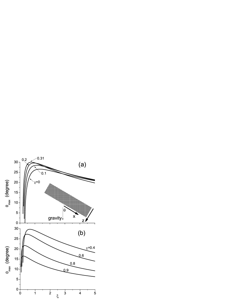
Figure 1: Variation of the maximum angle of inclination with the parameters $\xi$ and $\chi$ calculated with the potential Eq (5) and the strain Eq (13).

with $\tau\equiv u_{xz}/\Delta$, where $\tau^{2}=u_{s}^{2}/\left(2\Delta^{2}\right)-1/3$. Inserting the strain Eq (13) into (69,73), we obtain

$$\sigma_{xz} = -{\frac{2+\chi}{\xi}\Delta}^{3/2}\tau\,,$$ (14)

$$\sigma_{zz} = \frac{9\xi+5\chi+15}{9\xi}{\Delta}^{3/2}+\frac{\chi+2}{2\xi}{\Delta}^{3/2}{\tau}^{2}.$$ (15)

In addition, because of the force balance $\nabla_{j}\sigma_{ij}=\rho g_{i}$, the two stresses are also related by

$$\sigma_{xz}=\sigma_{zz}\tan\theta.$$ (16)

It is worth remarking that if we insert the strain Eq (13) into the Hessian matrix $H_{\alpha\beta}$, we find for $\chi>0$ that two eigenvalues are $4-\chi\left(1\pm 3\,\sqrt{{1}+4\,{\tau}^{2}}\right)$, implying that a stable layer exists only for $\chi<1$, because at least one eigenvalue is negative for $\chi>1$. As the other eigenvalues cannot be expressed analytically, we now consider $\det(H_{\alpha\beta})=0$, finding

$$\det(H_{\alpha\beta})=\frac{4\left(2+\chi\right)}{{\xi}^{6}}{\Delta}^{3}\,D_{1}D_{2},$$ (17)

with

$$D_{1} = {\left(-4+2\,\chi+2\,{\chi}^{2}+9\,{\chi}^{2}{\tau}^{2}\right),}$$ (18)

$$D_{2} = {27\chi^{2}\left(\chi+2\right)\tau^{4}+3\left(-30\chi+12\chi^{2}+5\chi^{3}+36\xi\chi^{2}+12\right)\tau^{2}}$$

$${+2\left(\chi-1\right)\left(4\chi+\chi^{2}-6\right)+36\,\xi\,\left({\chi}^{2}-1\right).}$$

The real roots of $D_{1}=0$ are ${\tau}_{\pm}{=\pm}\sqrt{4-2\chi^{2}-2\chi}{/}3{\chi}$, that of $D_{2}=0$ are

$$\tau_{c} = \,\pm\frac{1}{3{\chi}}\sqrt{{\frac{k_{1}+\sqrt{k_{2}}}{2\left(2+\chi\right)}}},\qquad\text{ \ with}$$ (20)

$$k_{1} = -5\,{\chi}^{3}-12\left(3\xi+1\right)\chi^{2}+30\,\chi-12,$$ (21)

$$k_{2} = \chi^{6}-72\xi\chi^{5}+12\left(108\xi^{2}-5\right)\chi^{4}-24\left(72\xi+11\right)\allowbreak\chi^{3}$$

$$+36\left(48\xi+25\right)\chi^{2}-720\chi+144.$$

(Because $k_{1}<0$ for $\chi\in\left(0,1\right)$, positive square root for $\sqrt{k_{2}}$ ie taken here.) Requiring the vanishing eigenvalue to be the smallest one, we find yield to occur at $\tau=\tau_{c}$, implying a maximum angle of inclination by employing Eqs (14,15),

$$\theta_{\max}=\mp\arctan\,\left[{\frac{18\,\left(2+\chi\right)\tau_{c}}{9\left(\chi+2\right)\tau_{c}^{2}+18\,\xi+30+10\,\chi}}\right].$$ (23)

Inserting $\tau_{c}$ of Eq (20) into it, and remembering that the sign only indicates a left or right inclination, we obtain the absolute value for the maximal angle as

$$\theta_{\max}=\arctan\,\left[{\frac{6\,\sqrt{2}{\chi}\sqrt{2+\chi}\sqrt{{k_{1}+\sqrt{k_{2}}}}}{k_{1}+\sqrt{k_{2}}+36\,\xi{\chi}^{2}+60{\chi}^{2}+20\,\chi^{3}}}\right].$$ (24)

It is nice to have an analytic expression for $\theta_{\max}$, which reduces to the results of JL1 for $\chi\rightarrow 0$ i.e.: $\tau_{c}\rightarrow\sqrt{\xi-1/3}$ and $\theta_{c}\rightarrow\arctan\left[\sqrt{9\xi-3}/\left(3\xi+2\right)\right]$.

In fig.1, the expression of Eq (24) for $\theta_{\max}$ is plotted against $\xi$ for various $0<\chi<1$. The biggest value $\theta_{\max}=30^{\circ}$ is achieved at $\xi\simeq 0.71$ and $\chi\simeq 0.31$. More specifically, as $\chi$ increases from $0$ to $0.31$, the peak of $\theta_{\max}$ versus $\xi$ increases too, but decreases after that.

A final remark: the elastic strain of Eq (13) is a result of assuming that displacement vector $U_{i}$ varies only with the layer depth $z$, and has nonvanishing components along the $x$ and $z$ directions, $U_{y}=0$. Then yield, at $\theta=\theta_{\max}$, occurs simultaneously in the whole layer. This is an idealization. In reality, the displacement vector should also have a nonvanishing $y$ component. Then yield will probably start at the layer top. This case will be studied elsewhere.

III The Yield Surface

In this section, we consider uniform stress $\sigma_{ij}$ and density $\rho$, and employ the coordinate system of the principle directions of the stress. The elastic strain $u_{ij}$ is also uniform and in its principle system, ie, $\sigma_{ij}=0$ and $u_{ij}=0$ for $i\neq j$, see Appendix.

Instead the principle strains $u_{xx}$, $u_{yy}$, $u_{zz}$, we shall, for simplicity, use $\Delta$, $\mathcal{S}\geq 0$ and $L$, where

$$u_{xx} = -\frac{\Delta}{3}\left[1-\mathcal{S}\sin\left(L-\frac{\pi}{3}\right)\right],$$ (25)

$$u_{yy} = -\frac{\Delta}{3}\left(1+\mathcal{S}\sin L\right),$$ (26)

$$u_{zz} = -\frac{\Delta}{3}\left[1-\mathcal{S}\sin\left(L+\frac{\pi}{3}\right)\right].$$ (27)

(In soil mechanics $L$ is usually called as Lode angle, of which value range is taken as $[0,2\pi)$). And we have the following expressions for the principle stresses,

$$\frac{\sigma_{xx}}{{\Delta}^{3/2}} = 3\,\sqrt{3}+{\frac{\mathcal{S}}{4\xi}\left(12\cos L-4\sqrt{3}\sin L+\sqrt{3}\mathcal{S}\right)}$$

$${+}\frac{\chi\mathcal{S}^{2}}{24\xi}\left(6\sqrt{3}\cos 2L-18\sin 2L+\sqrt{3}\mathcal{S}\sin 3L\right),$$

$$\frac{\sigma_{yy}}{{\Delta}^{3/2}} = 3\sqrt{3}\,+\frac{\sqrt{3}}{4\xi}\mathcal{S}\left(\mathcal{S}+8\sin L\right)$$

$$-\frac{\sqrt{3}\chi}{24\xi}\mathcal{S}^{2}\left(12\cos 2L-\mathcal{S}\sin 3L\right),$$

$$\frac{\sigma_{zz}}{{\Delta}^{3/2}} = 3\sqrt{3}\,-\frac{\mathcal{S}}{4\xi}\left(12\cos L+4\sqrt{3}\sin L-\sqrt{3}\mathcal{S}\right)$$

$$+\frac{\chi\mathcal{S}^{2}}{24\xi}\left(18\sin 2L+6\sqrt{3}\cos 2L+\sqrt{3}\mathcal{S}\sin 3L\right).$$

The pressure and the deviatoric stresses $q,Q$ are simpler, with $\Delta$ factored out,

$$P \equiv \sigma_{kk}/3=\frac{\sqrt{3}}{\xi}{\Delta}^{3/2}\left(3\xi\,+\frac{1}{4}\mathcal{S}^{2}+\frac{\chi}{24}\mathcal{S}^{3}\sin 3L\right),$$ (31)

$$q \equiv \sigma_{zz}-\sigma_{xx}=\frac{3}{2\xi}{\Delta}^{3/2}\,\mathcal{S}\left(\chi\mathcal{S}\sin 2L-4\cos L\right),$$ (32)

$$Q/3 \equiv \left(P-\sigma_{yy}\right)=\frac{\sqrt{3}}{2\xi}\Delta^{3/2}\mathcal{S}\left(\chi\mathcal{S}\cos 2L-2\sin L\right).$$ (33)

III.1 The Cylindrically Symmetric Case

For $\sigma_{xx}=\sigma_{yy}$ and $u_{xx}=u_{yy}$, the sample is cylindrically symmetric, implying a Lode angle $L=\pi/6$ or $7\pi/6$, see Eqs.(25,26). Cylindrical symmetry is usually assumed in analyzing the so-called ”triaxial test,” widely used in soil mechanics. Inserting these Lode angles into Eqs (31,32), we obtain

$$\frac{q}{P}=\frac{18\,\mathcal{S}}{\chi\mathcal{S}^{3}+6\mathcal{S}^{2}+72\xi}\times\left\{\begin{array}[]{c}\left(\chi\mathcal{S}-4\right)\\ \left(\chi\mathcal{S}+4\right)\end{array}\right.\text{ \ }\left.\begin{array}[]{l}\text{for }L=\pi/6,\\ \text{for }L=7\pi/6.\end{array}\right.$$ (34)

Note $L=\pi/6$ is the case of triaxial extension with $q<0$, while $L=7\pi/6$ is the case of triaxial compression with $q>0$. At yield, $\mathcal{S=S}_{yield}$, Eq (34) implies $q\sim P$, and in the stress space spanned by $P,q$ yields two straight lines.

To obtain the value for $\mathcal{S}_{yield}$, we calculate the determinant $\det(H_{\alpha\beta})$, obtaining

$$\det(H_{\alpha\beta})=\frac{27{\Delta}^{3}}{16{\xi}^{6}}\,D_{1}^{2}D_{2}^{2}D_{3},$$ (35)

where for $L=\pi/6$:

$$D_{1} = {\chi}\mathcal{S}{+2},$$ (36)

$$D_{2} = {\chi}\mathcal{S}{-4},$$ (37)

$$D_{3} = \chi^{2}\mathcal{S}^{4}-8\chi\mathcal{S}^{3}-24\mathcal{S}^{2}-144\xi\chi\mathcal{S}+288\xi;$$ (38)

and for $L=7\pi/6$:

$$D_{1} = -{\chi}\mathcal{S}{+2},$$ (39)

$$D_{2} = -{\chi}\mathcal{S}{-4},$$ (40)

$$D_{3} = \chi^{2}\mathcal{S}^{4}+8\chi\mathcal{S}^{3}-24\mathcal{S}^{2}+144\xi\chi\mathcal{S}+288\xi.$$ (41)

If $\chi=0$, the equation $\det(H_{\alpha\beta})=0$ reduces to $D_{3}=48\mathcal{S}^{2}-576\xi=0$ for both Lode angles, implying $\mathcal{S}_{yield}=\sqrt{12\xi}$ for extension and compression. Inserting this into Eq (34), we have $q/P=\pm\sqrt{3/\xi}$, the two straight yield lines are then symmetric about the P-axis.

Figure 2: Yield behavior as determined by the energy Eq (5), for the case of cylindrical symmetry. (a) Straight yield line for $\xi=1$ and $\chi=0.2$. (b) Variation of the slope of yield line with $\xi$ for $\chi=0$,0.2,0.4,0.6,0.8,1 (increasing indicated by arrows). (c) The difference between the slopes for compression and extension.

For $\chi\neq 0$, one needs to resort to numerical calculation, which shows that $\mathcal{S}_{yield}\geqslant 0$ is given by the smallest positive root of $D_{3}=0$. Yet because Eqs (38) and (41) are different, $\mathcal{S}_{yield}$ is different for extension and compression, and so are the two slopes, see fig.2-a. This unsymmetric behavior of yield is well documented and familiar in soil mechanics. Within the present framework, it is a measure of how much the third invariant influences granular elasticity. Fig.2-b shows variation of the slope of yield line with the parameter $\xi$, at varying $0\leqslant\chi<1$. In agreement with the observations, the absolute value of the slopes is always greater for compression than that for extension, see fig.2-c.

III.2 The General Case

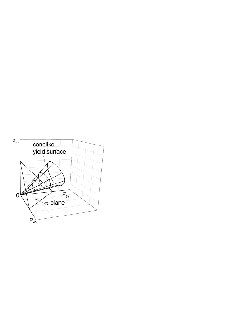
Figure 3: Yield surface, $\pi$-plane and their intersection loci in principle-stress space. The $\pi$-plane is defined by constant $\sigma_{xx}+\sigma_{yy}+\sigma_{zz}$.

Next we consider the general case, with $\sigma_{xx}\neq\sigma_{yy}\neq\sigma_{zz}$. Inserting the expressions (25,26,27) into the Hessian matrix, and calculating its determinant, we have

$$\det(H_{\alpha\beta})=\frac{27\Delta^{3}}{16\xi^{6}}D_{1}D_{2},$$ (42)

where

$$D_{1} = \chi^{3}\mathcal{S}^{3}\sin 3L-6\,{\chi}^{2}{\mathcal{S}}^{2}+32,$$ (43)

$$D_{2} = \chi^{3}\mathcal{S}^{5}\sin 3L-6\,{\chi}^{2}{\mathcal{S}}^{4}-40\chi\mathcal{S}^{3}\sin 3L$$

$$-48\left(3\xi\chi^{2}+1\right)\mathcal{S}^{2}+576\,\xi.$$

It can be demonstrated numerically that for any $L\in\left[0,2\pi\right)$, yield $\mathcal{S}=\mathcal{S}_{yield}$ is given by the smallest positive root of $D_{1,2}=0$, which is also computed numerically. Inserting the yield strain $\left(L,\mathcal{S}_{yield}\right)$ into (III,III,III) the yield surface in the stress space can be plotted. Since the compressional strain $\Delta$ is an overall factor, the surface is conelike, as illustrated in fig.4. We present the yield surface (as is customary in soil mechanics) with a closed curve given by its intersection with the so called $\pi$-plane, defined by $P=$const., see fig.3. For the conelike surface it is convenient to introduce the rectangular coordinates in the $\pi$-plane defined by

$$\pi_{1} = \left(\sigma_{zz}-\sigma_{yy}\right)/\sqrt{2}P,$$ (45)

$$\pi_{2} = \left(2\sigma_{xx}-\sigma_{yy}-\sigma_{zz}\right)/\sqrt{6}P.$$ (46)

Using Eqs (III,III,III), they become

$$\pi_{1} = \frac{6\sqrt{6}\mathcal{S}\left(\mathcal{S}\chi\sin 2L-4\cos L\right)}{\chi\left(\sin 3L\right)\mathcal{S}^{3}+6\mathcal{S}^{2}+72\xi},$$ (47)

$$\pi_{2} = \sqrt{\frac{3}{2}}\frac{6\mathcal{S}^{2}\chi\cos 2L-24\mathcal{S}\sin L+24\sqrt{3}\mathcal{S}\cos L-6\sqrt{3}\allowbreak\mathcal{S}^{2}\chi\sin 2L}{\chi\left(\sin 3L\right)\mathcal{S}^{3}+6\mathcal{S}^{2}+72\xi}.$$ (48)

Inserting $\left(L,\mathcal{S}_{yield}\right)$ into them the yield curve in the $\pi$-plane can be plotted, see fig.4. On the other hand, the yield surfaces of the Coulomb, Drucker-Prager, Lade-Duncan and Matsuoka-Nakai models, also conelike, and their loci in the $\pi$-plane, may be plotted directly – using Eqs (6,7,8,9) and Eqs (45,46) – and compared.

The Drucker-Prager yield model can be reproduced exactly by the energy Eq (5) with $\chi=0$. It is a circle in the $\pi$-plane, see fig.4-a. As $\chi$ increases from 0, the yield curve of Eq (5) is distorted from a circle to a triangle-like curve, in fairly good agreement with the Lade-Duncan and Matsuoka-Nakai models, see fig.4-b,c. Although the Coulomb model is a hexagon, with three more corners, see the dotted line of fig.4-b, the difference seems insignificant.

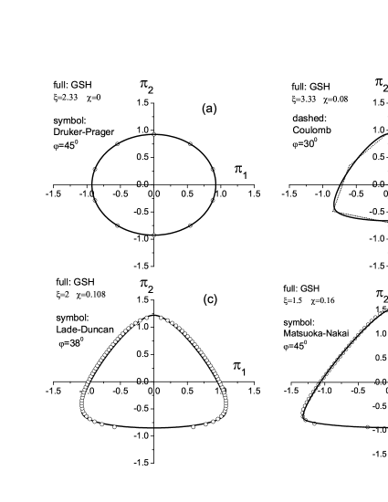
Figure 4: Yield loci in the $\pi$-plane calculated with the energy Eq (5), in comparison with various yield models, from (a) to (d): Drucker-Prager, Coulomb, Lade-Duncan, Matsuoka-Nakai.

We note the large difference between the maximum angle of inclination $\theta_{\max}$ and the friction angle $\varphi$. Employing the parameters of Fig.6 below: $\xi=1$, $\chi=0.25$, we obtain $\theta_{\max}=29.8^{\circ}$, and $\varphi=65^{\circ},54^{\circ},60^{\circ}$ for the Coulomb, Lade-Duncan, and Matsuoka-Nakai model, respectively.

IV The Compliance Tensor

Since GSH is a unified description of granular behavior, the energy of Eq (5) is expected to also account for the elastic stiffness and the speed of elastic waves, both experimentally accessible. The stiffness tensor $M_{ijmn}$ is of fourth order and defined as

$$\delta\sigma_{ij}\equiv M_{ijmn}\delta u_{mn}=-(\partial^{2}w/\partial u_{ij}\partial u_{mn})\delta u_{mn},$$ (49)

while the compliance tensor is its inverse,

$$du_{ij}=\lambda_{ijmn}d\sigma_{mn}.$$ (50)

The differential forms of Eqs (49,50) are also referred to as incremental stress-strain relation in soil mechanics. Physically, the components of the stiffness tensor can be interpreted as response coefficients of a small stress change to a strain increment, or vice versa for those of the compliance tensor.

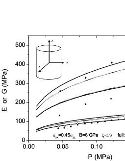
Figure 5: Comparison of compliance coefficients between those measured in Kuwano and calculated via Eq (49).

Systematic measurements of the response coefficients as functions of stress and density was carried out by Kuwano and Jardine for the case of cylindrical symmetry using a triaxial apparatus Kuwano . A comparison of their data with the GSH calculation obtained for $\chi=0$ was given in JL2 ; SoilMech . Here we consider whether the agreement may be further improved by a finite $\chi$. In fig.5, we plotted the four compliance components, denoted as $E_{xx}\equiv-1/\lambda_{xxxx}$, $E_{zz}\equiv-1/\lambda_{zzzz}$, $G_{xz}\equiv-1/4\lambda_{xzxz}$ and $G_{xy}\equiv-1/4\lambda_{xyxy}$, as functions of $P$. The agreement is clearly improved for $\chi=0.1$. Especially noteworthy is the fact that $G_{xz}$ and $G_{xy}$ degenerate for $\chi=0$, but are split appropriately, in the correct order, for $\chi=0.1$, again indicating that the sign of $\chi$ is positive.

V Elastic Waves

A further important elastic property is the speed $c_{i}$ of elastic waves, which can be calculated from the square root of the appropriate eigenvalues of the acoustic tensor, see ge4 ; LL6 ,

$$C_{ij}=\frac{k_{m}k_{n}}{\rho k^{2}}\frac{\partial^{2}w}{\partial u_{im}\partial u_{nj}}$$ (51)

where $k_{m}$ is the wave vector of propagation, with $k^{2}\equiv k_{m}k_{m}$. Inserting the energy of Eq (5) into (51), and eliminating the strain with the help of Eq (1), we can obtain different velocities as functions of the stress: $c_{i}=c_{i}\left(\sigma_{ij}\right)$. Such a calculation with $\chi=0$ has been given in ge4 , resulting in satisfactory agreement, though the weak variation of the transverse wave velocity with varying polarization and direction of propagation was not reproduced. Here, we focus on this and the additional difference taking $\chi\neq 0$. Since the energy is a homogenous function of the strain, or equivalently the stress, the stress dependence of the velocities can be factorized as $c_{i}\sim P^{1/6}f\left(k_{m},\xi,\chi,\sigma_{ij}^{\ast}/P\right)$, where the factor $f\sim c_{i}/P^{1/6}$ represents the influences of shear stresses on sound speeds (from which the values of the parameters $\xi,\chi$ may be obtained with great accuracy). Fig. 6 shows the calculated $c_{i}/P^{1/6}$, setting $\xi=1$ and $\chi=0.25$, in comparison with the data reported in jia . Cylindrical symmetry is assumed, and the wave is taken to propagate along axial (Fig. 6-a) and radial directions (Fig. 6-b). Then $c_{i}/P^{1/6}$ depends only on $q/P$, or equivalently on $q/\sigma_{xx}=3(q/P)(3-q/P)^{-1}$. Clearly, GSH reproduces the data fairly well, where especially the order of splitting of the transverse waves velocity, when either polarized along the axial or the radial direction is correct, once again indicating that $\chi>0$.

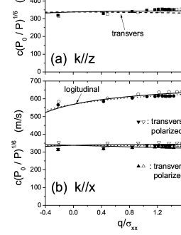
Figure 6: Comparison of sound speeds as calculated employing the energy expression of Eq (5) with the measurements reported in jia . $P_{0}$ is the atmosphere pressure.

Finally, we note that irrespective of the energy expression, there can only be two different transverse velocities in a cylindrical geometry along the principle axes. Therefore, if hardened experimental evidences to the contrary arises, this would indeed be a reason to include an additional variable such as the intrinsic anisotropy.

Assuming a general expression for the energy, $d\tilde{w}=\dots d\Delta+\dots du_{s}+\dots du_{t}$, with $d\Delta=-\delta_{ij}du_{ij}$, $du_{s}=u_{ij}^{0}du_{ij}/{u_{s}}$, $du_{t}=u_{im}u_{mj}/{u_{t}^{2}}$, we calculate the stress as

$${\sigma}_{ij}=\tilde{f}_{1}(\Delta,u_{s},u_{t})\delta_{ij}+\tilde{f}_{2}(\Delta,u_{s},u_{t})u_{ij}+\tilde{f}_{3}(\Delta,u_{s},u_{t})u_{im}u_{mj},$$ (52)

where $\tilde{f}_{i}$ depend on the energy $\tilde{w}$. Similarly, the stiffness tensor $\tilde{M}_{ijkl}$ is generally given as

$$\tilde{M}_{ijkl}=g_{1}\delta_{ij}\delta_{kl}+g_{2}\left(u_{ij}\delta_{kl}+u_{kl}\delta_{ij}\right)+g_{3}\left(u_{im}u_{mj}\delta_{kl}+u_{km}u_{ml}\delta_{ij}\right)\\ +g_{4}\left(\delta_{ik}\delta_{jl}+\delta_{il}\delta_{jk}\right)+g_{5}u_{ij}u_{kl}+g_{6}\left(u_{ij}u_{km}u_{ml}+u_{kl}u_{im}u_{mj}\right)\\ +g_{7}u_{im}u_{mj}u_{km}u_{ml}+g_{8}\left(u_{ki}\delta_{lj}+u_{kj}\delta_{li}+u_{li}\delta_{jk}+u_{lj}\delta_{ik}\right)$$ (53)

with $g_{i}=g_{i}(\Delta,u_{s},u_{t})$ again to be calculated from $\tilde{w}$. In the system of principle axes, $u_{ij}=u_{(i)}\delta_{ij}$, the stiffness tensor reads

$$\tilde{M}_{ijkl} = \Bigl{[}g_{1}+g_{2}\left(u_{(i)}+u_{(k)}\right)+g_{5}u_{(i)}u_{(k)}+g_{3}\left(u_{(i)}^{2}+u_{(k)}^{2}\right)$$ (54)

$$+g_{6}\left(u_{(k)}^{2}u_{(i)}+u_{(i)}^{2}u_{(k)}\right)\delta_{ij}+g_{7}u_{(i)}^{2}u_{(k)}^{2}\Bigr{]}\delta_{ij}\delta_{kl}$$

$$\Bigl{[}g_{4}+g_{8}\left(u_{(i)}+u_{(j)}\right)\Bigr{]}\left(\delta_{ik}\delta_{jl}+\delta_{il}\delta_{jk}\right)$$

$$:= g(i,k)\delta_{ij}\delta_{kl}+h(i,j)\left(\delta_{ik}\delta_{jl}+\delta_{il}\delta_{jk}\right).$$

The acoustic tensor $\tilde{C}_{il}\sim\tilde{M}_{ijkl}n_{j}n_{k}$ (with $n_{i}\equiv k_{i}/|k|$) therefore is

$$\tilde{C}_{il} \sim \left(g(i,l)+h(i,l)\right)n_{i}n_{l}$$

$$+\left(g_{4}+g_{8}\left(u_{(i)}+\left[u_{2}+\left(u_{1}-u_{2}\right)n_{1}^{2}+\left(u_{3}-u_{2}\right)n_{3}^{2}\right]\right)\right)\delta_{il}$$

$$= H(i,l)n_{i}n_{l}+\left(g_{4}+g_{8}\left(u_{(i)}+u_{dev}\right)\right)\delta_{il},$$

with $H(i,l)=g(i,l)+h(i,l)$ and $u_{dev}(\vec{n})=u_{2}+\left(u_{1}-u_{2}\right)n_{1}^{2}+\left(u_{3}-u_{2}\right)n_{3}^{2}$.

For cylindrical symmetry, denoting z as the preferred direction, $u_{1}=u_{2}\neq u_{3}$, we have $H(1,1)=H(2,2)=H(1,2)$ and $u_{dev}=u_{1}+\left(u_{3}-u_{1}\right)n_{3}^{2}$. We have, if the wave vector is along z ($n_{3}=1$, $n_{1}=n_{2}=0$),

$$\tilde{C}_{z} = \left(\begin{array}[]{ccc}g_{4}+g_{8}\left(u_{1}+u_{3}\right)&0&0\\ 0&g_{4}+g_{8}\left(u_{1}+u_{3}\right)&0\\ 0&0&H_{33}+g_{4}+2g_{8}u_{3}\end{array}\right);\quad$$ (58)

if it is along x ($n_{1}=1$, $n_{2}=n_{3}=0$),

$$\tilde{C}_{x} = \left(\begin{array}[]{ccc}H_{11}+g_{4}+2g_{8}u_{1}&0&0\\ 0&g_{4}+2g_{8}u_{1}&0\\ 0&0&g_{4}+g_{8}\left(u_{3}+u_{1}\right)\end{array}\right);$$ (62)

if it is along y ($n_{2}=1$, $n_{1}=n_{3}=0$),

$$\tilde{C}_{y} = \left(\begin{array}[]{ccc}g_{4}+2g_{8}u_{1}&0&0\\ 0&H_{11}+g_{4}+2g_{8}u_{1}&0\\ 0&0&g_{4}+g_{8}\left(u_{3}+u_{1}\right)\end{array}\right).$$ (66)

We note two different eigenvalues of the acoustic tensor for the transverse case,

$$\tilde{C}_{z,11}=\tilde{C}_{z,22}=\tilde{C}_{x,33}=\tilde{C}_{y,33}\neq\tilde{C}_{x,22}=\tilde{C}_{y,11},$$ (67)

and realize that there can only be two different velocities. Note also that without $g_{8}$ that stems from the third invariant, only one transverse velocitiy exists.

VI Discussion and Conclusions

Macroscopically speaking, granular media at rest are elastic, and one can account for all its static, mechanic behavior including yield, compliance coefficients, and sound propagation by a single potential, the elastic energy. Finding an quantitatively appropriate potential is certainly interesting and useful, and the expression given in Eq  (5) seems a good starting point. It is a generalization of the potential given in granR1 ; JL1 , with a term depending on the cubic strain invariant. All empirical yield models and the other experiments considered above support this term. As mentioned in the introduction, yield models in soil mechanics are usually selected by personal experience, preference or convenience, and there seems no consensus which one is best. The uncertainty of the situation may be reduced with the help of the considered potential, as it unifies these models, and link them to other easily measurable elastic properties such as sound speeds, and compliance tensor. In this context, we would like to stress the importance of more accurate and systematic experiments, such as simultaneous measurement of sound velocity and yield.

It is important to realize that yield as considered here happens at the highest possible stress at which the system may maintain an elastic, static solution. It is different from that obtained under stead shear: When approaching the critical state from an isotropic one, the approach is not monotonous if the starting density is high, and the limiting, so-called critical stress is lower than some of the stress values the system has undergone. At all these stress states, if the strain rate is stopped, the system will stop as well and retain its stress statically. Therefore, it is still below yield at all these stress states. Measurements carried out with steady shearing samples therefore do not reveal the yield surface. Interpreting the results as such will lead to discrepancies.

Moreover, density also influences elastic properties of granular materials, which was considered in granR2 , but is neglected here for simplicity. In granR2 , we have shown how to include the density dependence of the energy $w$ to account for the so-called “cap” cs , or the sound velocity as measured by Hardin and Richart HR . These features are easily transferred to the energy of Eq (5). Summarizing, we believe that although the details of granular elasticity is complicated, and more accurate experiments are needed for further clarification, Eq (5) provides a reasonable start point.

Appendix A Stress-Strain Relation

From the energy of Eq (5), we may calculate the stress as a function of the elastic strain via $\sigma_{ij}=-\partial w/\partial u_{ij}$, obtaining

$$\sigma_{xy} ={\frac{3\chi\left(u_{xz}u_{yz}-u_{xy}u_{zz}\right)-\left(\chi+2\right)\Delta u_{xy}}{\sqrt{\Delta}\xi},}$$ (68)

$$\sigma_{xz} ={\frac{3\chi\left(u_{xy}u_{yz}-u_{xz}u_{yy}\right)-\left(\chi+2\right)\Delta u_{xz}}{\sqrt{\Delta}\xi},}$$ (69)

$$\sigma_{yz} ={\frac{3\chi\left(u_{xy}u_{xz}-u_{yz}u_{xx}\right)-\left(\chi+2\right)\Delta u_{yz}}{\sqrt{\Delta}\xi},}$$ (70)

and

$$q \equiv\sigma_{zz}-\sigma_{xx}={\frac{1-\chi}{\xi/2}\sqrt{\Delta}\left(u_{xx}-u_{zz}\right)+\frac{3\chi}{\xi}}\frac{u_{yz}^{2}-u_{xy}^{2}-u_{xx}^{2}+u_{zz}^{2}}{\sqrt{\Delta}},$$ (71)

$$\widetilde{q} \equiv\sigma_{yy}-\sigma_{xx}={\allowbreak\frac{1-\chi}{\xi/2}\sqrt{\Delta}\left(u_{xx}-u_{yy}\right)+}\frac{\allowbreak 3\chi}{\xi}\frac{u_{yz}^{2}-u_{xz}^{2}-u_{xx}^{2}+u_{yy}^{2}}{\sqrt{\Delta}}.$$ (72)

$$\sigma_{zz} =\frac{9\xi+5\chi+15\allowbreak}{9\xi}{\Delta}^{3/2}+\frac{3\left(\chi+2\right)\allowbreak}{2\xi}\sqrt{\Delta}\left(u_{xx}+u_{yy}\right)$$ (73)

$$+\frac{1}{\sqrt{\Delta}\xi}\left(u_{xx}^{2}+u_{xx}u_{yy}+u_{yy}^{2}+u_{xy}^{2}+u_{xz}^{2}+u_{yz}^{2}\right)$$

$$+\frac{\chi}{2\xi\sqrt{\Delta}}\left(u_{xx}^{2}+4u_{xx}u_{yy}+u_{yy}^{2}-2u_{xy}^{2}+u_{xz}^{2}+u_{yz}^{2}\right)$$

$$+\frac{3\chi}{2{\Delta}^{3/2}\xi}\left[\left(u_{xy}^{2}-u_{xx}u_{yy}\right)\left(u_{yy}+u_{xx}\right)-u_{xz}^{2}u_{yy}-u_{yz}^{2}u_{xx}+2u_{xy}u_{xz}u_{yz}\right]$$

Clearly, if the strain is diagonal, the stress is too. In the principle coordinate, the stress-strain relations becomes

$$q ={\frac{1-\chi}{\xi/2}\sqrt{\Delta}\left(u_{xx}-u_{zz}\right)+\frac{3\chi}{\xi}}\frac{-u_{xx}^{2}+u_{zz}^{2}}{\sqrt{\Delta}},$$ (74)

$$\widetilde{q} ={\allowbreak\frac{1-\chi}{\xi/2}\sqrt{\Delta}\left(u_{xx}-u_{yy}\right)+}\frac{\allowbreak 3\chi}{\xi}\frac{-u_{xx}^{2}+u_{yy}^{2}}{\sqrt{\Delta}}.$$ (75)

and

$$\sigma_{zz} =\frac{9\xi+5\chi+15\allowbreak}{9\xi}{\Delta}^{3/2}+\frac{3\left(\chi+2\right)\allowbreak}{2\xi}\sqrt{\Delta}\left(u_{xx}+u_{yy}\right)$$ (76)

$$+\frac{1}{\sqrt{\Delta}\xi}\left(u_{xx}^{2}+u_{xx}u_{yy}+u_{yy}^{2}\right)$$

$$+\frac{\chi}{2\xi\sqrt{\Delta}}\left(u_{xx}^{2}+4u_{xx}u_{yy}+u_{yy}^{2}\right)$$

$$+\frac{3\chi}{2{\Delta}^{3/2}\xi}\left[\left(-u_{xx}u_{yy}\right)\left(u_{yy}+u_{xx}\right)\right]$$

- (1) Y.M. Jiang and M. Liu, Granular Matter, 11, 139 (2009); Y.M. Jiang and M. Liu, Mechanics of Natural Solids, edited by D. KolymbasandG. Viggiani, Springer, pp. 27–46 (2009); G. Gudehus, Y.M. Jiang, and M. Liu, Granular Matter, 1304, 319 (2011).
- (2) D.O. Krimer, M. Pfitzner, K. Bräuer, Y. Jiang, M. Liu, Granular Elasticity: General Considerations and the Stress Dip in Sand Piles, Phys. Rev. E74, 061310 (2006).
- (3) K. Bräuer, M. Pfitzner, D.O. Krimer, M. Mayer, Y. Jiang, M. Liu, Granular Elasticity: Stress Distributions in Silos and under Point Loads, Phys. Rev. E74, 061311 (2006);
- (4) Y.M. Jiang, M. Liu, A Brief Review of “Granular Elasticity”, Eur. Phys. J. E 22, 255 (2007).
- (5) Y.M. Jiang, M. Liu, Incremental stress-strain relation from granular elasticity: Comparison to experiments, Phys. Rev. E 77, 021306 (2008).
- (6) Y.M. Jiang, M. Liu, Energy Instability Unjams Sand and Suspension, Phys. Rev. Lett. 93, 148001(2004).
- (7) M. Mayer and M. Liu, Phys. Rev. E 82, 042301 (2010).
- (8) Y.M. Jiang, M. Liu, From Elasticity to Hypoplasticity: Dynamics of Granular Solids, Phys. Rev. Lett. 99, 105501 (2007).
- (9) S. Mahle, Y. Jiang, and M. Liu, arXiv:1006.5131v3[physics.geo-ph] (2010).
- (10) Stefan Mahle, Yimin Jiang, M. Liu, arXiv:1010.5350v1 [cond-mat.soft] (2010).
- (11) Y.M. Jiang, M. Liu, Granular Elasticity without the Coulomb Condition, Phys. Rev. Lett. 91, 144301 (2003).
- (12) Y. Khidas and X.P. Jia, Phys. Rev. E, 81, 021303 (2010).
- (13) R. Kuwano and R. J. Jardine, Géotechnique 52, 727 2002.
- (14) P.W. Humrickhouse, J.P. Sharpe,1 and M.L. Corradini, Comparison of hyperelastic models for granular materials, Phys.Rev. E 81, 011303 (2010)
- (15) C.A. Coulomb, Mem. de Math. de l’Acad. Royale des Science 7, (1776) 343.
- (16) R.M. Nedderman, Statics and Kinematics of Granular Materials, Cambridge university press, Cambridge (1992).
- (17) D.C. Drucker and W Prager, Soil mechanics and plastic analysis for limit design. Quarterly of Applied Mathematics, 10(2), 157 (1952).
- (18) P.V. Lade and J.M. Duncan, Cubic triaxial tests on cohensionless soil, Proc. ASCE, JSMFD, vol 99, No SM10, 1973; P.V. Lade and J.M. Duncan, Elastoplastic Stress-Strain Theory for Cohensionless Soil, Proc. ASCE, JGTD, vol 101, No GT10 (1975).
- (19) H. Matsuoka, On the significance of the spatial mobilized plane. Soils & Foundations. 1976 6(1): 91-100; H. Matsuoka and T. Nakai, Stress-Strain relationship of soil based on the SMP. Proc. 9th ICSMFE, specialty session 9, 153-163 (1977).
- (20) L.D. Landau and E.M. Lifshitz, Theory of Elasticity (New York, Pergamon Press, 3rd edn. 1986)
- (21) A. Schofield and P. Wroth, Critical State Soil Mechanics. McGraw-Hill, London (1968)
- (22) B.O. Hardin, F.E. Richart, Elastic wave velocities in granular soils. J. Soil Mech. Found. Div. ASCE 89(SM1), 33–65 (1963)