Modeling two-language competition dynamics

Abstract

During the last decade, much attention has been paid to language competition in the complex systems community, that is, how the fractions of speakers of several competing languages evolve in time. In this paper we review recent advances in this direction and focus on three aspects. First we consider the shift from two-state models to three state models that include the possibility of bilingual individuals. The understanding of the role played by bilingualism is essential in sociolinguistics. In particular, the question addressed is whether bilingualism facilitates the coexistence of languages. Second, we will analyze the effect of social interaction networks and physical barriers. Finally, we will show how to analyze the issue of bilingualism from a game theoretical perspective.

I Introduction

The modeling of language dynamics in the general framework of complex systems has been addressed from at least three different perspectives: language evolution (or how the structure of language evolves) Steels (2011), language cognition (or the way in which the human brain processes linguistic knowledge) Edelman and Waterfall (2007), and language competition (or the dynamics of language use in multilingual communities) Solé et al. (2010); Stauffer and Schulze (2005); Wichmann (2008). The latter is the approach followed in this paper in which, therefore, we focus on problems of social interactions. Thus, there is a direct connection with social sciences and social dynamics, since linguistic features represent cultural traits of a specific nature, whose propagation and evolution can in principle be modeled through a dynamics analogous to that of cultural spreading and opinion dynamics Castellano et al. (2009); San Miguel et al. (2005). Furthermore, language dynamics offers the possibility to understand the mechanisms regulating the size evolution of linguistic communities, an important knowledge in the design of appropriate linguistic policies.

This paper reviews recent work on language competition dynamics focusing on models describing interaction in social communities with two languages or two linguistic features ‘‘A’’ and ‘‘B’’. In particular, we consider the special role of bilingual speakers. The emphasis is on two- or three-state models, in the physics jargon, or models with two excluding or non-excluding options, to say it from the perspective of economics and social norms. Languages or linguistic features are considered here as fixed cultural traits in the society, while the more general dynamics of evolving interacting languages is not considered.

We discuss work done in several parallel directions and from different methodological points of view. A first approach reviewed below is the family of competition models, referred to also as ‘‘ecological models of language’’. They can be studied at a macroscopic or mesoscopic level, introducing population densities for the respective language communities or using microscopic agent-based models, where the detailed interactions between agents are taken into account. The formulation can be made at different levels of detail, possibly introducing the effect of population dynamics, geography, and intrinsic or external random fluctuations. A different approach considered is that of game-theoretical models, which allows the description of agents making choices about the language to be spoken at each encounter when limited information is available to them. While in the ecological models each language is initially spoken by a fraction of the population, in the game-theoretical framework we consider the present situation in many societies in which one language is spoken by everyone, while a minority language is only spoken by a proportion of the population. The only relevant dynamics is then the one of the bilingual minority.

The outline of the paper is as follows: Section 2 describes language competition models. A first part is devoted to review the seminal model of Abrams and Strogatz Abrams and Strogatz (2003) and variations thereof, while a second part reviews several models proposed to take into account bilingual agents in this context. Section 3 discusses how to account for geographic effects in the models of language competition dynamics. Section 4 introduces a game-theory perspective into the problem. Section 5 contains some general conclusions and outlook.

II Language competition models

II.1 The Abrams & Strogatz model

The Abrams & Strogatz model (from now on, AS model) Abrams and Strogatz (2003) is the seminal work which triggered a coherent effort from a statistical physics and complex systems approach to the problem of language competition . It is a simple two-state model with two parameters (with a main focus on prestige of the languages ), which the authors fit to real aggregated data of endangered languages such as Quechua (in competition with Spanish), Scottish Gaelic and Welsh (both in competition with English). The original model is a population dynamics model. However in this review, we first introduce its microscopic version Stauffer et al. (2007) and we consider later its population dynamics (mean-field) approximation.

The microscopic or individual based version of the AS model Stauffer et al. (2007) is a two-state model proposed for the competition between two languages in which an agent i sits in a node within a network of $N$ individuals and has $k_{i}$ neighbors. Neighbors are here understood as agents sitting in nodes directly connected by a link. The agent can be in the following states: A, agent using language A (monolingual A); or B, agent using language B (monolingual B). At each iteration we choose one agent i at random and we compute the local densities for each of the states in the neighborhood of node i, $\sigma_{i,l}$ (l=$A$, $B$). The agent changes its state according to the following transition probabilities:

$$p_{i,A\rightarrow B}=(1-s)(\sigma_{i,B})^{a} \quad\quad p_{i,B\rightarrow A}=s(\sigma_{i,A})^{a}\hskip 2.84544pt$$ , (1)

Equations (1) give the probabilities for an agent i to change from state A to B, or vice-versa. These probabilities depend on the local densities ($\sigma_{i,A}$, $\sigma_{i,B}$) and on two free parameters: the prestige of language A, $0\leq s\leq 1$ (the one of language B is $1-s$); and the volatility parameter, $a\geq 0$. Prestige is modeled as a scalar which aggregates multiple factors. In this way, $s$ gives a measure of the different status between the two languages, that is, which is the language that gives an agent more possibilities in the social and personal spheres. Mathematically, it is a symmetry breaking parameter. The case of socially equivalent languages corresponds to $s=0.5$. On the other hand, the volatility parameter gives shape to the functional form of the transition probabilities. The case $a=1$ is the neutral situation, where the transition probabilities depend linearly on the local densities. A high volatility regime exists for $a<1$, where the probability of changing language state is larger than the neutral case, and therefore agents change its state rather frequently. A low volatility regime exists for $a>1$ with a probability of changing language state below the neutral case, and thus agents have a larger resistance to change its state. In this way, the volatility parameter gives a measure of the propensity (or resistance) of the agents to change their language use.

II.1.1 Mean-field approximation

In the limit of infinite population and fully connected society, that is, each agent can interact with any other agent in the population, the model can be described by differential equations for the population densities of agents Abrams and Strogatz (2003),

$$\dot{x}_{A}\! = \!{s_{A}}\,x_{A}^{a}\,x_{B}-{s_{B}}\,x_{B}^{a}\,x_{A}\ ,$$

$$\dot{x}_{B}\! = \!-{s_{A}}\,x_{A}^{a}\,x_{B}+{s_{B}}\,x_{B}^{a}\,x_{A}\ .$$ (2)

Here $x_{i}(t)$, $i=A,B$, represents the fraction of speakers of language $i$ while $s_{i}$ represents the prestige. Using the condition $x_{A}(t)+x_{B}(t)=1$ and following the normalization $s_{A}\!+\!s_{B}\!=\!1$ ($s_{A}=s$), they can be reformulated as a two-parameter single-variable problem for the variable $x_{A}(t)$:

$$\dot{x}_{A}=s_{A}\,x_{A}^{a}\,(1-x_{A})-s_{B}\,(1-x_{A})^{a}\,x_{A}~{}.$$ (3)

The final state reached by the dynamics depends on the initial populations $x_{i}(t_{0})$ and the values of the parameters $s_{i}$ and $a$. Note that from an ecological point of view the reaction term $R(x_{A},x_{B})={s_{A}}x_{A}^{a}x_{B}-{s_{B}}x_{B}^{a}x_{A}$ implies that languages A and B act to each other as preys and predators at the same time Murray (2002), a situation peculiar in ecology but realistic in the competition between cultural traits Abrams and Strogatz (2003).

Abrams and Strogatz found an exponent $a=1.31$ when fitting to real data from the competition between Quechua-Spanish, Scottish Gaelic-English and Welsh-English Abrams and Strogatz (2003). Moreover, they also inferred the corresponding value of $s$ in each of the linguistic situations. The general analysis of the role of parameters $s$ and $a$ in the model is discussed below.

An alternative macroscopic description of the AS model can be obtained defining a magnetization $m=x_{A}-x_{B}=2x_{A}-1$ and a bias parameter $v=1-2s$. The time evolution of the magnetization is given by

$$\frac{dm(t)}{dt}=2^{-(a+1)}(1-m^{2})\left[(1+v)(1+m)^{a-1}-(1-v)(1-m)^{a-1}\right].$$ (4)

Equation (4) describes the evolution of a very large system ($N\gg 1$) at the macroscopic level, neglecting finite size fluctuations. It has the three stationary solutions

$$m_{-}=-x_{B}=-1,~{}~{}~{}m^{*}=\frac{(1-v)^{\frac{1}{a-1}}-(1+v)^{\frac{1}{a-1}}}{(1-v)^{\frac{1}{a-1}}+(1+v)^{\frac{1}{a-1}}}~{}~{}~{}\mbox{and}~{}~{}~{}m_{+}=x_{A}=1.$$ (5)

Solutions $m_{\pm}$ correspond to the dominance of one of the languages, so that a social consensus on which language to be used has been reached. Solution $m^{*}$ corresponds to a situation of coexistence of the two languages. When $a<1$ (large volatility), both solutions $m_{\pm}$ are unstable, and $m^{*}$ is stable, whereas for $a>1$ (small volatility) the opposite happens. In the line $a=1$, $m_{+}$ is unstable (stable) for $v<0$ ($v>0$), and vice-versa for $m_{-}$. Therefore, a structural transition is found at the critical value $a=1$. In Fig. 1, we show the regions of stability and instability of the stationary solutions on the $(a,v)$ plane obtained from the above analysis. We observe a region of coexistence ($m^{*}$ stable) and one of bistable dominance of any of the languages ($m_{+}$ and $m_{-}$ stable) for any value of the prestige parameter.

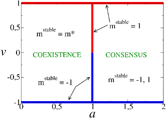
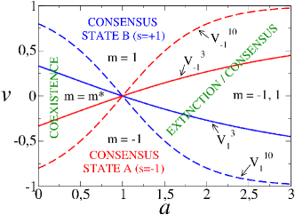
Figure 1: Stability diagram for the AS model in a fully connected network (left) and a degree-regular random networks (right). Solid and dashed lines correspond to degree-regular random networks with degrees $\langle k\rangle=3$ and $\langle k\rangle=10$ respectively. See the text for the definition of the regions. From Ref. Vazquez et al. (2010).

The AS model has been studied within the context of viability theory and resilience Aubin (1991); Chapel et al. (2010). In this framework, it is assumed that the prestige $s$ of the model can be changed in real time by action policies in order to maintain the coexistence of two competing languages, that is, keeping language coexistence viable. In Ref. Chapel et al. (2010) such policies are obtained, studying the effect of varying the volatility parameter. In general, large values of $a$ (small volatility) reduce the set of viable situations for language coexistence.

II.1.2 Random networks

In order to account for local effects in which each agent only interacts with a small fraction of the population one needs to go beyond the mean field approximation. A first step in this direction is considering the AS model in random networks. For these networks a pair approximation can be used in which the state of an agent only depends on the state of its first neighbors. This approximation works well in networks with no correlations to second neighbors. For a degree-regular random network, that is, a network in which each node is randomly connected to a fixed number of $\langle k\rangle$ neighbors, the phase diagram obtained in Ref. Vazquez et al. (2010) is shown in Fig. 1. Compared to the fully connected case, the region of coexistence is found to shrink for $v\neq 0$, as there appear two regions where only the solution corresponding to dominance of the most prestigious language is stable (labeled as CONSENSUS STATE A [B]). These regions become larger, the smaller the average number of neighbors $\langle k\rangle$, because the local effects become more important (see transition lines for $\langle k\rangle=3$ and $\langle k\rangle=10$ in Fig. 1), reducing further the set of parameters for which coexistence is possible.

These regions become larger as local effects in the network become more important as the number of neighbors $\langle k\rangle$ diminish (see transition lines for $\langle k\rangle=3$ and $\langle k\rangle=10$ in Fig. 1), reducing further the set of parameters for which coexistence is possible. The fourth region (EXTINCTION/CONSENSUS) corresponds to situations where dominance in any of the two languages is stable.

II.1.3 Two-dimensional lattices

When two-dimensional lattices are considered, correlations to second neighbors become important. Thus a pair approximation is not enough to describe the system macroscopically. Instead, a field approximation is needed Vazquez and López (2008), which describes well the macroscopic evolution of the system and is able to characterize the different dynamics of the growth of linguistic domains depending on the volatility parameter, $a$. The stability diagram obtained for a square lattice is qualitatively similar to the one found in random networks (Fig. 1), but the region for coexistence is found to be much narrower than the ones observed in complex networks with low degree (small number of neighbors).

In the field approximation Vazquez et al. (2010), we define $\phi_{\bf r}(t)$ as the average magnetization field at site ${\bf r}$ at time $t$, which is a continuous representation of the magnetization at that site ($-1<\phi<1$). In this description, an alternative and more visual way of studying stability is by writing the time evolution of the magnetization field $\phi_{\bf r}$ in the form of a time-dependent Ginzburg-Landau equation

$$\frac{\partial\phi_{\bf r}(t)}{\partial t}=D(\phi_{\bf r})\Delta\phi_{\bf r}-\frac{\partial V_{a,v}(\phi_{\bf r})}{\partial\phi_{\bf r}}~{},$$ (6)

with potential $V_{a,v}(\phi_{\bf r})$ and diffusion coefficient $D(\phi_{\bf r})$.

The study of the potential allows us to obtain the different regimes of domain growth of the model. An especially interesting case is that of $v=0$ (socially equivalent languages). For $a<1$ there is no domain growth, and a large system does not order remaining in a dynamically changing state of language coexistence. The value $a=1$ appears to be critical, as for this value the potential becomes $V_{a,v}(\phi_{\bf r})=0$, and then linguistic domains grow by interfacial noise (Voter model dynamics) leading to a final ordered absorbing state of dominance of one of the languages. For $a>1$ instead, the mechanism of domain growth changes: it is driven by surface tension, and the system also orders leading to a state of dominance of one of the languages. Notice that the order-disorder non-equilibrium transition at $a_{c}=1$ is of first order.

II.2 Introducing bilingual speakers

II.2.1 Minett & Wang model

Minett & Wang proposed a natural extension of the AS model in which bilingual agents are introduced in the dynamics. They made a schematic proposal of how to include such agents in Ref. Wang and Minett (2005). After a first proposal in a working paper in 2005, they published a model which considers both vertical and horizontal transmission Minett and Wang (2008). This model focuses on language competence rather than use, and has seven free parameters, including prestige, volatility, four different peak transition rates, and a mortality rate Minett and Wang (2008). However, they only present results regarding the case of neutral volatility ($a=1$).

In this context, the first relevant results concern a dynamical systems approach of the model, fixing most of the parameters to given values and analyzing mainly the role of the prestige parameter. This includes a stability analysis of the fixed points and the study of the basins of attraction in phase portraits. They propose a simple language policy which consists in changing the prestige of a language once the total density of speakers falls below a given value (intervention threshold) for which the language is considered to be in danger . In this way, they show a possible coexisting scenario for both languages.

The second important result concerns the study of an agent based model, which takes into account a discrete society. They analyze fully connected networks and the so-called local world networks Li and Chen (2003) (where agents link by preferential attachment only to a subset of the total number of nodes in the network) for which they analyze the frequency of convergence to each of the equilibria depending on the intervention threshold. They obtain similar results for the dynamics of both networks when no language policy favoring coexistence is applied; but they found that once this policy takes place, maintenance is more difficult in local world networks.

II.2.2 Castelló et al. model

The work by Castelló et al. aims to study the dynamics of language competition taking into account complex topologies of social networks, finite size effects and different mechanisms of growth of linguistic domains. Their Bilinguals model is an extension of the AS model inspired in the original proposal of Minett and Wang. In this model agents can also be in a third bilingual state, $AB$, where agents use both languages, A and B. There are three local densities to compute for each node i : $\sigma_{i,l}$ (${\it l}=A,B,AB$). An agent $i$ changes its state according to the following transition probabilities:

$$p_{i,A\rightarrow AB}=(1-s)(\sigma_{i,B})^{a} \quad\quad p_{i,B\rightarrow AB}=s(\sigma_{i,A})^{a},\hskip 2.84544pt$$ , (7)

$$p_{i,AB\rightarrow B}=(1-s)(1-\sigma_{i,A})^{a} \quad\quad p_{i,AB\rightarrow A}=s(1-\sigma_{i,B})^{a},$$ , (8)

which depend on the same two parameters of the AS model: prestige ($s$) and volatility ($a$). Equations (7) give the probabilities for changing from a monolingual state, $A$ or $B$, to the bilingual state $AB$, while equations (8) give the probabilities for an agent to move from the $AB$-state towards the $A$ or $B$ states. Notice that the latter depends on the local density of agents using the language to be adopted, including bilinguals ($1-\sigma_{i,l}=\sigma_{i,j}+\sigma_{i,AB}$, ${\it l,j}=A,B$; $l\neq j$). It is important to stress that a change from state $A$ to state $B$ or vice-versa always implies an intermediate step through the $AB$-state  .

In the mean field limit, the model is described by the following differential equations for the total population densities of agents $x_{A},x_{B}$ ($x_{AB}=1-x_{A}-x_{B}$),

$${\rm d}x_{A}/{\rm d}t=s(1-x_{A}-x_{B})(1-x_{B})^{a}-(1-s)x_{A}(x_{B})^{a}\hskip 2.84544pt,$$ (9)

$${\rm d}x_{B}/{\rm d}t=(1-s)(1-x_{A}-x_{B})(1-x_{A})^{a}-s(x_{A})^{a}x_{B}.$$ (10)

Equations (9)-(10) have three fixed points: $(x_{A},x_{B},x_{AB})=(1,0,0),(0,1,0)$, which correspond to consensus in the state A or B respectively; and $(x_{A}^{*},x_{B}^{*},x_{AB}^{*})$, with $x_{l}^{*}\neq 0$ (${\it l}=A,B,AB$). There are no closed expressions for $x_{l}^{*}$ (${\it l}=A,B,AB$) and numerical analyses are needed. The dynamics of the AS model and the Bilinguals model in the whole parameter space has been analyzed in detail in Ref. Vazquez et al. (2010), where macroscopic descriptions are obtained for fully connected networks, random networks and two-dimensional lattices; and order-disorder transitions are found and analyzed in detail (asymptotic states).

When introducing bilingual agents, the order-disorder transition described in Sec. II.1 (Fig. 1) is qualitatively the same, but the whole stability diagram shifts towards smaller values of the parameter $a$ Vazquez et al. (2010). In fully connected networks, the critical value shifts from $a_{c}=1$ to $a_{c}=0.63$. In random networks and square lattices the whole stability diagram shifts to smaller values of the parameter $a$, with $a_{c}(v=0)=0.3$ and $a_{c}(v=0)=0.16$ respectively. Therefore, bilingual agents are found to generally reduce the scenario of language coexistence in the networks studied.

Socially equivalent languages and neutral volatility. The role played by bilingual agents in the dynamics of language competition becomes more evident when considering the particular case of socially equivalent languages ($s=0.5$) and neutral volatility ($a=1$), in which the AS model reduces to the Voter model Holley and Liggett (1975); Liggett (1999); Vazquez and Eguíluz (2008), and the Bilinguals model to the AB model Castelló et al. (2006, 2007).

A first relevant result concerns the different interface dynamics for the growth of linguistic domains observed on two-dimensional lattices. The addition of the third intermediate state (bilingual agents) results in a change of the interfacial noise dynamics characteristic of the Voter model to a curvature driven dynamics, characteristic of spin flip Kinetic Ising dynamics Gunton et al. (1983), changing the growth of monolingual spatial domains Castelló et al. (2006, 2011) (see Fig. 2). The time evolution of the characteristic length of a domain $\xi(t)$ changes from $\xi\sim\ln(t)$ to $\xi\sim t^{\alpha}$, with $\alpha\simeq 0.5$. In addition, bilingual domains are never formed. Bilingual agents place themselves at the boundaries between monolingual domains. These results imply that the AB model behaves as a local majority model with two states ($A$ and $B$), with bilingual agents at the interfaces. As we discuss in the next paragraphs, this change in the interface dynamics turns to be crucial in the different behavior of the Bilinguals model observed in different networks when compared to the AS model.

,

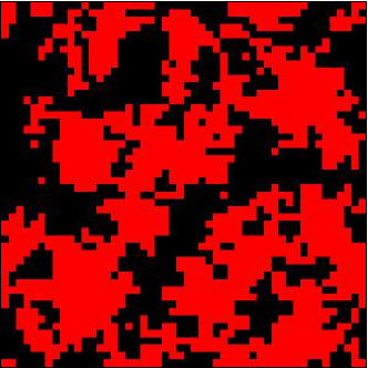
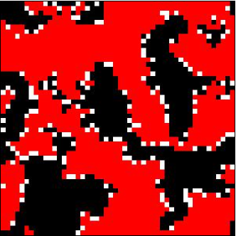
Figure 2: Snapshots of the Voter model (left) and the Bilinguals model (right). Speakers of language A (red), B (black) and bilinguals (white) after 80 time steps starting with a random initial condition.

The second result is related to the role of social networks of increasing complexity. In the first place, small world networks Watts and Strogatz (1998) are considered, which take into account the existence of long range interactions throughout the network. In comparison to the Voter model, where the dynamics reaches a metastable state , bilingual agents restore the processes of domain growth and they speed-up the decay to the absorbing state of language dominance by finite size fluctuations Castelló et al. (2006). The characteristic time, $\tau$ to reach an absorbing state scales with the rewiring parameter  as $\tau\sim p^{-0.76}$.

Secondly, networks with community structure are analyzed, following the algorithm by Toivonen et al. Toivonen et al. (2006). These networks mimic most of the features of real social networks: the presence of hubs, high clustering, assortativity, and mesoscale structure. Communities do not affect substantially the Voter model dynamics, where the system reaches again metastable states. Instead, the presence of communities dramatically affects the AB model Castelló et al. (2007). On the one hand, linguistic domains correlate with the community structure, with bilingual agents connecting agents belonging to different communities, leading to trapped metastable states. The analysis of the lifetime distributions to reach an absorbing state shows that there is no characteristic time for the dynamics (Fig. 3): trapped metastable states are found at arbitrary long times, which lead to scenarios of long time language segregation. Notice that the change in the interface dynamics found in two-dimensional lattices mentioned above when introducing bilingual agents, from interfacial noise to curvature reduction, is at the basis for the change of behavior observed in complex networks .

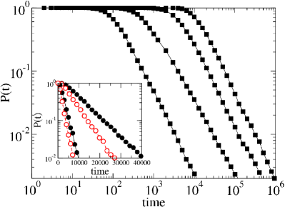
Figure 3: Fraction of alive runs in time for networks with communities (solid symbols) for the AB model (double logarithmic plot). The system sizes are $N=100$, $400$, $2500$, $10000$ from left to right, with averages taken over different realizations of the network ($400$-$5000$ depending on system size), with $10$ runs in each. Inset: same plot for networks with communities (solid symbols) and randomized networks (empty symbols) for the Voter model (semilogarithmic plot). The system sizes are $N=2500$, $10000$. Averages are taken over $100$ different realizations of the networks, with $10$ runs in each. From Ref. Castelló et al. (2007).

The AB model has also been compared to the Naming Game restricted to two conventions (2c-Naming Game) Baronchelli et al. (2007); Castelló et al. (2009). The general Naming Game Steels (1995) describes a population of agents playing pairwise interactions in order to negotiate conventions, i.e., associations between forms and meanings, and elucidates the mechanisms leading to the emergence of a global consensus among them. In the case of two conventions, the Naming Game can be also interpreted as a language competition model with two non-excluding options. The AB model and the 2c-Naming Game are found to be equivalent in the mean field approximation. However, the main result concerns the fact that, when these are extended incorporating a parameter $\beta$ which describes the inertia of the agents to abandon an acquired language, they show an important difference with respect to the existence of an order-disorder transition. While the 2c-Naming Game features an order-disorder transition between consensus and stationary coexistence of the three phases present in the system Baronchelli et al. (2007), in the AB model such a transition does not exist Castelló et al. (2009).

II.2.3 Mira et al. model

The works of Mira et al. Mira and Paredes (2005); Mira et al. (2011) introduce the category of bilinguals, in the particular but relevant case in which two languages are relatively similar to each other and partially mutually intelligible. In such a situation any speaker of e.g. the speaking community B can learn the language of the other speaking community A with a small effort, thus becoming a member of the bilingual community AB. In practice, this is described in the model through a transition probability, to switch from monolingual B to a bilingual community AB, which is relatively large compared to that of the opposite transition, as discussed below. This changes the dynamics in such a way that stable coexistence is possible.

The model may actually be given more general interpretations, since there may be situations in which the transition from a monolingual community B to the bilingual community AB is very probable or easiest to carry out for reasons other than linguistic similarity, e.g. tight economical needs which requires both languages or social policies which favor or push B speakers to learn language A.

The model describes the time evolution of the fractions $x_{A}$ and $x_{B}$ of speakers in the monolingual communities A and B and the analogous fraction $x_{AB}$ for the bilingual community AB. In the approximation of a constant total population, $x_{A}+x_{B}+x_{AB}=1$, one can eliminate the variable $x_{AB}$, obtaining

$$\dot{x}_{A}\! = \!(1-x_{A})(1-k)s_{A}(1-x_{B})^{a}-x_{A}(1-s_{A})(1-x_{A})^{a}\,,$$

$$\dot{x}_{B}\! = \!(1-x_{B})(1-k)(1-s_{A})(1-x_{A})^{a}-x_{A}s_{A}(1-x_{B})^{a}\,,$$ (11)

which reduce to Eqs. (II.1.1) of the AS model for $k=0$. Here the normalization for the language status $s_{A}+s_{B}=1$ has been assumed, so that the actual parameters of the model are $a$, $k$ and $s_{A}$. The closer the parameter $k$ is to one, the more probable is the transition from monolingual B to bilingual AB. Different types of stable equilibrium states have been shown to exist in the phase-plane of the model Mira and Paredes (2005); Mira et al. (2011), including some with non-zero bilingual community size $x_{AB}>0$ even for $s_{A}\neq 1/2$, i.e. when one of the languages is favored by a higher status. In order for this condition to happen a sufficiently large value of $k$ is needed Mira et al. (2011).

II.2.4 Lotka-Volterrra like models

In Ref. Pinasco and Romanelli (2006) a Lotka-Volterra-like dynamical model is introduced, which provides a counter-example to the conclusions of the AS model (which predicts the extinction of one of the two competing languages in a broad range of values of the prestige $s$ and volatility $a$ parameters). A main ingredient of the model is the introduction of population dynamics with different Malthus rates $\alpha_{A}$ and $\alpha_{B}$ for the two populations A and B. The dynamical equations read

$$\dot{x}_{A}\! = \!c\,x_{A}x_{B}+\alpha_{A}x_{A}\left(1-\frac{x_{A}}{K_{A}}\right)\,,$$

$$\dot{x}_{B}\! = \!-c\,x_{A}x_{B}+\alpha_{B}x_{B}\left(1-\frac{x_{B}}{K_{B}}\right)\,,$$ (12)

where $c$ measure the switch rate from language B to language A, while the carrying capacities $K_{A}$ and $K_{B}$ represent the maximum population sizes allowed in case of isolated populations ($c=0$). The language with lower status --- in the present case language B since it is assumed that $c>0$ --- is shown to be able to survive, as long as its corresponding reproduction rate is higher than its language disappearance rate, i.e. if $cK_{B}<\alpha_{B}$. This system presents a stable equilibrium solution in which both communities survive ($x_{A},x_{B}>0$).

As noticed in Ref. Kandler and Steele (2008), the equilibrium value of the population size $x_{A}$ is larger than the maximum allowed value $K_{A}$ for population A. In order to overcome this problem, Kandler et al. Kandler and Steele (2008) have proposed some different models. In particular, they introduced a model with a common carrying capacities $K$ for the two language communities, in the sense that in principle both the communities could reach the same maximum population size $K$. To take into account the fact that in practice the resources actually available to a community are limited by those already used by the other community, their model (in its zero-dimensional version) is defined by the following equations,

$$\dot{x}_{A}\! = \!c\,x_{A}x_{B}+\alpha_{A}x_{A}\left(1-\frac{x_{A}}{K-x_{B}}\right)\,,$$

$$\dot{x}_{B}\! = \!-c\,x_{A}x_{B}+\alpha_{B}x_{B}\left(1-\frac{x_{B}}{K-x_{A}}\right)\,.$$ (13)

Notice that while the transition between A and B communities is regulated by the same Lotka-Volterra-type rate of the model described in Eq. (II.2.4), the Verhulst terms in the population dynamics part of the equations now contain the effective carrying capacities $K_{A}(t)=K-x_{B}(t)$ and the analogous one for population B, which prevent the population sizes from overcoming the carrying capacity $K$. However, with this change the coexistence equilibrium state is lost again and only one community can survive asymptotically. The addition of heterogeneity to the model can change things substantially, as discussed below in Sec. III.

The model was then generalized to include the bilingual community size Kandler (2009); Kandler and Steele (2008). The transition dynamics is similar to that of the Minett and Wang model but effective carrying capacities of the population dynamics part are designed in a way similar to those used above in Eqs. (II.2.4). It was still found that the presence of bilingualism does not allow the coexistence of two languages asymptotically and that bilinguals represent the interface between the two monolingual communities; however, the presence of bilinguals can in some cases prolong significantly the extinction time.

III Models with geography

The importance of physical geography, e.g. the presence of water boundaries and mountains, for the evolution and dispersal of biological species is well known Lomolino et al. (2006). In cultural diffusion, both physical and political boundaries have to be taken into account. Furthermore, other factors of dynamical or economical nature, related to e.g. to the features of the landscape, can modify the otherwise homogeneous cultural spreading process.

The geographical models considered below Kandler and Steele (2008); Patriarca and Heinsalu (2009); Patriarca and Leppänen (2004) are extensions of the 0-dimensional AS model to spatial domains. In all cases some geographical inhomogeneities are taken into account, related to the underlying political, economical, or physical geography.

III.1 Inhomogeneous cultural diffusion

Inhomogeneous cultural diffusion can be modeled by adopting space (and time) dependent transition rates for the switching between different languages.

In the model introduced in Ref. Patriarca and Leppänen (2004) the speakers of two communities with different languages A and B can diffuse freely across a two-dimensional domain $Z$, divided symmetrically into two regions $\alpha$ and $\beta$. The border between the regions, which could represent e.g. political or geographical factors, is assumed to influence the communication between speakers in such a way that language A is more influential in zone $\alpha$ and language B in zone $\beta$. The reaction dynamics is similar to that of the AS model, with the crucial difference that (1) there is free homogeneous diffusion through the domain $Z=\alpha+\beta$ and (2) each speaker is only affected by the other speakers who are in the same region where the speaker is. The AS dynamics is modified as follows,

$$\frac{\partial f_{A}({\bf r},t)}{\partial t} = \Delta f_{A}({\bf r},t)+R({\bf r},t)\ ,$$

$$\frac{\partial f_{B}({\bf r},t)}{\partial t} = D\Delta f_{B}({\bf r},t)-R({\bf r},t)\ ,$$

$$R({\bf r},t) = \left[s_{A}\,\xi_{A}^{\,a}({\bf r},t)f_{B}({\bf r},t)-s_{B}\,\xi_{B}^{\,a}({\bf r},t)f_{A}({\bf r},t)\right]\ ,$$ (14)

where $\mathbf{r}=(x,y)$, $\Delta$ is the Laplacian in two dimensions, $D$ the diffusion coefficient, $f_{A}$ and $f_{B}$ the population density of the speaking community A and B, respectively, and $s_{i}$ ($i={A},{B};s_{A}+s_{B}=1$) maintain the same meaning of the language status. The terms $\xi_{i}({\bf r},t)$ in the reaction rate $R({\bf r},t)$ are the fractions of speakers of language $i$ at time $t$ in the same region ($\alpha$ or $\beta$) where a speaker with position ${\bf r}$ is,

$$\xi_{i}({\bf r},t) = {N_{i}^{(\alpha)}({\bf r},t)}/[N_{A}^{(\alpha)}({\bf r},t)+N_{B}^{(\alpha)}({\bf r},t)]~{}~{}~{}~{}\mathrm{if}~{}\mathbf{r}\in\alpha\,,$$ (15)

$$= {N_{i}^{(\beta)}({\bf r},t)}/[N_{A}^{(\beta)}({\bf r},t)+N_{B}^{(\beta)}({\bf r},t)]~{}~{}~{}~{}\mathrm{if}~{}\mathbf{r}\in\beta\,,$$ (16)

$$N_{i}^{(\alpha)}({\bf r},t) = \int_{\alpha}dx^{\prime}dy^{\prime}f_{i}({\bf r}^{\prime},t)\,,~{}~{}N_{i}^{(\beta)}({\bf r},t)=\int_{\beta}dx^{\prime}dy^{\prime}f_{i}({\bf r}^{\prime},t)\,,~{}~{}i={A},{B}\,.$$ (17)

The model exhibits stable equilibrium with both languages surviving in the two different regions $\alpha$ and $\beta$, also for very different language status, if the two populations are initially separated on the opposite sides of the boundary.

Another example of inhomogeneous language spreading modeling is provided by the model introduced in Ref. Kandler and Steele (2008), where the transition rate $c$ in Eqs. (II.2.4) is allowed to vary in space, i.e. $c\to c({\bf r})$, and diffusion is taken into account. This analogously models a situation in which the two languages have a higher status in different spatial domains. The equations read

$$\frac{\partial f_{A}({\bf r},t)}{\partial t} = D_{A}\Delta f_{A}({\bf r},t)+c({\bf r})f_{A}({\bf r},t)f_{B}({\bf r},t)+\alpha_{A}f_{A}({\bf r},t)\!\!\left[1-\frac{f_{A}({\bf r},t)}{K\!-\!f_{B}({\bf r},t)}\right]\!,~{}~{}~{}~{}$$

$$\frac{\partial f_{B}({\bf r},t)}{\partial t} = D_{B}\Delta f_{B}({\bf r},t)-c({\bf r})f_{A}({\bf r},t)f_{B}({\bf r},t)+\alpha_{B}f_{B}({\bf r},t)\!\!\left[1-\frac{f_{B}({\bf r},t)}{K\!-\!f_{A}({\bf r},t)}\right]\!\!.~{}~{}~{}~{}$$ (18)

The model predicts survival of both languages in the two different regions for suitable forms of the function $c({\bf r})$.

It is noteworthy that Kandler et al. applied their geographical models in real situations, to test different social strategies planned for defending the survival of Britain’s Celtic languages Kandler (2009); Kandler and Steele (2008); Kandler et al. (2010). For further details and data source references see Ref. Kandler et al. (2010). It is also worth pointing out that the geographical character of these models may be given a wider interpretation in terms of social space. For instance, the $x$ coordinate may represent age, different income classes, or different social environments (e.g. workplace versus administration, workplace versus home, etc.). Thus, while in all these cases there is actual competition between languages everywhere, in practice each language eventually may turn up to be successful in and therefore characterize a different specific social domain. The diversity of different languages or language features or their ability to find a suitable niche where to be successful is crucial to the survival of any minority language.

III.2 Inhomogeneous human dispersal

The model introduced in Ref. Patriarca and Heinsalu (2009) can be considered to be complementary to those discussed in the previous section, in the sense that it assumes a homogeneous switching rate in parallel with an inhomogeneous diffusion. It can be noticed that while inhomogeneous diffusion is typically caused by factors related to the physical geographic features of the underlying landscape, it can also be due e.g. to political boundaries or natural borders between regions with very different economical features. It turns out that even such non-cultural features can strongly influence the evolution and final distribution of cultural traits.

In the continuous limit the model assumes a dynamics of a reaction-diffusion type, described by

$$\frac{\partial f_{1}}{\partial t} = R(f_{1},f_{2})-\nabla\cdot\left(\,\mathbf{F}f_{1}\right)+\nabla\cdot(D\nabla f_{1})+\alpha f_{1}\left(1-\frac{f_{1}+f_{2}}{K}\right)\ ,$$ (19)

$$\frac{\partial f_{2}}{\partial t} = -R(f_{1},f_{2})-\nabla\cdot\left(\,\mathbf{F}f_{2}\right)+\nabla\cdot(D\nabla f_{2})+\alpha f_{2}\left(1-\frac{f_{1}+f_{2}}{K}\right)\ ,$$ (20)

$$R(f_{1},f_{2}) = k\left(s_{1}f_{1}^{\,a}f_{2}-s_{2}f_{2}^{\,a}f_{1}\right)\,.$$ (21)

Here the first term on the right hand side of Eqs. (19) and (20) is the reaction term $R$, which can be recognized from Eq. (21) to be formally identical to that of the AS model, if the population fractions are replaced by the population densities. Inhomogeneous diffusion can be due to the advection term containing the external ‘‘force field’’ $\mathbf{F}(x,y)=(F_{x}(x,y),F_{y}(x,y))$ as well as to an inhomogeneous diffusion coefficient $D=D(x,y)$. The model also contains logistic terms with Malthus rate $\alpha$ and carrying capacity $K$, which introduces a negative competitive coupling $\propto-f_{1}f_{2}$. Notice that for equal dispersal and growth properties, the total population density $f=f_{1}+f_{2}$ follows a standard diffusion-advection-growth process,

$$\frac{\partial f}{\partial t}=-\nabla\cdot[\,\mathbf{F}f]+\nabla\cdot(D\nabla f)+\alpha f\left(1-\frac{f}{K}\right)\,.$$ (22)

The results of Ref. Patriarca and Heinsalu (2009) can be summarized as follows. First, inhomogeneities in the initial distributions are crucial for the final state, e.g. broader initial distributions represent a disadvantage for small population growths ($\alpha\to 0$) while they can become an advantage for large enough values of $\alpha$. Secondly, also boundary conditions are relevant in the competition process, e.g. the vicinity of reflecting boundaries definitely favors the survival of a language for low growth rates. Finally, geographical barriers such as mountains or rivers can create a refugium where a linguistic population with lower status can survive with a stable finite density, even in the presence of an in-flux of speakers of a higher-status language.

As in the previous section, similar considerations apply also to these specific models describing human dispersal about possible more general interpretations as models of dispersal in social space, e.g., through different social classes.

IV A Game-Theoretical Model: Bilinguals as a Minority Population

IV.1 Introductory remarks

The AS model Abrams and Strogatz (2003), where the languages $A$ and $B$ compete for speakers, is not a good analytical tool to study most of the multilingual societies, as we know them today. The AS model seems to be more appropriate to describe the language competition that took place during the historical period of emergence of nation-states, typically during the 18th and 19th century in Europe. This is the period in which the nationalist program is about to be accomplished: the consolidation of a national market, with precise borders, free of internal restrictions to economic activities, and an increasing demand for a unique national language that would facilitate those activities and help develop a national culture and identity Hobsbawm (1992). Some societies, nevertheless, in Europe and elsewhere, resisted that shift to language uniqueness. Extensions of the AS model have been developed to understand the existence of those multilingual societies (see sections III.1 and III.2, and Refs. Minett and Wang (2008); Mira and Paredes (2005); Patriarca and Leppänen (2004); Pinasco and Romanelli (2006)). The Lotka-Volterra type of models of language shift Kandler and Steele (2008); Kandler et al. (2010) describe fairly well the historical shift to English of Scottish Gaelic and Welsh, that converted these two vernacular languages into two minority languages.

Here, we shall consider a society with two languages, $A$ spoken by all its members, and $B$ spoken by a small proportion $\alpha$. Thus, $\alpha$ denotes the proportion of bilingual speakers and $(1\!-\!\alpha)$ that of the monolingual ones. As examples of this situation, we can consider: in Wales, Welsh and English; in Scotland, Scottish Gaelic and English; in the Basque Country, Basque and French in the French part and Basque and Spanish in the Spanish part; in Brittany, Breton and French; Sami and Swedish, Norwegian and Russian in the Sami society; Frisian, spoken in the province of Friesland in The Netherlands, competing with Dutch; Maori and English in New Zealand and Australia; Native American languages (Quechua, Aymará, Guarani, among others) and English, Spanish, French, Portuguese and Dutch in America; languages from the Russian Federation competing with Russian. See Ref. Fishman (2001) for more examples.

We could either assume a population of constant size or allow for changes in the size. In the latter case, any new individual added to the society (say an immigrant) would, most likely, learn at least $A$. But in both cases the proportion of individuals who would speak $A$, in the type of society we are dealing with, would always be almost, or just, 100%. Hence, in those societies, there is no dynamics for language $A$ of any relevance. Only the dynamics of language B matters; and, therefore, to keep diversity, only the use of B matters.

We will investigate the language conventions of bilingual speakers by means of game-theoretic tools. As a methodological procedure, we might think that our analysis will deal with the stable equilibria obtained by some of the models used in Refs. Patriarca and Leppänen (2004); Mira and Paredes (2005); Pinasco and Romanelli (2006); Minett and Wang (2008), where it is formally shown that A and B may coexist. We want to study the language used in the interactions between bilingual speakers that occur outside the traditional geographical areas of B studied in section III.1 Patriarca and Leppänen (2004), and ask: will the language conventions developed by the bilingual speakers use the minority language B and therefore keep up the language diversity?

IV.2 The Language Conversation Game (LCG): Iriberri-Uriarte Model

The model proposed by Iriberri and Uriarte [13] consists of a game played by two individuals (at least one should be bilingual) to decide the language that will be used in the conversation that takes place during an interaction. The model satisfies the following set of assumptions.

IV.2.1 Assumptions

Assumption 1 (A.1).

Imperfect information: Nature or Chance chooses first the actual realization of the random variable that determines the type of each speaker (i.e. bilingual or monolingual). But each speaker knows only his own type. That is, a bilingual speaker does not know, ex-ante, the bilingual or monolingual type of the agent she will interact with. We assume, on the other hand, that the probability distribution, $\alpha$ and $(1-\alpha)$, is common knowledge among all the agents in the society

Assumption 2 (A.2)

Linguistic Distance: A and B are linguistically very distant, so that successful communication is only possible when the interaction takes place in one language.

Assumption 3 (A.3)

Language loyalty: Bilingual speakers prefer to use B.

Assumption 4 (A.4)

Payoffs: For a given proportion $\alpha<1-\alpha$, we assume the following payoff ordering: $m>n>c>0$. The maximum payoff $m$ is obtained when bilingual speakers coordinate in their preferred language B. Bilingual or monolingual players might coordinate on the majority language $A$; in that case, we will assume both players get payoffs equal to $n$, because this was a voluntary coordination or choice. Then $(n-c)$ is the payoff to a bilingual player who, having chosen $B$, is matched to someone monolingual (or bilingual) who uses language $A$ and is therefore forced to speak $A$; $c$ denotes the frustration cost felt by this bilingual speaker.

Assumption 5 (A.5)

Frustration Cost: $c<(m-n)\alpha/(1-\alpha)$. The bilingual’s frustration cost is smaller than the weighted benefit.

IV.2.2 Discussion of the assumptions

Notice that A.1 does not allow the existence of a geographical linguistic partition, as it is assumed in Ref. Patriarca and Leppänen (2004), since inside the historical areas where B is widely used, there will exist almost perfect information about the bilingual or monolingual nature of their inhabitants. A.1 tries to capture the use of $B$ outside the strongholds of $B$, in, so to say, the urban domains. We should take into account that, often, one of the consequences of a language contact situation is that even the accents, as signals that would reveal who speaks $B$ and who does not, are erased. If we eliminate A.1 and assume perfect information and the rest of assumptions, it is easy to see that bilingual speakers would coordinate in $B$. Assumption A.2 avoids the linguistic similarities between A and B assumed in Ref. Mira and Paredes (2005). If we assume language similarity, then conversations could take place using both $A$ and $B$, bilingual speakers would not be forced to change necessarily from $B$ to $A$, and there would not be any frustration cost. If, instead of A.5, we assume $c\geq(m-n)\alpha/(1-\alpha)$ while keeping the other assumptions, then it can be shown that the language used in equilibrium would be $A$. See also Ref. Iriberri and Uriarte (2012).

IV.2.3 Pure Strategies

Let us consider a bilingual speaker who must decide, under imperfect information, which language is going to use in an interaction which is about to occur. Simplifying things, we could say that the bilingual speaker expects to be involved in two exclusive events: a matching with another bilingual speaker (which will occur with probability $\alpha$) and a matching with a monolingual speaker (which will occur with probability $1-\alpha$). We could also simplify the set of strategies that any bilingual speaker may play to the following two:

$\mathbf{s}_{\mathbf{1}}$:

Use always B, whether you know for certain you are speaking to a bilingual individual or not.

$\mathbf{s}_{\mathbf{2}}$:

Use B only when you know for certain that you are speaking to a bilingual individual; use A, otherwise.

Note that strategy $\mathbf{s}_{\mathbf{1}}$ reveals the bilingual nature of the speaker. Strategy $\mathbf{s}_{2}$, on the other hand, hides the bilingual nature of the speaker. Its purpose is to avoid the frustration cost $c$ of assumption A.4.

In the present paper, we study the normal form of the LCG. A complete description of the LCG is given by the extensive form presented in Ref. Iriberri and Uriarte (2012).

The language associated to each pure strategy profile is given by the following matrix:

$$\mathbf{s}_{1}$$

Note that since players have no perfect information about the type of the opponent, they might use either B or A in the interaction. That is, if both bilingual speakers hide their type by choosing $\mathbf{s}_{\mathbf{2}}$, then they will use in the interaction their less preferred language A. In the other three cases they will use B, because at least one speaker is revealing the bilingual identity.

IV.2.4 Expected Payoffs

The (mythical) player called Nature or Chance chooses, with probability $\alpha$, that the bilingual speaker interacts with another bilingual speaker, to play the game described in Fig. 4, in which, by assumption A.4, strategy $\mathbf{s}_{\mathbf{1}}$ is weakly dominant.

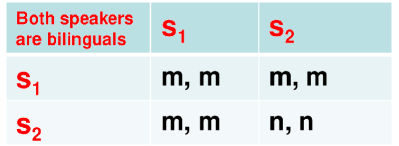
Figure 4: The game to be played in the event in which two bilingual speakers are matched. Notice that $s_{1}$ is weakly dominant.

Nature chooses, with probability $1-\alpha$, that the bilingual speaker interacts with a monolingual speaker, to play the game described in Fig. 5, in which, by assumption A.4, $\mathbf{s}_{\mathbf{2}}$ is strictly dominant. The monolingual agent does not make choices and gets $n$.

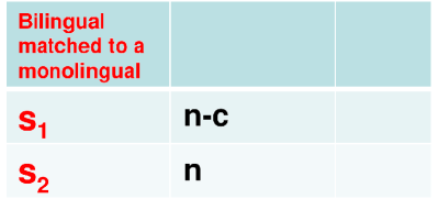
Figure 5: The game to be played in the event in which a bilingual speaker is matched to a monolingual. Notice that $s_{2}$ is strictly dominant.

If a bilingual speaker chooses strategy $\mathbf{s}_{\mathbf{1}}$, then, no matter the choices of the other bilingual player, the expected payoff is $\alpha m+(1-\alpha)(n-c)$; if the choice is $\mathbf{s}_{\mathbf{2}}$, then, against $\mathbf{s}_{\mathbf{1}}$, the expected payoff will be $\alpha m+(1-\alpha)n$ and, against $\mathbf{s}_{\mathbf{2}}$, $n$. The resulting matrix of expected payoffs of the LCG played by two bilingual speakers will, therefore, be symmetric:

$$\mathbf{s}_{\mathbf{1}}$$

, ,

, ,

Matrix of Expected Payoffs

IV.3 Evolutionary Setting

The LCG will now be viewed as a population game. To this end, let us assume that the bilingual population consists of a large, but finite number of individuals, who play a certain pure strategy $s_{\mathbf{i}}$, ($i=1,2$), in a two-player game. The members of the bilingual population play the LCG having $S=\{s_{1},s_{2}\}$ as their common strategy set. The interactions are modelled as pairwise random matching between agents of the bilingual population; that is, no more than two (randomly chosen) individuals interact at a time. The interactions take place continuously over time. Let $N$ be the total population of bilingual speakers in the society, and $x=\frac{\mathbf{N}_{1}}{\mathbf{N}}$ the proportion of bilingual agents playing the pure strategy $s_{\mathbf{1}}$ at any point t in time (time dependence is suppressed in the notation). In this setting, a mixed strategy is interpreted as a population state that indicates the bilingual population share of agents playing each pure strategy. On the other hand, the payoffs of the game should not be interpreted as biological fitness, but as utility. Under assumptions A.1-A.5, we get the following result.

Proposition. There exists a mixed strategy Nash equilibrium in which the bilingual population plays $s_{\mathbf{1}}$ with probability $x^{\ast}=1-\frac{c(1-\alpha)}{\alpha(m-n)}$. This equilibrium is evolutionary stable — that is $x^{\ast}$ is a language convention built by the bilingual population — and asymptotically stable in the associated one-population Replicator Dynamics.

Proof: Note that the LCG has the strategic structure of a Hawk-Dove Game (with $\mathbf{s}_{\mathbf{1}}$ as Dove and $\mathbf{s}_{\mathbf{2}}$ as Hawk). Thus, it has three Bayesian Nash equilibria: the asymmetric (and unstable) equilibria $(\mathbf{s}_{\mathbf{2}},\mathbf{s}_{\mathbf{1}})$ and $(\mathbf{s}_{\mathbf{1}},\mathbf{s}_{\mathbf{2}})$, and the symmetric mixed strategy equilibrium $(x^{\ast},1-x^{\ast})=$ $(1-\frac{c(1-\alpha)}{\alpha(m-n)},\frac{c(1-\alpha)}{\alpha(m-n)})$, with $x^{\ast}\in(0,1)$. To see that the latter equilibrium is evolutionary stable, see Ref. Weibull (1995). The single population Replicator Dynamics is as follows:

$$\overset{\cdot}{x}\text{ }=[\alpha(m-n)(1-x)-c(1-\alpha)]x(1-x)\,.$$

Notice that in $x^{\ast}$, $\alpha(m-n)(1-x)-c(1-\alpha)=0$ and so $\overset{\cdot}{x}=0$. We can see that for any $0<x<1-\frac{c(1-\alpha)}{\alpha(m-n)}$, $\overset{\cdot}{x}$ increases toward $x^{\ast}$, and for any $1>x>1-\frac{c(1-\alpha)}{\alpha(m-n)}$, $\overset{\cdot}{x}$ decreases toward $x^{\ast}\blacksquare$.

IV.3.1 Interpretation

Language $B$ is spoken in the asymmetric equilibria $(\mathbf{s}_{\mathbf{2}},\mathbf{s}_{\mathbf{1}})$ and $(\mathbf{s}_{\mathbf{1}},\mathbf{s}_{\mathbf{2}})$, but these equilibria are unstable and, hence, we must rule them out. Thus, we are left with the evolutionary and asymptotically stable equilibrium $x^{\ast}$. Since $x^{\ast}\in(0,1)$, $\mathbf{s}_{\mathbf{1}}$ and $\mathbf{s}_{\mathbf{2}}$ are played by non-zero proportions of bilingual speakers. That is, the bilingual population is optimally partitioned in two subpopulations: $N_{1}^{\ast}=N[1-\frac{c(1-\alpha)}{\alpha(m-n)}]$ and $N_{2}^{\ast}=N\frac{c(1-\alpha)}{\alpha(m-n)}$. The former group is composed of agents who play strategy $s_{\mathbf{1}}$ and the latter of those who play $s_{\mathbf{2}}$. Hence, the bilingual agents in $N_{2}^{\ast}$ do not use $B$ in the interactions among themselves. Only when they interact with agents of $N_{1}^{\ast}$ will they use $B$.

Thus, in equilibrium, the population of bilingual speakers will speak both $A$ and $B$ in the interactions between themselves; the level of use of $B$ depends on the relative size of $N_{1}^{\ast}$.

IV.4 Concluding remarks

The mixed equilibrium $x^{\ast}$ is compatible with almost all the possible levels of use of $B$: from the lowest, when $x^{\ast}$ is almost $0$ and therefore $N_{2}^{\ast}$ approaches $N$, so that bilingual speakers will mostly speak $\mathit{A}$ between them; to the highest, when $x^{\ast}$ is almost $1$ and so bilingual speakers will be almost all speaking their preferred language $B$. Hence we cannot give a sharp answer to the question posed in the introductory remarks in Sec. IV.1. We can only say that language diversity is not safe in this equilibrium.

Our prediction is that there is a tendency towards a situation in which $N_{2}^{\ast}>N_{1}^{\ast}$, and that the use of B will always face the danger of being reduced to marginal levels outside the traditional areas. Many factors will intervene, some of them from outside the model. Among others, imperfect information, the dominance of A in formal and informal usages of the language, and the politeness norms that would advice the use of (the Hawk strategy) $\mathbf{s}_{\mathbf{2}}$. Bilingual speakers playing $\mathbf{s}_{\mathbf{2}}$ will hurt each other because they end up speaking the less preferred language (see the language matrix above). This might explain the difficulties observed by Fishman (2001) Fishman (2001). The actual lower bound to the use of B will be near to that set by the communities living in the geographical areas where $\mathit{B}$ is strong and where interactions occur with almost perfect information Patriarca and Leppänen (2004). See Ref. Iriberri and Uriarte (2012) for a more complete analysis.

V Conclusions

We have revisited several approaches used to study the dynamics of two competing languages. The main question addressed is whether the competition leads to the coexistence or on the contrary to the prevalence of a majority language. The seminal work of the AS model considers speakers of two languages without the possibility of bilinguals. In this case, the stationary configurations depend on the volatility, that is, how easy is to change language use depending on the local density of speakers. When the volatility is high ($a<1$), i.e., the probability is larger than the linear case, coexistence is the stationary solution where the percentage of speakers of each language depends on the prestige. When the volatility is low ($a>1$), the systems converges to the dominance of one of the languages and the extinction of the other. The presence of bilinguals and network of interactions (Bilinguals model) change the boundaries separating the different regimes, but the overall picture remains similar. Physical and/or political boundaries have been shown to allow for coexistence as long as the two communities are separated. There have been also attempts to show the coexistence of monolingual speakers in population dynamic models and the stability of bilingual communities. Finally, by means of a game theoretical approach, we have analyzed the case of language competition when one of languages is known by all the agents while the other is only spoken by a minority.

Despite the efforts to understand the different mechanisms of language competition, an overall clear picture on the question of coexistence (or not) or multilingual communities is still missing. In this respect empirical works should provide evidence and guidance to improve current models. The original data in Ref. Abrams and Strogatz (2003) on the evolution of the total number of speakers has triggered the research line so far. Recent research Kandler et al. (2010) using empirical data on Britain’s Celtic languages with good spatial and temporal resolution should be taken as a motivation for further studies. We anticipate that future research will address how spatio-temporal patterns emerge from the competition of local interaction with global signals (e.g., prestige, language policies).