Quantitative analysis of pedestrian counterflow in a cellular automaton model

Abstract

Pedestrian dynamics exhibits various collective phenomena. Here we study bidirectional pedestrian flow in a floor field cellular automaton model. Under certain conditions, lane formation is observed. Although it has often been studied qualitatively, e.g. as a test for the realism of a model, there are almost no quantitative results, neither empirically nor theoretically. As basis for a quantitative analysis we introduce an order parameter which is adopted from the analysis of colloidal suspensions. This allows to determine a phase diagram for the system where four different states (free flow, disorder, lanes, gridlock) can be distinguished. Although the number of lanes formed is fluctuating, lanes are characterized by a typical density. It is found that the basic floor field model overestimates the tendency towards a gridlock compared to experimental bounds. Therefore an anticipation mechanism is introduced which reduces the jamming probability.

I Introduction

From a physical point of view, human crowds are many-body systems which show many interesting collective effects. Examples are jamming at bottlenecks, density waves, flow oscillations, pattern- and lane formation Schadschneider01 . The latter terms the effect that pedestrians in a crowd segregate spontaneously according to their desired walking direction. Related phenomena can not only be observed in pedestrian dynamics but also in other physical systems. For instance in granular media, the components assort according to their size when vibrations are applied to the system granular1 . The effect occurs particularly in driven systems Schmittmann199845 , e.g., in complex plasmas PhysRevLett.102.085003 , molecular ions 0295-5075-63-4-616 and colloidal suspensions PhysRevE.65.021402 ; nature_colloidal ; rex07 . For the latter also an order parameter for the detection of lanes was introduced which we are going to adopt for pedestrian crowds (cf. Section II.2). More on the phase diagram and the lane transition of colloids can be found in Ref. lane_colloidol_hyd ; lane_colloidol_cont .

Nevertheless, the phenomenon is best known in pedestrian counterflow from everyday experience although experimental or empirical studies are quite rare NavinW ; empir1 ; empir3 ; Suma2012248 ; empir2 . The effect can be understood as a self-organization process, where pedestrians try to minimize the contact with other pedestrians, especially if they have a different desired walking direction. The mechanism which leads to segregation into distinct lanes is not fully understood. A possible explanation could be a fundamental left-right asymmetry, i.e., people prefer to walk either on the right or on the left. But note that this is not necessary for the effect. The symmetry can also break spontaneously if certain assumptions are made, for instance that people tend to follow each other.

Computer simulations of bidirectional pedestrian movement (counterflow) are made frequently cam10 ; cam5 ; cam6 ; cam8 ; burstedde01 ; jam_trans_1 ; jam_trans_3 ; jam_trans_2 ; jam_trans_4 ; jam_trans_5 ; springerlink:10.1007/978-3-540-79992-4_75 ; Weng2007668 ; empir2 ; socfor1 ; helbing01 ; Jiang09 ; makro_lanes . Lane formation can be reproduced qualitatively schadschneider_collective ; helbing01 and is often used as a validation of a model, but there are no quantitative descriptions of the formation process or the properties of lanes. Even a description which goes beyond the statement that lanes are present in the system or even comparisons with empirical data are extremely rare empir2 ; crawling . Another focus related to bidirectional flow is on the jamming transition jam_trans_1 ; jam_trans_3 ; jam_trans_2 ; jam_trans_4 ; jam_trans_5 , i.e. the transition to a state where no movement is possible anymore (gridlock). However, there is no empirical evidence for such a transition and recent experiments showed that the lower density limit for the transition is larger than 3.5 Persons/m² zhang02 .

II Definitions

II.1 Floor Field Cellular Automaton Model

The Floor Field Cellular Automaton (FFCA) model burstedde01 ; kirchner02 ; KirchnerNS03 is defined on a two-dimensional square lattice where each cell can be occupied by at most one particle (pedestrian). In every timestep, each particle is allowed to stay at its current position or to move to one of the neighboring cells given that the destination cell is not occupied by another particle. This is done synchronously for all particles (parallel update). The number of nearest neighbors on the lattice can either be four (von Neumann neighborhood, cf. Fig. 1) or eight (Moore neighborhood). One can estimate the area assigned to each cell by taking the reciprocal of the maximal possible density $\rho_{\text{max}}$ in a pedestrian crowd. Although the empirical value of $\rho_{\text{max}}$ is not known very well Schadschneider01 , a common value often used in cellular automata is $\rho_{\text{max}}=6.25~{}\text{Persons}/\text{m}^{2}$ which leads to a size of $0.4\times 0.4~{}\text{m}^{2}$ per cell kirik07 ; hua10 ; dijkstra02 . The length of one timestep can be estimated by comparing it with the typical reaction time of a pedestrian. This leads to a value of roughly 0.3 seconds for one timestep.

Figure 1: Illustration of the transition probabilities in the von Neumann neighborhood for a particle located at $(i,j)$. In the Moore neighborhood the four corner cells would have a transition probability different from zero.

The movement of particles is defined by transition probabilities $p_{ij}$ which (for the model variant Suma2012248 studied here) are given by

$$p_{ij}= \frac{q_{ij}}{\sum_{i,j}q_{ij}}$$ (1)

$$q_{ij}= \exp\left(k_{\mathrm{S}}S_{ij}+k_{\mathrm{D}}D_{ij}-k_{\mathrm{A}}A_{ij}\right)\xi_{ij}$$ (2)

where $k_{\text{S}}$ and $k_{\text{D}}$ are coupling constants. The factor $\xi_{ij}\in\{0,1\}$ ensures that movement only takes place at allowed sites, i.e., $\xi_{ij}=0$ if the cell $(i,j)$ is not accessible and $\xi_{ij}=1$ otherwise. Inaccessible cells are wall-cells, cells which are occupied by other pedestrians and cells which are not in the geometry or the corresponding neighborhood of the origin-cell. The matrices $S$ and $D$ represent the so-called “floor fields”, where $S$ is the static floor field (SFF), $D$ is the dynamic floor field (DFF) and $A$ is the anticipation floor field (AFF). The latter is the main difference to the standard FFCA burstedde01 ; kirchner02 which corresponds to the choice $k_{A}=0$. The expression

$$V_{ij}=-\left(k_{\mathrm{S}}S_{ij}+k_{\mathrm{D}}D_{ij}-k_{\mathrm{A}}A_{ij}\right)$$ (3)

in the exponential function of eqn. (2) can be interpreted as a time-dependent potential, i.e., movement is prefered into the direction of larger $V_{ij}$.

Bidirectional flow is modelled by two different species of particles which have opposite preferred walking directions. One type of particle, which is called “type A”, is directed towards the right while “type B” particles are directed to the left. In a colloidal suspension these types would correspond to oppositely charged particles.

The underlying geometry is a rectangle of $W\times L$ cells where $W$ and $L$ correspond to the width and the length of the system. A subset of $L$ neighboring cells along the walking direction is called a row and $W$ neighboring cells perpendicular to the walking direction are called a column. The particle positions can be described by a $L\times W$-matrix $\tau_{ij}$ which can be defined as

$$\tau_{ij}(t)=\begin{cases}+1&\text{if~{}there~{}is~{}a~{}particle~{}of~{}type~{}}A\\ -1&\text{if~{}there~{}is~{}a~{}particle~{}of~{}type~{}}B\\ 0&\text{if~{}there~{}is~{}no~{}particle}\end{cases}$$ (4)

on the cell $(i,j)$. The absolute value $|\tau_{ij}|$ corresponds to the usual binary occupation number.

II.1.1 Static Floor Field

The Static Floor Field (SFF) does not change in time and is not influenced by the presence of particles. It contains the information about the preferred direction of motion. Typically it describes the shortest distance to a destination using some metric. In a counterflow situation one can give a very simple expression for the SFF in equation (2) which is

$$S^{A}_{ij}=\begin{cases}+1&\text{if the cell }(i,j)\text{ is to the {right}}\\ -1&\text{if the cell }(i,j)\text{ is to the {left}}\\ 0&\text{otherwise}\end{cases}$$ (5)

for particles of type $A$ and $S^{B}_{ij}=-S^{A}_{ij}$ for particles of type $B$. This means that different types of particles are affected by different SFFs.

II.1.2 Dynamic Floor Field

The Dynamic Floor Field (DFF) was inspired by the motion of ants, who leave a pheromone trace schad_ants . Other ants are able to smell this trail and follow it. This concept is adopted in this model: Each particle which moves from one cell to another leaves a virtual trace, i.e., the DFF value $D_{ij}$ of the origin cell $(i,j)$ increases by 1. This trace acts attracting on other particles due to larger transition probabilities according to equation (2). The effect is that particles have a tendency to follow each other. An important detail is to avoid particles being attracted by their own virtual trace. Therefore, in the calculation of the transition probability in equation (2) the DFF is temporarily reduced by 1 on the last visited cell. In the same manner as the SFF one should use two different DFFs $D_{ij}^{A}$ and $D_{ij}^{B}$ which interact only with particles of type $A$ and $B$, respectively.

The DFF has its own dynamics, namely diffusion and decay. After each timestep, it is updated according to

$$D_{ij}(t+1)=(1-\delta)\Big{[}D_{ij}(t)+\frac{\alpha}{4}\Delta D_{ij}(t)\Big{]}$$ (6)

where

$$\Delta D_{ij}(t) =D_{i,j+1}(t)+D_{i,j-1}(t)$$

$$+D_{i+1,j}(t)+D_{i-1,j}(t)-4D_{i,j}(t)$$ (7)

is a discretization of the Laplace operator. Equation (6) can also be obtained by discretizing

$$\frac{\partial}{\partial t}D_{xy}(t)=\beta\nabla^{2}D_{xy}(t)-\delta D_{xy}(t)$$ (8)

which is the diffusion equation with diffusion constant $\beta=\alpha(1-\delta)/4$ and an extra term for the decay. Here $\nabla^{2}=\partial^{2}/\partial x^{2}+\partial^{2}/\partial y^{2}$ is the usual Laplace operator in two dimensions.

II.1.3 Anticipation Floor Field

When pedestrians are in a counterflow they usually try to avoid collisions by estimating the prospective route of pedestrians with opposite walking direction. This behavior can be imitated by introducing the anticipation floor field Suma2012248 . For particles of type $A$ it is defined as

$$A_{ij}^{A}=\sum_{j^{\prime}}\delta_{1,\tau_{ij^{\prime}}}\lambda^{d_{A}(j,j^{\prime})}$$ (9)

where $\delta_{ij}$ is the Kronecker delta and $\lambda\in(0,1)$ a parameter which controls the range of anticipation. $d_{A}(j,j^{\prime})$ is the minimal number of cells which have to be passed if a particle of type $A$ goes from a cell $(i,j^{\prime})$ to the cell $(i,j)$, only taking steps towards its desired walking direction. The field $A_{ij}^{B}$ for particles of type $B$ is defined analogously. This definition of $A_{ij}$ causes a large value of $A_{ij}^{X}$ ($X\in\{A,B\}$) if there are many particles of type $X$ which are going to tread the cell $(i,j)$ in the nearby future. Particles of the other type $Y$ should avoid this cell, i.e., the AFF acts repulsive (hence the minus sign in eqn. (2)). Note also that only type-$A$ particles are affected by the AFF generated by type-$B$ particles and vice versa.

II.1.4 Update Rules

The update rules which describe the transfer from one timestep to the next are given as follows:

1. Computing the AFF

The AFF is computed in the beginning of every timestep according to eqn. (9) for both types of particles.

2. Choosing destination cells

Each particle chooses a destination cell according to the transition probabilities given in eqn. (1) and (2).

3. Solving conflicts

Conflicts are situations, where $n\geq 2$ particles have chosen the same destination cell. In this case one of the particles is chosen at random to move. For simplicity it is assumed that each particle is chosen with equal probability $1/n$.

4. Movement

Each particle moves to its destination cell. If the destination cell is different from the origin cell, the DFF value of the latter is increased by 1.

5. Diffusion and decay

The values of the DFF are updated according to eqn. (6). If the boundary conditions are not periodic, it is assumed that the DFF is zero beyond the boundary, i.e., $D_{ij}=0$ if $i\notin\{1,\cdots,W\}$ or $j\notin\{1,\cdots,L\}$.

Note that rule 3 for dealing with conflicts can be generalized by introducing a friction parameter burstedde01 ; kirchner02 ; KirchnerNS03 or by coupling with evolutionary games evolutionary_game_friction ; evolutionary_game_friction2 ; evolutionary_game_friction3 . However, here we will only study the simplest version as described above since no indication was found that the way of dealing with conflicts has a qualitative effect on lane formation nowak_lanes .

II.2 Order Parameter for Lane Formation

An order parameter which indicates the presence and absence of lanes has to detect inhomogeneities parallel to the preferred walking directions of the particles. A possible approach was given by Yamori band_index who introduced a band index which is basically the ratio of moving pedestrians in lanes to their total number. Other attempts for lane detection were made by means of the velocity profile burstedde01 and cluster analysis empir1 . Here we will use the same order parameter which has been already used in rex07 to detect lanes in a colloidal suspension. The particles there are charged and driven by an external field which determines so to speak the walking direction. They count for each particle the number $N_{\text{L}}$ and $N_{\text{O}}$ of like and oppositely charged particles whose lateral distances, i.e., the projection of distance onto a line perpendicular to the field, is below some threshold $z_{c}$ (they chose $\frac{3}{4}$ of the particles diameter). Then the quantity $\phi_{n}=(N_{\text{L}}-N_{\text{O}})^{2}/(N_{\text{L}}+N_{\text{O}})^{2}$ is assigned to each particle. This value is close to zero if there is a homogeneous mixture of positive and negative particles and it is equal to one if there is only one type of particle. The global order parameter is given by the average $\left<\phi_{n}\right>$ over particles.

This concept can be adopted very well in the FFCA. Taking the spatial discretness of the FFCA into account we chose $z_{c}$ to be smaller than the diameter of one particle. Hence, the calculation of $\phi_{n}$ only considers particles in the same row due to the discreteness of space. More precisely, to each particle $n$ the value

$$\phi_{n}=\left(\frac{\sum_{j=1}^{L}\tau_{i_{n}j}}{\sum_{j=1}^{L}|\tau_{i_{n}j}|}\right)^{2}=\left(\frac{N_{i_{n}}^{A}-N_{i_{n}}^{B}}{N_{i_{n}}^{A}+N_{i_{n}}^{B}}\right)^{2}$$ (10)

is assigned, where $i_{n}$ is the vertical position of particle $n$ and $N_{i}^{A}$ ($N_{i}^{B}$) denotes the number of particles of type $A$ ($B$) at row $i$. The global order parameter $\Phi$ is then defined as

$$\Phi=\frac{1}{N}\sum_{n=1}^{N}\phi_{n}$$ (11)

where $N$ is the total number of particles.

Note that the value of $\Phi$ is in general larger than zero, even if all particles are distributed at random. The mean value of $\Phi$ in that case is denoted by $\Phi_{0}$. For small densities $\Phi_{0}$ can be large although there is no lane structure in the system. This is taken into account by defining a reduced order parameter $\tilde{\Phi}$ as

$$\tilde{\Phi}=\frac{\Phi-\Phi_{0}}{1-\Phi_{0}}.$$ (12)

Note that this order parameter can in principle become negative!

III Determination of States

If not mentioned otherwise, the number of particles of type $A$ and $B$ is equal, i.e., $\rho_{A}=\rho_{B}=\rho/2$. The parameters are given as follows:

$$k_{\text{S}}=2.5,\quad k_{\text{D}}=0,\quad k_{\text{A}}=0,$$

$$\quad\alpha=0.3,\quad\delta=0.1,\quad\lambda=0.8,$$ (13)

$$\quad W=10,\quad L=100\text{.}$$

Considering the cell size of 40 cm $\times$ 40 cm, this corresponds to a corridor of 40 m $\times$ 4 m. The boundary conditions are periodic in walking direction and open perpendicular to it, i.e., there is a virtual wall at row $0$ and $W+1$. We use the von Neumann neighborhood, i.e., each cell has four nearest neighbors.

III.1 Definition of Different States

The patterns observed in the system can be classified into at least four different states, which are defined as follows (see also Fig. 2):

Free flow

The particle density is very low such that the average distance is too large for a considerable interaction between particles. This leads to a small reduced order parameter $\tilde{\Phi}$ and a large mean velocity.

Disorder

This state is characterized by a large homogeneity of particles which leads to a small order parameter.

Lanes

Almost every row of cells contains only one type of particle apart from a small number of exceptions caused by fluctuations. $\tilde{\Phi}$ is large in this state.

Gridlock

This denotes a complete jam in the system. Particles of type $A$ and $B$ clog each other such that no movement is possible in the desired direction. The reduced order parameter is usually negative and the velocity $v$ is zero.

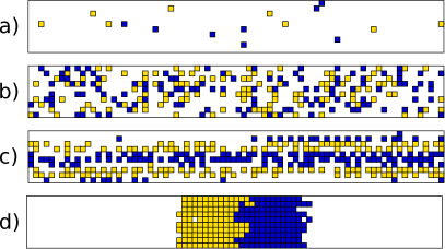
Figure 2: (Color online) Definition of states: a) Free flow, b) Disorder, c) Lanes, d) Gridlock.

III.2 Simulation Procedure

The simulations were done as follows: Initially, the $N=\rho WL$ particles are distributed randomly on the lattice. Then the simulation starts for different densities $\rho\in\{0.05,0.06,0.07,\ldots,1.00\}$ and for different coupling constants $k_{\text{D}}\in\{0.0,0.1,0.2,\ldots,7.5\}$. For each pair $(\rho,k_{\text{D}})$ of parameters the simulation was repeated at least 100 times. The simulation runs were stopped if one of the following conditions is fulfilled:

1. The flow $J$ averaged over the last 50 timesteps is lower than $\frac{1}{2WL}=5\times 10^{-4}$. This criterion indicates the formation of a gridlock.

2. The maximum and minimum value $\Phi_{\text{max}}$ and $\Phi_{\text{min}}$ of the order parameter $\Phi$ in the last 1000 timesteps fulfills the following condition

   $$\frac{\Phi_{\text{max}}-\Phi_{\text{min}}}{\Phi_{\text{max}}+\Phi_{\text{min}}}<0.1\,,$$ (14)

   which indicates the formation of lanes.

3. The number of timesteps exceeds the density dependent value $T_{\mathrm{max}}=20000\sqrt{\rho}$. This typically happens for disordered or free flow states.

If a simulation is stopped due to the second or third condition, the velocity $v$, flow $J$ and order parameter $\Phi$ are averaged over the last 1000 timesteps. Since the first condition means that the average number of particles which moved towards their desired direction is less than $\frac{1}{2}$, it indicates the occurrence of a gridlock. For a given set of parameters, the fraction of simulation runs which are aborted due to the first condition defines the jam probability $P_{\text{Jam}}$. Condition 2 indicates the occurrence of lanes. However, it does not contain any restrictions for the absolute value of the order parameter $\Phi$, because more than 99% of all values for $\Phi$ are anyway larger than $0.85$ given that $\Phi$ converges.

Finally, the last condition ensures that the computation time for a simulation run is finite. The value of $T_{\mathrm{max}}$ is based on the experience that lanes and gridlocks are formed much more quickly, if at all. The factor $\sqrt{\rho}$ takes into account that the system takes more time to evolve into a stationary state if the number of particles is increased. Using $\sqrt{\rho}$ instead of $\rho$ leads to a fast decrease in simulation time at low densities where the system does evolve neither into a jammed state nor a lane state.

III.3 Results

III.3.1 Jam Probability

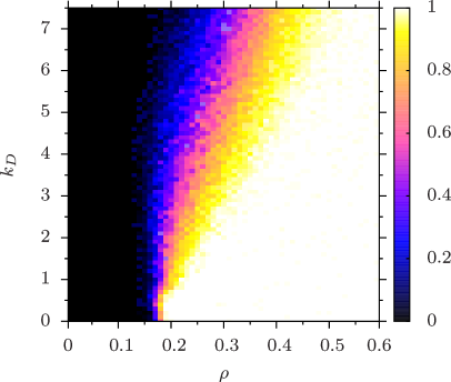
Figure 3: (Color online) Jam probability $P_{\mathrm{Jam}}$ as function of the density $\rho$ and the coupling constants $k_{\mathrm{A}}$ and $k_{\mathrm{D}}$. Left: $k_{\mathrm{D}}>0$, $k_{\mathrm{A}}=0$. Right: $k_{\mathrm{D}}=0$, $k_{\mathrm{A}}>0$.

As a first result one observes that in general the jam probability $P_{\text{jam}}$ increases both with an increasing density and a decreasing coupling constant $k_{\text{D}}$ and $k_{\text{A}}$, respectively (Fig. 3).

This result is not very surprising since an increasing density means a larger number of opposing particles which can block each other. Additionally, there is less space to avoid such collisions. An increasing $k_{\text{D}}$ means that it becomes more likely for a particle to follow another particle of the same kind and thus collisions of type-$A$ and type-$B$ particles are avoided. That the AFF prevents collisions is more obvious, because it prevents by definition particles from coming too close to opposing particles in the same row.

The simulations clearly indicate that the AFF is more capable to prevent jams compared to the DFF. If the AFF is turned off ($k_{A}=0$, Fig. 3 left) all simulations with a density larger than 0.5 evolve into a gridlock. Even for $\rho=0.2$ one has a non-vanishing jam probability. Anticipation leads to a vanishing jam probability for a sufficiently large coupling constant $k_{\text{A}}>3$ at almost every density.

III.3.2 Order Parameter

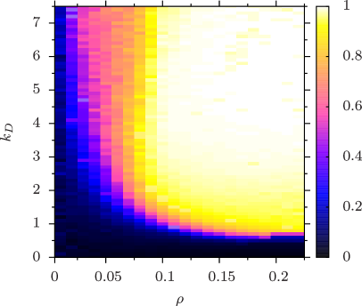
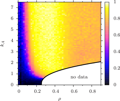
Figure 4: (Color online) Reduced order parameter $\tilde{\Phi}$ as function of the density $\rho$ and the coupling constants. Left: $k_{\mathrm{D}}>0$, $k_{\mathrm{A}}=0$. Right: $k_{\mathrm{D}}=0$, $k_{\mathrm{A}}>0$.

Now we consider only those simulation runs which are not aborted due to the detection of a gridlock. In general, the averaged reduced order parameter $\tilde{\Phi}$ becomes larger for increasing densities $\rho$ and coupling constant (see Fig. 4).

As expected, for $k_{\text{D}}=k_{\text{A}}=0$ the reduced order parameter is close to zero for all densities. The fact that it is slightly above zero can be explained by the increased number of sidesteps a particle has to perform if it has contact to a particle of different kind. These collisions happen more frequently if the number of type-$A$ and type-$B$ particles in a specific row is similar. The resulting sidesteps lead to a decreasing stability of homogeneous states.

By increasing the coupling constants the order parameter $\tilde{\Phi}$ shows a specific behavior which depends on the density. The dependence is qualitatively the same for lanes that are formed by the DFF and AFF, but for the latter there are more data for larger densities available due to a smaller jam probability. One can see that a certain minimal density is needed to reach an order parameter which is close to 1. The transition from a disordered state to a state with almost perfect lanes becomes sharper for increasing density. For densities $\rho>0.2$ the transition can only be observed at a few data points because most of the simulations evolve into a gridlock for small coupling constants. In particular there is no stable disordered state for large $\rho$ and the system evolves either in a jammed state or in a state with almost perfect lanes.

III.3.3 Dependence on the System Size

Since the behavior is quite sensitive to the size of the system, we want to discuss briefly the influence of the dimensions.

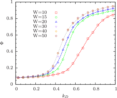
Figure 5: (Color online) Dependence of the order parameter on the system size at density $\rho=0.15$.

The results for the order parameter $\Phi$, which can be found in Fig. 5, show that $\Phi$ increases with increasing width $W$ of the corridor if the length $L$ remains constant. This increase seems to converge at a width of about $W=30$, since the value of the order parameter does not change if $W$ is increased further.

A similar scaling of the system length $L$ could not be performed due to the increasing jam probability in that case (cf. Fig. 6).

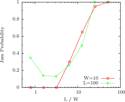
Figure 6: (Color online) Dependence of the jam probability on the system size ($\rho=0.2$, $k_{\mathrm{D}}=2$).

As a rough approximation one can say that $P_{\text{jam}}$ does only depend on the ratio $L/W$ and is monotonously increasing with this ratio. But this is only justified for smaller systems and $L/W>1$. For large values of $W$ one can observe that $P_{\text{jam}}$ is non-monotonic whereas $P_{\text{jam}}$ increases with increasing $W$.

IV Properties of the Lane State

IV.1 Distribution of Densities

In this Section we discuss how the particles distribute in the system after the formation of lanes. The data are taken after a simulation run was stopped due the lane condition (14) as described in Section III.2.

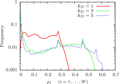
Figure 7: (Color online) Distribution of densities in the different rows. The global density is $\rho=0.15$, the bin size is 0.01.

Figure 7 shows the distribution of densities $\rho_{i}$ in the different rows $i\in\{1,\ldots,W\}$. If the particles were equally distributed over the system, one would expect a sharp peak in the distribution at the position of the global density $\rho$. This is for instance the case in a system without DFF, even if anticipation is included. But since the DFF implies an attractive interaction between particles, the number of rows which are not occupied as well as the number of rows with larger density grows. This can be observed in the distribution as a maximum at $\rho_{i}=0$ and a larger support for increasing coupling constant $k_{\text{D}}$. The latter means that the mobility of particles and thus the average velocity is reduced. This will be analyzed in more detail in Section IV.2.

Another feature of the distribution is the existence of characteristic lane densities which do neither depend on the coupling constant nor on the global density. This surprising result was tested for different coupling constants $k_{\text{D}}\in[1,7]$ and for different (global) densities $\rho\in[0.1,0.3]$. These lane densities become visible as peaks in the distribution at $\rho_{1}^{*}=0.28$, $\rho_{2}^{*}=0.46$ and $\rho_{3}^{*}=0.56$. The different peaks correspond to states with different number of lanes, i.e., $\rho_{j}^{*}$ corresponds to a configuration with $j+1$ lanes. Narrow lanes have a higher density than wide lanes. Note that the tendency of forming more lanes ($N_{\mathrm{lanes}}>2$) increases with increasing coupling constant $k_{D}$. Therefore, for small coupling constants (e.g., $k_{\mathrm{D}}=1$) only 2-lane configurations occur resulting in a single peak whereas for large coupling constants (e.g., $k_{\mathrm{D}}=5$) also 3- and 4-lane configurations occur resulting in three peaks.

Furthermore, under certain circumstances there are additional peaks in the distribution. At small densities and large coupling constants $k_{\text{D}}$ almost all particles of equal type are located in the same row. This causes additional density dependent peaks. For example at $\rho=0.1$ and a system of size $100\times 10$ there are 50 particles of each type and the maximal possible density in one row of the lane state is $\rho_{i}=0.5$. Therefore, if $k_{\text{D}}$ ist large, there is a peak at $\rho^{*}=0.5$ in the distribution. A similar effect can be found for large global densities. Then there can be an additional maximum beyond $\rho_{3}^{*}$ which can even have a larger value.

IV.2 Velocities

Since lane formation is a way of separating different types of particles which leads to less opposing traffic one would expect that lanes increase the mean velocity $v$ in the system, i.e., that $v(k_{\mathrm{A}})$ is monotonously increasing. However, this is only true for lanes which are formed due to the AFF, i.e., $v(k_{\mathrm{A}})$ is monotonously increasing nowak_lanes .

As one can see in Fig. 8, the dependence of $v$ on $k_{\text{D}}$ is not always monotonous.

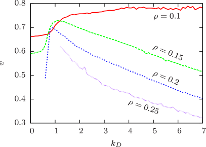
Figure 8: (Color online) Velocities in dependence of the coupling constant $k_{\text{D}}$. The data are gained by the simulation procedure described in Section III.2.

The DFF acts attracting on particles of the same type and thus the local densities in a row can be large, as seen in the previous section (cf. Fig. 7). This means in general a decrease of velocity, because particles are hindered by particles of the same kind. Thus there is a decrease in $v(k_{\text{D}})$. Note that a state with maximal velocity has not necessarily a maximal order parameter.

Note that not for all densities a maximum is present. For instance at $\rho=0.1$ the global density does not suffice to create a local density which is larger than 0.5. Hence, each particle has on average at least one empty cell in front and the velocity does not decrease. If the density is too large one has also no maximum because there are no data available for small $k_{D}$ due to a large jam probability, i.e., the curve $v(k_{\text{D}})$ starts at some $k_{\mathrm{D}}>0$ and can be monotonously decreasing in this case.

IV.3 Stability and Lifetime

In agreement with the observations in empirical studies zhang02 the general structure of lanes in the simulations fluctuates in time. The number of lanes changes due the vanishing of lanes or merging of neighbouring lanes to a broader one. In this section we will analyze this phenomenon. Previously, simulations were initialized in a disordered state and evolved into a lane state. Now we take the inverse approach, i.e., the simulations are started in a state where lanes already have formed and we wait until this structure is destroyed. The lifetime of lanes will serve as a measurement for their stability. Since the stability depends on the lane width we use different initial conditions with 2, 3 and 4 lanes. The simulation starts with one of these initial conditions and is stopped if either the number of timesteps exceeds $T_{\text{max}}=1.5\times 10^{5}$ or if the order parameter $\Phi$ falls below $\frac{1}{\sqrt{2}}$. The first condition is necessary to perform the simulation runs in an acceptable time. This might distort the result for states which have lifetimes of order $T_{\text{max}}$. However, $T_{\text{max}}=1.5\times 10^{5}$ corresponds to more than 10 hours in real time since one timestep corresponds to about $0.25$ seconds.

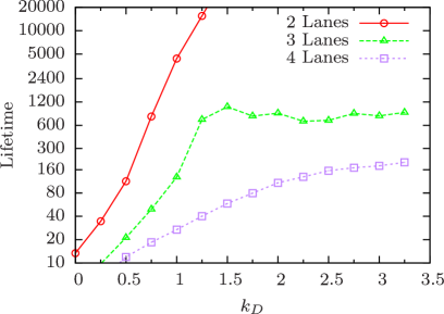
Figure 9: (Color online) Lifetime of lanes for different initial conditions for a density of $\rho=0.25$.

The results are shown in Fig. 9. The two-lane lifetime increases roughly exponentially with increasing $k_{\text{D}}$. It is not surprising that the stability is decreased if the number of lanes is increased because then the fraction of particles which are at the interface between two lanes becomes larger. The three-lane lifetime only increases up to a value of $k_{\text{D}}\approx 1.25$ where one can see a kink in the curve. For larger values of $k_{\text{D}}$, the lifetime stays almost constant at a value of about 1000 timesteps. Finally, the four-lane configuration has a lifetime which smoothly converges to a value of about 250.

Simulation with anticipation but without the DFF show a different behavior. The influence of the number of lanes on the lifetime is smaller. The two-lane configuration has still the largest lifetimes, but the difference in the stability of the three- and four-lane configuration becomes very small for increasing coupling constants. In all three cases the lifetime grows faster than exponential with $k_{A}$.

The fate of a system which has lost its stability depends on the density and the value of the coupling constant (cf. Fig. 3 and 4 from Section III). For large densities and a small coupling constant, the system evolves into a jam state. For small densities and a small coupling constant, the system evolves into a disordered state. If the coupling constant is large, i.e., at least large enough to prevent jams, the system can form lanes again. If the initial configuration consists of more than two lanes one can sometimes observe that the lanes are merging. In that case the final configuration consists of two lanes. Usually this happens only in systems with large coupling to the DFF, because then the attraction between two lanes with the same walking direction is strong. In most cases the order parameter $\Phi$ falls below $\frac{1}{\sqrt{2}}$, such that the simulation is aborted and the correct lifetime is taken. Anyway, sometimes it happens that lanes are merging without an appreciable decrease of $\Phi$ and thus the condition for stability is useless. The frequency of these incidents increases with increasing $k_{D}$ and make up to 50%. Fortunately, one can easily identify these cases in the data, because the lifetime of a 2-lane configuration is much larger and thus their is a huge gap (at least one magnitude) in the distribution of lifetimes. Hence, we only take into account the results below this gap.

V Open Boundary Conditions

V.1 Two Groups Passing Each Other

For this scenario we start the simulation with two groups of particles at the very left and the very right end of the system (cf. Fig. 10a). Each group contains 100 individuals of type $A$ and $B$, respectively. They walk in their desired walking direction until they reach the boundary of the system. There they are absorbed and removed from the system. The simulation ends when the flow becomes zero, i.e., if either all particles are removed or a gridlock is formed. The simulation was repeated 5000 times for each pair of parameters $(k_{\text{D}},k_{\text{A}})\in\{0,1,2,3,4\}^{2}$.

The first question is whether the groups are able to pass each other or not. If both dynamic floor field and anticipation is turned off, the system always evolves in a gridlock state. If $k_{D}$ becomes larger the jam probability is much reduced, e.g., for $k_{D}=2$ (but $k_{A}=0$) about 50% of simulation runs form a gridlock. For $k_{D}\geq 0$ and $k_{A}\geq 2$ no gridlocks were observed at all. As before we only take into account those simulation runs which did not end in a gridlock.

In order to quantify the tendency of collisions, we introduce a collision index $n_{c}$ as follows: A “collision” is defined as a pair of two neighboring cells, where the left one is occupied by a type-$A$ particle and the right one by a type-$B$ particle. Let $N_{\text{Col}}$ be the number of those pairs in the system. Then the collision index is defined as

$$n_{c}=2\frac{N_{\text{Col}}}{N}$$ (15)

where $N$ is the total number of particles.

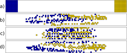
Figure 10: (Color online) Two groups walking past each other. a) Initial conditions. b)-d) Snapshot of the simulation at timestep 75. b) $k_{D}=2,k_{A}=0$, c) $k_{D}=0,k_{A}=2$, d) $k_{D}=k_{A}=2$.

One can observe that the dynamics shows qualitative differences depending on the choice of the coupling constants. Without anticipation it is strongly influenced by collisions between opposing particles (cf. Fig. 10b and 11). Even after most of the particles have already left the system there are almost always small groups of particles which form a jam that dissipates after longer time. Therefore, the collision index $n_{c}$ fades very slowly. Lanes can only be formed after both groups get in direct contact with each other, but they are less distinctive compared to those in the periodic system. This leads to a quite small order parameter.

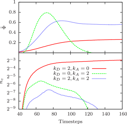
Figure 11: (Color online) Order parameter $\Phi$ and collision index $n_{c}$ from eqn. (15) versus time for two groups walking past each other.

With anticipation collisions are much less likely, but there are also difference in the dynamics depending on whether the DFF is turned on. If not, many thin lanes are formed during the contact (Fig. 10c). After the groups have passed each other these lanes are destroyed immediately. This can also be observed in terms of the order parameter in Fig. 11. Probably the most realistic results were attained by a combination of AFF and DFF. The tendency of collisions is reduced further. Lanes can be seen clearly even if the order parameter is a bit reduced compared to the system with AFF only. This can be explained by lanes which are often not parallel to the walking direction (Fig. 10d). Their number is much decreased and one usually observes 2 or 3 lanes. The lane structure is kept after the groups have passed each other.

V.2 Random Insertion of Particles

Now the particles are inserted and removed dynamically with a certain insertion probability $\beta_{\text{in}}=\beta$ on each cell next to the boundaries. At the left (right) boundary only type-$A$ (type-$B$) particles are inserted. Like in the previous section, the removal of particles will always happen, i.e., with probability $\beta_{\text{out}}=1$ at the left and right boundary, respectively. The left boundary absorbs only type-$B$ particles whereas the right boundary absorbs only type-$A$ particles.

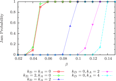
Figure 12: (Color online) Jam probability at timestep 20000 for open boundary conditions.

Fig. 12 shows the probability that the system evolves into a gridlock before timestep 20000. It turns out that the avoidance of jams is much harder as in the periodic system. The DFF does not help very much to prevent jams but astonishingly it rather supports the formation of a jam.

Anticipation helps much to avoid gridlocks and even for an insertion probability of $\beta=0.12$ gridlocks can be avoided. We find a linear dependence between $\beta$ and $\rho$. The constant of proportionality depends slightly on the exact value of the coupling constants and ranges from 2.5 to 2.8. This means that the maximal density in the system without forming a gridlock is about $\rho=0.34$.

Before gridlocks are formed, the system usually forms lanes for sufficiently large coupling constants. The order parameter is lower than in the periodic case, but comparable to the findings in the previous section (Fig. 11).

It is not surprising that systems with open boundary conditions show a slightly different gridlock behaviour from that with periodic boundaries. In the periodic case the flow in a system near a gridlock becomes very small. In contrast, in the open system still additional particles are fed into the system. Due to particles moving up ”from behind” the chances for the gridlock to resolve are strongly reduced.

VI Conclusions

We have studied the phenomenon of lane formation in a cellular automaton model for pedestrian dynamics. In contrast to previous studies, we have obtained for the first time quantitative results. This was possible by introducing an order parameter which has been adapted from the analysis of colloidal suspensions. It has been shown that this order parameter is suitable for the detection of lanes, at least for the simple scenario of a straight corridor considered here.

It is found that at least four different states can be distinguished, namely free flow, disordered flow, lane formation and gridlock. Using the order parameter we have mapped out the parameter range of the model for which lane formation is possible. Also other quantities like density and velocity show a very characteristic behavior in these scenarios.

Most models for pedestrian dynamics show a strong tendency towards gridlock which appear for large densities. This is rather unrealistic and was not observed in experimental studies. A model extension which includes an anticipation mechanism was found to show a more realistic behavior by suppressing the formation of gridlocks, at least in the case of periodic boundary conditions.

Although we have focussed on the floor field model and its variants we want to emphasized that the techniques developed here can also be applied to most other models.

References

- (1) A. Schadschneider, W. Klingsch, H. Klüpfel, T. Kretz, C. Rogsch, and A. Seyfried, in Encyclopedia of Complexity and Systems Science, edited by R. A. Meyers (Springer, 2009) pp. 3142–3176
- (2) T. Mullin, Science 295, 1851 (2002)
- (3) B. Schmittmann and R. K. P. Zia, Phys. Rep. 301, 45 (1998)
- (4) K. R. Sütterlin, A. Wysocki, A. V. Ivlev, C. Räth, H. M. Thomas, M. Rubin-Zuzic, W. J. Goedheer, V. E. Fortov, A. M. Lipaev, V. I. Molotkov, O. F. Petrov, G. E. Morfill, and H. Löwen, Phys. Rev. Lett. 102, 085003 (2009)
- (5) R. R. Netz, Europhys. Lett. 63, 616 (2003)
- (6) J. Dzubiella, G. P. Hoffmann, and H. Löwen, Phys. Rev. E 65, 021402 (2002)
- (7) M. E. Leunissen, C. G. Christova, A.-P. Hynninen, P. Royall, A. I. Campbell, A. Imhof, M. Dijkstra, R. van Roij, and A. van Blaaderen, Nature 437, 235 (2005)
- (8) M. Rex and H. Löwen, Phys. Rev. E 75, 051402 (2007)
- (9) M. Rex and H. Löwen, Eur. Phys. J. E 26, 143 (2008)
- (10) T. Vissers, A. Wysocki, M. Rex, H. Löwen, C.P. Royall, A. Imhof and A. van Blaaderen, Soft Matter 7, 2352–2356 (2011)
- (11) F. Navin and R. Wheeler, Traffic Engineering 39, 30 (1969)
- (12) S. P. Hoogendoorn and W. Daamen, in Traffic and Granular Flow 2003 (Springer, 2005) pp. 373–382
- (13) T. Kretz, A. Grünebohm, M. Kaufman, F. Mazur, and M. Schreckenberg, J. Stat. Mech., P10001(2006)
- (14) Y. Suma, D. Yanagisawa, and K. Nishinari, Physica A 391, 248 (2012)
- (15) M. Isobe, T. Adachi, and T. Nagatani, Physica A 336, 638 (2004)
- (16) V. J. Blue and J. L. Adler, Transp. Res. Rec. 1678, 135 (1999)
- (17) F. Weifeng, Y. Lizhong, and F. Weicheng, Physica A 321, 633 (2003)
- (18) W. G. Weng, T. Chen, H. Y. Yuan, and W. C. Fan, Phys. Rev. E 74, 036102 (2006)
- (19) Y. F. Yu and W. G. Song, Phys. Rev. E 75, 046112 (2007)
- (20) C. Burstedde, K. Klauck, A. Schadschneider, and J. Zittartz, Physica A 295, 507 (2001)
- (21) M. Muramatsu, T. Irie, and T. Nagatani, Physica A 267, 487 (1999)
- (22) Y. Tajima, K. Takimoto, and T. Nagatani, Physica A 313, 709 (2002)
- (23) K. Takimoto, Y. Tajima, and T. Nagatani, Physica A 308, 460 (2002)
- (24) K. Hua, S. Tao, L. Xing-Li, and D. Shi-Qiang, Chin. Phys. Lett. 25, 1498 (2008)
- (25) T. Nagatani, Phys. Lett. A 373, 2917 (2009)
- (26) T. Kretz, M. Kaufman, and M. Schreckenberg, Lecture Notes in Computer Science 5191, 555 (2008)
- (27) W. Weng, S. Shen, H. Yuan, and W. Fan, Physica A 375, 668 (2007)
- (28) W. J. Yu, R. Chen, L. Y. Dong, and S. Q. Dai, Phys. Rev. E 72, 026112 (2005)
- (29) D. Helbing, P. Molnar, I. J. Farkas, and K. Bolay, Environment and Planning B: Planning and Design 28, 361 (2001)
- (30) Y. Jiang, T. Xiong, S. Wong, C. Shu, M. Zhang, P. Zhang, and W. Lam, Acta Mathematica Scientia 29, 1541 (2009)
- (31) T. Xiong, P. Zhang, S. Wong, C.-W. Shu, and M. Zhang, “A macroscopic approach to the lane formation phenomenon in pedestrian counter flow,” (2010), http://www.dam.brown.edu/scicomp/reports/2010-34
- (32) A. Schadschneider, A. Kirchner, and K. Nishinari, Lecture Notes in Computer Science 2493, 239 (2002)
- (33) R. Nagai, M. Fukamachi, and T. Nagatani, Physica A 358, 516 (2005)
- (34) J. Zhang, W. Klingsch, A. Schadschneider, and A. Seyfried, “Ordering in bidirectional pedestrian flows and its influence on the fundamental diagram,” (2012)
- (35) A. Kirchner and A. Schadschneider, Physica A 312, 260 (2002)
- (36) A. Kirchner, K. Nishinari, and A. Schadschneider, Phys. Rev. E 67, 056122 (2003)
- (37) J. Tanimoto, A. Hagishima, and Y. Tanaka, Physica A 389, 5611–5618 (2010)
- (38) X.P. Zheng, and Y. Cheng, Physica A 390, 1042–1050 (2011)
- (39) Q.-Y. Hao,R. Jiang,M.-B. Hu,B. Jia, and Q.-S. Wu, Phys. Rev. E 84, 036107 (2011)
- (40) E. Kirik, T. Yurgel’yan, and D. Krouglov, in Proceedings of the 2007 Summer Computer Simulation Conference, edited by G. A. Wainer (2007) p. 1363
- (41) K. Hua, L. Xing-Li, W. Yan-Fang, S. Tao, and D. Shi-Qiang, Chin. Phys. B 19, 070517 (2010)
- (42) J. Dijkstra, A. Jessurun, and H. Timmermans, in Pedestrian and Evacuation Dynamics (Springer, 2002) pp. 173–181
- (43) A. Schadschneider, A. Kirchner, and K. Nishinari, Applied Bionics and Biomechanics 1, 11 (2003)
- (44) S. Nowak, A cellular automaton model for lane formation in pedestrian counterflow, Master’s thesis, Universität zu Köln. (2011)
- (45) K. Yamori, Psychological Review 105, 530 (1998)