Identifiability and Unmixing of Latent Parse Trees

Abstract

This paper explores unsupervised learning of parsing models along two directions. First, which models are identifiable from infinite data? We use a general technique for numerically checking identifiability based on the rank of a Jacobian matrix, and apply it to several standard constituency and dependency parsing models. Second, for identifiable models, how do we estimate the parameters efficiently? EM suffers from local optima, while recent work using spectral methods [1] cannot be directly applied since the topology of the parse tree varies across sentences. We develop a strategy, unmixing, which deals with this additional complexity for restricted classes of parsing models.

1 Introduction

Generative parsing models, which define joint distributions over sentences and their parse trees, are one of the core techniques in computational linguistics. We are interested in the unsupervised learning of these models [2, 3, 4, 5, 6], where the goal is to estimate the model parameters given only examples of sentences. Unsupervised learning can fail for a number of reasons [7]: model misspecification, non-identifiability, estimation error, and computation error. In this paper, we delve into two of these issues: identifiability and computation. In doing so, we confront a central challenge of parsing models—that the topology of the parse tree is unobserved and varies across sentences. This is in contrast to standard phylogenetic models [8] and other latent tree models for which there is a single fixed global tree across all examples [9].

A model is identifiable if there is enough information in the data to pinpoint the parameters (up to some trivial equivalence class); establishing the identifiability of a model is often a highly non-trivial task. A classic result of Kruskal [10] has been employed to prove the identifiability of a wide class of latent variable models, including hidden Markov models and certain restricted mixtures of latent tree models [11, 12, 13]. However, these techniques cannot be directly applied to parsing models since the tree topology varies over an exponential set of possible topologies. Instead, we turn to techniques from algebraic geometry [14, 15, 16, 17]; we show that a simple numerical procedure can be used to check identifiability for a wide class of models in NLP. Using this tool, we discover that probabilistic context-free grammars (PCFGs) are non-identifiable, but that simpler PCFG variants and dependency models are identifiable.

The most common way to estimate unsupervised parsing models is by using local techniques such as EM [18] or MCMC sampling [19], but these methods can suffer from local optima and slow mixing. Meanwhile, recent work [20, 21, 22, 23, 1] has shown that spectral methods can be used to estimate mixture models and HMMs with provable guarantees. These techniques express low-order moments of the observable distribution as a product of matrix parameters and use eigenvalue decomposition to recover these matrices. However, these methods are not directly applicable to parsing models because the tree topology again varies non-trivially. To address this, we propose a new technique, unmixing. The main idea is to express moments of the observable distribution as a mixture over the possible topologies. For restricted parsing models, the moments for a fixed tree structure can be “unmixed”, thereby reducing the problem to one with a fixed topology, which can be tackled using standard techniques [1]. Importantly, our unmixing technique does not require the training sentences be annotated with the tree topologies a priori, in contrast to recent extensions of [21] to learning PCFGs [24] and dependency trees [25, 26], which work on a fixed topology.

2 Notation

For a positive integer $n$, define $[n]\stackrel{{\scriptstyle\rm def}}{{=}}\{1,\dots,n\}$ and $\left\langle n\right\rangle=\{e_{1},\dots,e_{n}\}$, where $e_{i}$ is the vector which is 1 in component $i$ and 0 elsewhere. For integers $a,b\in[n]$, let $a\otimes_{n}b=(a-1)n+b\in[n^{2}]$ be the integer encoding of the pair $(a,b)$. For a pair of matrices, $A,B\in\mathbb{R}^{m\times n}$, define the columnwise tensor product $A\otimes^{\text{\sc c}}B\in\mathbb{R}^{m^{2}\times n}$ to be such that $(A\otimes^{\text{\sc c}}B)_{(i_{1}\otimes_{m}i_{2})j}=A_{i_{1}j}B_{i_{2}j}$. For a matrix $A\in\mathbb{R}^{m\times n}$, let $A^{\dagger}$ denote the Moore-Penrose pseudoinverse.

3 Parsing models

A sentence is a sequence of $L$ words, $\mathbf{x}=(x_{1},\dots,x_{L})$, where each word $x_{i}\in\left\langle d\right\rangle$ is one of $d$ possible word types. A (generative) parsing model defines a joint distribution $\mathbb{P}_{\theta}(\mathbf{x},z)$ over a sentence $\mathbf{x}$ and its parse tree $z$ (to be made precise later), where $\theta$ are the model parameters (a collection of multinomials). Each parse tree $z$ has a topology $\operatorname*{Topology}(z)\in\operatorname*{Topologies}$, which is both unobserved and varying across sentences. The learning problem is to recover $\theta$ given only samples of $\mathbf{x}$.

Two important classes of models of natural language syntax are constituency models, which represent a hierarchical grouping and labeling of the phrases of a sentence (e.g., Figure 1(a)), and dependency models, which represent pairwise relationships between the words of a sentence (e.g., Figure 1(b)).

Figure 1: The two constituency trees and seven dependency trees over $L=3$ words, $x_{1},x_{2},x_{3}$. (a) A constituency tree consists of a hierarchical grouping of the words with a latent state $z_{v}$ for each node $v$. (b) A dependency tree consists of a collection of directed edges between the words. In both cases, we have labeled each edge from $i$ to $j$ with the parameters used to generate the state of node $j$ given $i$.

3.1 Constituency models

A constituency tree $z=(V,s)$ consists of a set of nodes $V$ and a collection of hidden states $s=\{s_{v}\}_{v\in V}$. Each state $s_{v}\in\left\langle k\right\rangle$ represents one of $k$ possible syntactic categories. Each node $v$ has the form ${[i:j]}$ for $0\leq i<j\leq L$ corresponding to the phrase between positions $i$ and $j$ of the sentence. These nodes form a binary tree as follows: the root node is ${[0:L]}\in V$, and for each node ${[i:j]}\in V$ with $j-i>1$, there exists a unique $m$ with $i<m<j$ defining the two children nodes ${[i:m]}\in V$ and ${[m:j]}\in V$. Let $\operatorname*{Topology}(z)$ be an integer encoding of $V$.

PCFG.

Perhaps the most well-known constituency parsing model is the probabilistic context-free grammar (PCFG). The parameters of a PCFG are $\theta=(\pi,B,O)$, where $\pi\in\mathbb{R}^{k}$ specifies the initial state distribution, $B\in\mathbb{R}^{k^{2}\times k}$ specifies the binary production distributions, and $O\in\mathbb{R}^{d\times k}$ specifies the emission distributions.

A PCFG corresponds to the following generative process (see Figure 1(a) for an example): choose a topology $\operatorname*{Topology}(z)$ uniformly at random; generate the state of the root node using $\pi$; recursively generate pairs of children states given their parents using $B$; and finally generate words $x_{i}$ given their parents using $O$. This generative process defines a joint probability over a sentence $\mathbf{x}$ and a parse tree $z$:

$$\mathbb{P}_{\theta}(\mathbf{x},z)=|\operatorname*{Topologies}|^{-1}\pi^{\top}s_{{[0:L]}}\prod_{{[i:m]},{[m:j]}\in V}(s_{{[i:m]}}\otimes_{k}s_{{[m:j]}})^{\top}Bs_{{[i:j]}}\prod_{i=1}^{L}x_{i}^{\top}Os_{{[i-1:i]}},$$ (1)

We will also consider two variants of the PCFG with additional restrictions:

PCFG-I.

The left and right children states are generated independently—that is, we have the following factorization: $B=T_{1}\otimes^{\text{\sc c}}T_{2}$ for some $T_{1},T_{2}\in\mathbb{R}^{k\times k}$.

PCFG-IE.

The left and the right productions are independent and equal: $B=T\otimes^{\text{\sc c}}T$.

3.2 Dependency tree models

In contrast to constituency trees, which posit internal nodes with latent states, dependency trees connect the words directly. A dependency tree $z$ is a set of directed edges $(i,j)$, where $i,j\in[L]$ are distinct positions in the sentence. Let $\operatorname*{Root}(z)$ denote the position of the root node of $z$. We consider only projective dependency trees [27]: $z$ is projective if for every path from $i$ to $j$ to $k$ in $z$, we have that $j$ and $k$ are on the same side of $i$ (that is, $j-i$ and $k-i$ have the same sign). Let $\operatorname*{Topology}(z)$ be an integer encoding of $z$.

DEP-I.

We consider the simple dependency model of [4]. The parameters of this model are $\theta=(\pi,A_{\swarrow},A_{\searrow})$, where $\pi\in\mathbb{R}^{d}$ is the initial word distribution and $A_{\swarrow},A_{\searrow}\in\mathbb{R}^{d\times d}$ are the left and right argument distributions. The generative process is as follows: choose a topology $\operatorname*{Topology}(z)$ uniformly at random, generate the root word using $\pi$, and recursively generate argument words to the left to the right given the parent word using $A_{\swarrow}$ and $A_{\searrow}$, respectively. The corresponding joint probability distribution is as follows:

$$\mathbb{P}_{\theta}(\mathbf{x},z)=|\operatorname*{Topologies}|^{-1}\pi^{\top}x_{\operatorname*{Root}(z)}\prod_{(i,j)\in z}x_{j}^{\top}A_{\operatorname*{dir}(i,j)}x_{i},$$ (2)

where $\operatorname*{dir}(i,j)=\,\swarrow$ if $j<i$ and $\searrow$ if $j>i$.

We also consider the following two variants:

DEP-IE.

The left and right argument distributions are equal: $A=A_{\swarrow}=A_{\searrow}$.

DEP-IES.

$A=A_{\swarrow}=A_{\searrow}$ and $\pi$ is the stationary distribution of $A$ (that is, $\pi=A\pi$).

4 Identifiability

Our goal is to estimate model parameters ${\theta_{0}}\in\Theta$ given only access to sentences $\mathbf{x}\sim\mathbb{P}_{{\theta_{0}}}$. Specifically, suppose we have an observation function $\phi(\mathbf{x})\in\mathbb{R}^{m}$, which is the only lens through which an algorithm can view the data. We ask a basic question: in the limit of infinite data, is it information-theoretically possible to identify ${\theta_{0}}$ from the observed moments $\mu({\theta_{0}})\stackrel{{\scriptstyle\rm def}}{{=}}{\mathbb{E}}_{{\theta_{0}}}[\phi(\mathbf{x})]$?

To be more precise, define the equivalence class of ${\theta_{0}}$ to be the set of parameters $\theta$ that yield the same observed moments:

$$\mathcal{S}_{\Theta}({\theta_{0}}) =\{\theta\in\Theta:\mu(\theta)=\mu({\theta_{0}})\}.$$ (3)

It is impossible for an algorithm to distinguish among the elements of $\mathcal{S}_{\Theta}({\theta_{0}})$. Therefore, one might want to ensure that $|\mathcal{S}_{\Theta}({\theta_{0}})|=1$ for all ${\theta_{0}}\in\Theta$. However, this requirement is too strong for two reasons. First, models often have natural symmetries—e.g., the $k$ states of any PCFG can be permuted without changing $\mu(\theta)$, so $|\mathcal{S}_{\Theta}({\theta_{0}})|\geq k!$. Second, $|\mathcal{S}_{\Theta}({\theta_{0}})|=\infty$ for some pathological ${\theta_{0}}$’s—e.g., PCFGs where all states have the same emission distribution $O$ are indistinguishable regardless of the production distributions $B$. The following definition of identifiability accommodates these two exceptional cases:

Definition 1 (Identifiability).

A model family with parameter space $\Theta$ is (globally) identifiable from $\phi$ if there exists a measure zero set $\mathcal{E}$ such that $|\mathcal{S}_{\Theta}({\theta_{0}})|$ is finite for every ${\theta_{0}}\in\Theta\backslash\mathcal{E}$. It is locally identifiable from $\phi$ if there exists a measure zero set $\mathcal{E}$ such that, for every ${\theta_{0}}\in\Theta\backslash\mathcal{E}$, there exists an open neighborhood $N({\theta_{0}})$ around ${\theta_{0}}$ such that $\mathcal{S}_{\Theta}({\theta_{0}})\cap N({\theta_{0}})=\{{\theta_{0}}\}$.

Example of non-identifiability.

Consider the DEP-IE model with $L=2$ with the full observation function $\phi(\mathbf{x})=x_{1}\otimes x_{2}$. The corresponding observed moments are $\mu(\theta)=0.5A\operatorname*{diag}(\pi)+0.5\operatorname*{diag}(\pi)A^{\top}$. Note that $A\operatorname*{diag}(\pi)$ is an arbitrary $d\times d$ matrix whose entries sum to 1, which has $d^{2}-1$ degrees of freedom, whereas $\mu(\theta)$ is a symmetric matrix whose entries sum to 1, which has $\binom{d+1}{2}-1$ degrees of freedom. Therefore, $\mathcal{S}_{\Theta}(\theta)$ has dimension $\binom{d}{2}$ and therefore the model is non-identifiable.

Parameter counting.

It is important to compute the degrees of freedom correctly—simple parameter counting is insufficient. For example, consider the PCFG-IE model with $L=2$. The observed moments with respect to $\phi(\mathbf{x})=x_{1}\otimes x_{2}$ is a $d\times d$ matrix, which places $d^{2}$ constraints on the $k^{2}+(d-1)k$ parameters. When $d\geq 2k$, there are more constraints than parameters, but the PCFG-IE model with $L=2$ is actually non-identifiable (as we will see later). The issue here is that the number of constraints does not reveal the fact that some of these constraints are redundant.

4.1 Observation functions

An observation function $\phi(\mathbf{x})$ and its associated observed moments $\mu({\theta_{0}})=\mathbb{E}_{{\theta_{0}}}[\phi(\mathbf{x})]$ reveals aspects of the distribution $\mathbb{P}_{{\theta_{0}}}(\mathbf{x})$. For example, $\phi(\mathbf{x})=x_{1}$ would only reveal the marginal distribution of the first word, whereas $\phi(\mathbf{x})=x_{1}\otimes\cdots\otimes x_{L}$ reveals the entire distribution of $\mathbf{x}$. There is a tradeoff: Higher-order moments provide more information, but are harder to estimate reliably given finite data, and are also computationally more expensive. In this paper, we consider the following intermediate moments:

$$\phi_{{12}}(\mathbf{x}) \stackrel{{\scriptstyle\rm def}}{{=}}x_{1}\otimes x_{2} \phi_{{**}}(\mathbf{x}) \stackrel{{\scriptstyle\rm def}}{{=}}\bigl{(}x_{i}\otimes x_{j}:i,j\in[L]\bigr{)}$$

$$\phi_{{123}}(\mathbf{x}) \stackrel{{\scriptstyle\rm def}}{{=}}x_{1}\otimes x_{2}\otimes x_{3} \phi_{{***}}(\mathbf{x}) \stackrel{{\scriptstyle\rm def}}{{=}}\bigl{(}x_{i}\otimes x_{j}\otimes x_{k}:i,j,k\in[L]\bigr{)}$$

$$\phi_{{123\eta}}(\mathbf{x}) \stackrel{{\scriptstyle\rm def}}{{=}}(x_{1}\otimes x_{2})(\eta^{\top}x_{3}) \phi_{{***\eta}}(\mathbf{x}) \stackrel{{\scriptstyle\rm def}}{{=}}\bigl{(}(x_{i}\otimes x_{j})(\eta^{\top}x_{k}):i,j,k\in[L]\bigr{)}$$

$$\phi_{\operatorname{all}}(\mathbf{x}) \stackrel{{\scriptstyle\rm def}}{{=}}x_{1}\otimes\cdots\otimes x_{L}$$

Above, $\eta\in\mathbb{R}^{d}$ denotes a unit vector in $\mathbb{R}^{d}$ (e.g., $e_{1}$) which picks out a linear combination of matrix slices from a third-order $d\times d\times d$ tensor.

4.2 Automatically checking identifiability

One immediate goal is to determine which models in Section 3 are identifiable from which of the observed moments (Section 4.1). A powerful analytic tool that has been succesfully applied in previous work is Kruskal’s theorem [10, 11], but (i) it is does not immediately apply to models with random topologies, and (ii) only gives sufficient conditions for identifiability, and cannot be used to determine non-identifiability. Furthermore, since it is common practice to explore many different models for a given problem in rapid succession, we would like to check identifiability quickly and reliably. In this section, we develop an automatic procedure to do this.

To establish identifiability, let us examine the algebraic structure of $\mathcal{S}_{\Theta}({\theta_{0}})$ for ${\theta_{0}}\in\Theta$, where we assume that the parameter space $\Theta$ is an open subset of $[0,1]^{n}$. Recall that $\mathcal{S}_{\Theta}({\theta_{0}})$ is defined by the moment constraints $\mu(\theta)=\mu({\theta_{0}})$. We can write these constraints as $h_{\theta_{0}}(\theta)=0$, where

$$h_{\theta_{0}}(\theta)\stackrel{{\scriptstyle\rm def}}{{=}}\mu(\theta)-\mu({\theta_{0}})$$

is a vector of $m$ polynomials in $\theta$.

Let us now compute the number of degrees of freedom of $h_{\theta_{0}}$ around ${\theta_{0}}$. The key quantity is $J(\theta)\in\mathbb{R}^{m\times n}$, the Jacobian of $h_{{\theta_{0}}}$ at $\theta$ (note that the Jacobian of $h_{\theta_{0}}$ does not depend on ${\theta_{0}}$; it is precisely the Jacobian of $\mu$). This Jacobian criterion is well-established in algebraic geometry, and has been adopted in the statistical literature for testing model identifiability and other related properties [14, 15, 16, 17].

Intuitively, each row of $J({\theta_{0}})$ corresponds to a direction of a constraint violation, and thus the row space of $J({\theta_{0}})$ corresponds to all directions that would take us outside the equivalence class $\mathcal{S}_{\Theta}({\theta_{0}})$. If $J({\theta_{0}})$ has less than rank $n$, then there is a direction orthogonal to all the rows along which we can move and still satisfy all the constraints—in other words, $|\mathcal{S}_{\Theta}({\theta_{0}})|$ is infinite, and therefore the model is non-identifiable. This intuition leads to the following algorithm:

$\operatorname*{\text{\sc CheckIdentifiability}}$: $-$1. Choose a point ${\tilde{\theta}}\in\Theta$ uniformly at random. $-$2. Compute the Jacobian matrix $J({\tilde{\theta}})$. $-$3. Return “yes” if the rank of $J({\tilde{\theta}})=n$ and “no” otherwise.

The following theorem asserts the correctness of $\operatorname*{\text{\sc CheckIdentifiability}}$. It is largely based on techniques in [16], although we have not seen it explicitly stated in this form.

Theorem 1 (Correctness of $\operatorname*{\text{\sc CheckIdentifiability}}$).

Assume the parameter space $\Theta$ is a non-empty open connected subset of $[0,1]^{n}$; and the observed moments $\mu\colon\mathbb{R}^{n}\to\mathbb{R}^{m}$, with respect to observation function $\phi$, is a polynomial map. Then with probability 1, $\operatorname*{\text{\sc CheckIdentifiability}}$ returns “yes” iff the model family is locally identifiable from $\phi$. Moreover, if it returns “yes”, then there exists $\mathcal{E}\subset\Theta$ of measure zero such that the model family with parameter space $\Theta\setminus\mathcal{E}$ is identifiable from $\phi$.

The proof of Theorem 1 is given in Appendix A.

4.3 Implementation of $\operatorname*{\text{\sc CheckIdentifiability}}$

Computing the Jacobian.

The rows of $J$ correspond to $\partial\mathbb{E}_{\theta}[\phi_{j}(\mathbf{x})]/\partial\theta$ and can be computed efficiently by adapting dynamic programs used in the E-step of an EM algorithm for parsing models. There are two main differences: (i) we must sum over possible values of $\mathbf{x}$ in addition to $z$, and (ii) we are not computing moments, but rather gradients thereof. Specifically, we adapt the CKY algorithm for constituency models and the algorithm of [27] for dependency models. See Appendix C.1 for more details.

Numerical issues.

Because we implemented $\operatorname*{\text{\sc CheckIdentifiability}}$ on a finite precision machine, the results are subject to numerical precision errors. However, we verified that our numerical results are consistent with various analytically-derived identifiability results (e.g., from [11]).

4.4 Identifiability of constituency and dependency tree models

We checked the identifiability status of various constituency and dependency tree models using our implementation of $\operatorname*{\text{\sc CheckIdentifiability}}$. We focus on the regime where $d\geq k$ for PCFGs; additional results for $d<k$ are given in Appendix B.

Model $\backslash$ Observation function	$\phi_{12}$	$\phi_{**}$	$\phi_{123e_{1}}$	$\phi_{123}$	$\phi_{***e_{1}}$	$\phi_{***}$
PCFG	No, even from $\phi_{\operatorname{all}}$ for $L\in\{3,4,5\}$
PCFG-I / PCFG-IE	No	Yes iff $L\geq 4$	Yes iff $L\geq 3$
DEP-I	No	Yes iff $L\geq 3$
DEP-IE / DEP-IES	Yes iff $L\geq 3$

Figure 2: Local identifiability of parsing models. These findings are given by $\operatorname*{\text{\sc CheckIdentifiability}}$ have the semantics from Theorem 1. These were checked for $d\in\{2,3,\dotsc,8\}$, $k\in\{2,\dotsc,d\}$ (applies only for PCFG models), $L\in\{2,3,\dotsc,9\}$.

The results are reported in Figure 2. First, we found that the PCFG is not identifiable from $\phi_{\operatorname{all}}$ (and therefore not identifiable from any $\phi$) for $L\in\{3,4,5\}$; we believe that the same holds for all $L$. This negative result motivates exploring restricted subclasses of PCFGs, such as PCFG-I and PCFG-IE, which factorize the binary productions. For these classes, we found that the sentence length $L$ and choice of observation function can influence identifiability: Both models are identifiable for large enough $L$ (e.g., $L\geq 3$) and with a sufficiently rich observation function (e.g., $\phi_{123\eta}$).

The dependency models, DEP-I and DEP-IE, were all found to be identifiable for $L\geq 3$ from second-order moments $\phi_{**}$. The conditions for identifiability are less stringent than their constituency counterparts (PCFG-I and PCFG-IE), which is natural since dependency models are simpler without the latent states. Note that in all identifiable models, second-order moments suffice to determine the distribution—this is good news because low-order moments are easier to estimate.

5 Unmixing algorithms

Having established which parsing models are identifiable, we now turn to parameter estimation for these models. We will consider algorithms based on moment matching—those that try to find a $\theta$ satisfying $\mu(\theta)=u$ for some $u$. Typically, $u$ is an empirical estimate of $\mu({\theta_{0}})=\mathbb{E}_{{\theta_{0}}}[\phi(\mathbf{x})]$ based on samples $\mathbf{x}\sim\mathbb{P}_{{\theta_{0}}}$.

In general, solving $\mu(\theta)=u$ corresponds to finding solutions to systems of multivariate polynomials, which is NP-hard [28]. However, $\mu(\theta)$ often has additional structure which we can exploit. For instance, for an HMM, the sliced third-order moments $\mu_{123\eta}(\theta)$ can be written as a product of parameter matrices in $\theta$, and each matrix can be recovered by decomposing the product [1].

For parsing models, the challenge is that the topology is random, so the moments is not a single product, but a mixture over products. To deal with this complication, we propose a new technique, which we call unmixing: We “unmix” the products from the mixtures, essentially reducing the problem to one with a fixed topology.

We will first present the general idea of unmixing (Section 5.1) and then apply it to the PCFG-IE model (Section 5.2) and the DEP-IES model (Section 5.3).

5.1 General case

We assume the observation function $\phi(\mathbf{x})$ consists of a collection of observation matrices $\{\phi_{o}(\mathbf{x})\}_{o\in\mathcal{O}}$ (e.g., for $o=(i,j)$, $\phi_{o}(\mathbf{x})=x_{i}\otimes x_{j}$). Given an observation matrix $\phi_{o}(\mathbf{x})$ and a topology $t\in\operatorname*{Topologies}$, consider the mapping that computes the observed moment conditioned on that topology: $\Psi_{o,t}(\theta)={\mathbb{E}}_{\theta}[\phi_{o}(\mathbf{x})\mid\operatorname*{Topology}=t]$. As we range $o$ over $\mathcal{O}$ and $t$ over $\operatorname*{Topologies}$, we will enounter a finite number of such mappings. We call these mappings compound parameters, denoted $\{\Psi_{p}\}_{p\in\mathcal{P}}$.

Now write the observed moments as a weighted sum:

$$\mu_{o}(\theta) =\sum_{p\in\mathcal{P}}\underbrace{\mathbb{P}(\Psi_{o,\operatorname*{Topology}}=\Psi_{p})}_{\stackrel{{\scriptstyle\rm def}}{{=}}M_{op}}\Psi_{p}\quad\text{for all $o\in\mathcal{O}$},$$ (4)

where we have defined $M_{op}$ to be the probability mass over tree topologies that yield compound parameter $\Psi_{p}$. We let $\{M_{op}\}_{o\in\mathcal{O},p\in\mathcal{P}}$ be the mixing matrix. Note that (4) defines a system of equations $\mu=M\Psi$, where the variables are the compound parameters and the constraints are the observed moments. In a sense, we have replaced the original system of polynomial equations (in $\theta$) with a system of linear equations (in $\Psi$).

The key to the utility of this technique is that the number of compound parameters can be polynomial in $L$ even when the number of possible topologies is exponential in $L$. Previous analytic techniques [13] based on Kruskal’s theorem [10] cannot be applied here because the possible topologies are too many and too varied.

Note that the mixing equation $\mu=M\Psi$ holds for each sentence length $L$, but many compound parameters $p$ appear in the equations of multiple $L$. Therefore, we can combine the equations across all observed sentence lengths, yielding a more constrained system than if we considered the equations of each $L$ separately.

The following proposition shows how we can recover $\theta$ by unmixing the observed moments $\mu$:

Proposition 1 (Unmixing).

Suppose that there exists an efficient base algorithm to recover $\theta$ from some subset of compound parameters $\{\Psi_{p}(\theta):p\in\mathcal{P}_{0}\}$, and that $e_{p}^{\top}$ is in the row space of $M$ for each $p\in\mathcal{P}_{0}$. Then we can recover $\theta$ as follows:

$\operatorname*{\text{\sc Unmix}}(\mu)$: $-$1. Compute the mixing matrix $M$ (4). $-$2. Retrieve the compound parameters $\Psi_{p}(\theta)=(M^{\dagger}\mu)_{p}$ for each $p\in\mathcal{P}_{0}$. $-$3. Call the base algorithm on $\{\Psi_{p}(\theta):p\in\mathcal{P}_{0}\}$ to obtain $\theta$.

For all our parsing models, $M$ can be computed efficiently using dynamic programming (Appendix C.2). Note that $M$ is data-independent, so this computation can be done once in advance.

5.2 Application to the PCFG-IE model

As a concrete example, consider the PCFG-IE model over $L=3$ words. Write $A=OT$. For any $\eta\in\mathbb{R}^{d}$, we can express the observed moments as a sum over the two possible topologies in Figure 1(a):

$$\mu_{123\eta} \stackrel{{\scriptstyle\rm def}}{{=}}\mathbb{E}[x_{1}\otimes x_{2}(\eta^{\top}x_{3})]=0.5\Psi_{1;\eta}+0.5\Psi_{2;\eta},\quad\quad\Psi_{1;\eta}\stackrel{{\scriptstyle\rm def}}{{=}}A\operatorname*{diag}(T\operatorname*{diag}(\pi)A^{\top}\eta)A^{\top},$$

$$\mu_{132\eta} \stackrel{{\scriptstyle\rm def}}{{=}}\mathbb{E}[x_{1}\otimes x_{3}(\eta^{\top}x_{2})]=0.5\Psi_{3;\eta}+0.5\Psi_{2;\eta},\quad\quad\Psi_{2;\eta}\stackrel{{\scriptstyle\rm def}}{{=}}A\operatorname*{diag}(\pi)T^{\top}\operatorname*{diag}(A^{\top}\eta)A^{\top},$$

$$\mu_{231\eta} \stackrel{{\scriptstyle\rm def}}{{=}}\mathbb{E}[x_{2}\otimes x_{3}(\eta^{\top}x_{1})]=0.5\Psi_{3;\eta}+0.5\Psi_{1;\eta},\quad\quad\Psi_{3;\eta}\stackrel{{\scriptstyle\rm def}}{{=}}A\operatorname*{diag}(A^{\top}\eta)T\operatorname*{diag}(\pi)A^{\top},$$

or compactly in matrix form:

$$\underbrace{\left(\begin{array}[]{c}\mu_{123\eta}\\ \mu_{132\eta}\\ \mu_{231\eta}\end{array}\right)}_{\text{observed moments $\mu_{\eta}$}}=\underbrace{\left(\begin{array}[]{ccc}0.5I&0.5I&0\\ 0&0.5I&0.5I\\ 0.5I&0&0.5I\end{array}\right)}_{\text{mixing matrix $M$}}\underbrace{\left(\begin{array}[]{c}\Psi_{1;\eta}\\ \Psi_{2;\eta}\\ \Psi_{3;\eta}\end{array}\right)}_{\text{compound parameters $\Psi_{\eta}$}}.$$ (14)

Let us observe $\mu_{\eta}$ at two different values of $\eta$, say at $\eta=\mathbf{1}$ and $\eta=\tau$ for some random $\tau$. Since the mixing matrix $M$ is invertible, we can obtain the compound parameters $\Psi_{2;\mathbf{1}}=(M^{-1}\mu_{1})_{2}$ and $\Psi_{2;\tau}=(M^{-1}\mu_{\tau})_{2}$.

Now we will recover $\theta$ from $\Psi_{2;\mathbf{1}}$ and $\Psi_{2;\tau}$ by first extracting $A=OT$ via an eigenvalue decomposition, and then recovering $\pi$, $T$, and $O$ in turn (all up to the same unknown permutation) via elementary matrix operations.

For the first step, we will use the following tool (adapted from Algorithm A of [1]), which allow us to decompose two related matrix products:

Lemma 1 (Spectral decomposition).

Let $M_{1},M_{2}\in\mathbb{R}^{d\times k}$ have full column rank and $D$ be a diagonal matrix with distinct diagonal entries. Suppose we observe $X=M_{1}M_{2}^{\top}$ and $Y=M_{1}DM_{2}^{\top}$. Then $\operatorname*{\text{\sc Decompose}}(X,Y)$ recovers $M_{1}$ up to a permutation and scaling of the columns.

$\operatorname*{\text{\sc Decompose}}(X,Y)$: $-$1. Find $U_{1},U_{2}\in\mathbb{R}^{d\times k}$ such that $\operatorname*{range}(U_{1})=\operatorname*{range}(X)$ and $\operatorname*{range}(U_{2})=\operatorname*{range}(X^{\top})$. $-$2. Perform an eigenvalue decomposition of $(U_{1}^{\top}YU_{2})(U_{1}^{\top}XU_{2})^{-1}=VSV^{-1}$. $-$3. Return $(U_{1}^{\top})^{\dagger}V$.

First, run $\operatorname*{\text{\sc Decompose}}(X=\Psi_{2;\mathbf{1}}^{\top},Y=\Psi_{2;\tau}^{\top})$ (Lemma 1), which corresponds to $M_{1}=A$ and $M_{2}=A\operatorname*{diag}(\pi)T^{\top}$. This produces $A\Pi S$ for some permutation matrix $\Pi$ and diagonal scaling $S$. Since we know that the columns of $A$ sum to one, we can identify $A\Pi$.

To recover the initial distribution $\pi$ (up to permutation), take $\Psi_{2;\mathbf{1}}\mathbf{1}=A\pi$ and left-multiply by $(A\Pi)^{\dagger}$ to get $\Pi^{-1}\pi$. For $T$, put the entries of $\pi$ in a diagonal matrix: $\Pi^{-1}\operatorname*{diag}(\pi)\Pi$. Take $\Psi_{2;\mathbf{1}}^{\top}=AT\operatorname*{diag}(\pi)A^{\top}$ and multiply by $(A\Pi)^{\dagger}$ on the left and $((A\Pi)^{\top})^{\dagger}(\Pi^{-1}\operatorname*{diag}(\pi)\Pi)^{-1}$ on the right, which yields $\Pi^{-1}T\Pi$. (Note that $\Pi$ is orthogonal, so $\Pi^{-1}=\Pi^{\top}$.) Finally, multiply $A\Pi=OT\Pi$ and $(\Pi^{-1}T\Pi)^{-1}$, which yields $O\Pi$.

The above algorithm identifies the PCFG-IE from only length 3 sentences. To exploit sentences of different lengths, we can compute a mixing matrix $M$ which includes constraints from sentences of length $1\leq L\leq L_{\operatorname{max}}$ up to some upper bound $L_{\operatorname{max}}$. For example, $L_{\operatorname{max}}=10$ results in a $990\times 2376$ mixing matrix. We can retrieve the same compound parameters ($\Psi_{2;\mathbf{1}}$ and $\Psi_{2;\tau}$) from the pseudoinverse of $M$ and as proceed as before.

5.3 Application to the DEP-IES model

We now turn to the DEP-IES model over $L=3$ words. Our goal is to recover the parameters $\theta=(\pi,A)$. Let $D=\operatorname*{diag}(\pi)=\operatorname*{diag}(A\pi)$, where the second equality is due to stationarity of $\pi$.

$$\mu_{1} \stackrel{{\scriptstyle\rm def}}{{=}}\mathbb{E}[x_{1}]=\pi,$$

$$\mu_{12} \stackrel{{\scriptstyle\rm def}}{{=}}\mathbb{E}[x_{1}\otimes x_{2}]=7^{-1}(DA^{\top}+DA^{\top}+DA^{\top}A^{\top}+AD+ADA^{\top}+AD+DA^{\top}),$$

$$\mu_{13} \stackrel{{\scriptstyle\rm def}}{{=}}\mathbb{E}[x_{1}\otimes x_{3}]=7^{-1}(DA^{\top}+DA^{\top}A^{\top}+DA^{\top}+ADA^{\top}+AD+AAD+AD),$$

$$\tilde{\mu}_{12} \stackrel{{\scriptstyle\rm def}}{{=}}\tilde{\mathbb{E}}[x_{1}\otimes x_{2}]=2^{-1}(DA^{\top}+AD),$$

where $\tilde{\mathbb{E}}[\cdot]$ is taken with respect to length 2 sentences. Having recovered $\pi$ from $\mu_{1}$, it remains to recover $A$. By selectively combining the moments above, we can compute $AA+A=[7(\mu_{13}-\mu_{12})+2\tilde{\mu}_{12}]\operatorname*{diag}(\mu_{1})^{-1}$. Assuming $A$ is generic position, it is diagonalizable: $A=Q\Lambda Q^{-1}$ for some diagonal matrix $\Lambda=\operatorname*{diag}(\lambda_{1},\dotsc,\lambda_{d})$, possibly with complex entries. Therefore, we can recover $\Lambda^{2}+\Lambda=Q^{-1}(AA+A)Q$. Since $\Lambda$ is diagonal, we simply have $d$ independent quadratic equations in $\lambda_{i}$, which can be solved in closed form. After obtaining $\Lambda$, we retrieve $A=Q\Lambda Q^{-1}$.

6 Discussion

In this work, we have shed some light on the identifiability of standard generative parsing models using our numerical identifiability checker. Given the ease with which this checker can be applied, we believe it should be a useful tool for analyzing more sophisticated models [6], as well as developing new ones which are expressive yet identifiable.

There is still a large gap between showing identifiability and developing explicit algorithms. We have made some progress on closing it with our unmixing technique, which can deal with models where the tree topology varies non-trivially.

References

Appendix A Proof of Theorem 1

Theorem 1 (restated).

Assume $\Theta$ is a non-empty open connected subset of $[0,1]^{n}$ and $\mu\colon\mathbb{R}^{n}\to\mathbb{R}^{m}$ is a polynomial map. With probability 1, the following holds.

• $\operatorname*{\text{\sc CheckIdentifiability}}$ returns “no” $\Rightarrow$ for almost all ${\theta_{0}}\in\Theta$ and any open neighborhood $N({\theta_{0}})$ around ${\theta_{0}}$, $|\mathcal{S}_{\Theta}({\theta_{0}})\cap N({\theta_{0}})|$ is infinite (not locally identifiable).

• $\operatorname*{\text{\sc CheckIdentifiability}}$ returns “yes” $\Rightarrow$ (i) for almost all ${\theta_{0}}\in\Theta$, there exists an open neighborhood $N({\theta_{0}})$ around ${\theta_{0}}$ such that $|\mathcal{S}_{\Theta}({\theta_{0}})\cap N({\theta_{0}})|=1$ (locally identifiable); and (ii) there exists a set $\mathcal{E}\subset\Theta$ with measure zero such that $|\mathcal{S}_{\Theta\setminus\mathcal{E}}({\theta_{0}})|$ is finite for every ${\theta_{0}}\in\Theta\setminus\mathcal{E}$ (identifiability of $\Theta\backslash\mathcal{E}$).

The proof of Theorem 1 crucially relies on the following lemma from [16] which holds even in the case that $\mu$ is merely an analytic function (see Lemma 9 of [17] for a simpler proof in the case $\mu$ is a polynomial map); it states that the Jacobian achieves its maximal rank almost everywhere in $\Theta$. To state this precisely, first define $r_{\operatorname{max}}\stackrel{{\scriptstyle\rm def}}{{=}}\max\{\operatorname*{rank}(J(\theta)):\theta\in\Theta\}$ and $\Theta_{\operatorname{max}}\stackrel{{\scriptstyle\rm def}}{{=}}\{\theta\in\Theta:\operatorname*{rank}(J(\theta))=r_{\operatorname{max}}\}$.

Lemma 2.

The set $\Theta\setminus\Theta_{\operatorname{max}}$ has Lebesgue measure zero. That is, $\Theta_{\operatorname{max}}$ is almost all of $\Theta$.

Proof of Theorem 1.

By Lemma 2, $\operatorname*{\text{\sc CheckIdentifiability}}$ chooses a point ${\tilde{\theta}}\in\Theta_{\operatorname{max}}$ with probability 1. We henceforth condition on this event, so $\operatorname*{rank}(J({\tilde{\theta}}))=r_{\operatorname{max}}$.

Case 1: $\operatorname*{rank}(J({\tilde{\theta}}))<n$ (i.e., “no” is returned). In this case, we have $r_{\operatorname{max}}<n$. We now employ an argument from the proof of Proposition 20 of [16]. Fix any ${\theta_{0}}\in\Theta_{\operatorname{max}}$. Since $\Theta$ is open, Weyl’s theorem implies that there is an open neighborhood $U$ around ${\theta_{0}}$ in $\Theta$ on which $\operatorname*{rank}(J(\theta))=r_{\operatorname{max}}$ for all $\theta\in U$ (i.e., $\operatorname*{rank}(J(\cdot))$ is constant on $U$). Therefore, by the constant rank theorem, there is an open neighborhood $N({\theta_{0}})$ around ${\theta_{0}}$ in $\Theta$ such that $\mu^{-1}(\mu({\theta_{0}}))\cap N({\theta_{0}})$ is homeomorphic with an open set in $\mathbb{R}^{n-r_{\operatorname{max}}}$. Therefore $\mathcal{S}_{\Theta}({\theta_{0}})\cap N({\theta_{0}})$ is uncountably infinite.

Case 2: $\operatorname*{rank}(J({\tilde{\theta}}))=n$ (i.e., “yes” is returned). In this case, we have $r_{\operatorname{max}}=n$. Therefore for every ${\theta_{0}}\in\Theta_{\operatorname{max}}$, the Jacobian $J({\theta_{0}})$ has full column rank, and thus by the inverse function theorem, $\mu$ is injective on a neighborhood of ${\theta_{0}}$. This in turn implies that for all ${\theta_{0}}\in\Theta_{\operatorname{max}}$, there exists an open neighborhood $N({\theta_{0}})$ around ${\theta_{0}}$ such that $\mathcal{S}_{\Theta}({\theta_{0}})\cap N({\theta_{0}})=\{{\theta_{0}}\}$. This proves (i).

To show (ii), define $\mathcal{E}\stackrel{{\scriptstyle\rm def}}{{=}}\Theta\setminus\Theta_{\operatorname{max}}$, and now claim that for every ${\theta_{0}}\in\Theta_{\operatorname{max}}$, the equivalence class $\mathcal{S}_{\Theta_{\operatorname{max}}}({\theta_{0}})$ is finite. Observe that by (i), the set $\mathcal{S}_{\Theta_{\operatorname{max}}}({\theta_{0}})$ contains only geometrically isolated solutions to the system of polynomial equations given by $\mu(\theta)=\mu({\theta_{0}})$. Therefore the claim follows immediately from Bézout’s Theorem, which implies that the number of geometrically isolated solutions is finite. ∎

Remark.

All the models considered in this paper have moments $\mu$ which correspond to a polynomial map. However, for some models (e.g., exponential families), $\mu$ will not be a polynomial map, but rather, a general analytic function. In this case, Theorem 1 holds with one modification to (ii). If $\operatorname*{\text{\sc CheckIdentifiability}}$ returns “yes”, then we have the following weaker guarantee in place of (ii): $\mathcal{S}_{\Theta_{\operatorname{max}}}({\theta_{0}})$ is countable (but not necessarily finite) for all ${\theta_{0}}\in\Theta_{\operatorname{max}}$. The above proof does not require the fact that $\mu$ is a polynomial map except in the invocation of Bézout’s Theorem. In place of Bézout’s Theorem, we use the following argument. If $\mathcal{S}_{\Theta_{\operatorname{max}}}({\theta_{0}})$ is uncountable, then it contains a limit point $\theta^{*}\in\mathcal{S}_{\Theta_{\operatorname{max}}}({\theta_{0}})$; thus for any small enough neighborhood $N(\theta^{*})$ of $\theta^{*}$, there is some $\theta\in\mathcal{S}_{\Theta_{\operatorname{max}}}({\theta_{0}})\cap N(\theta^{*})$. This contradicts (i) as applied to $\theta^{*}$, and thus we conclude that $\mathcal{S}_{\Theta_{\operatorname{max}}}({\theta_{0}})$ is countable.

Appendix B Additional results from the identifiability checker

PCFG models with $d<k$.

The PCFG models that we’ve considered so far assume that the number of words $d$ is at least the number of hidden states $k$, which is a realistic assumption for natural language. However, there are applications, e.g., computational biology, where the vocabulary size $d$ is relatively small. In this regime, identifiability becomes trickier because the data doesn’t reveal as much about the hidden states, and brings us closer to the boundary between identifiability and non-identifiability. In this section, we consider the $d<k$ regime.

The following table gives additional identifiability results from $\operatorname*{\text{\sc CheckIdentifiability}}$ for values of $d$, $k$, and $L$ where $d<k$ (recall that the results reported in Section 4.4 only considered values where $d\geq k$). In each cell, we show the $(k,d,L)$ values for which $\operatorname*{\text{\sc CheckIdentifiability}}$ returned “yes”; the values checked were $k\in\{3,4,\dotsc,8\}$, $d\in\{2,\dotsc,k-1\}$, $L\in\{3,4,\dotsc,9\}$.

	$\phi_{12}$	$\phi_{**}$	$\phi_{123e_{1}}$	$\phi_{123}$	$\phi_{***e_{1}}$	$\phi_{***}$
PCFG	None
PCFG-I	None	$(3,2,\geq 6)$ $(4,2,\geq 8)$ $(4,3,\geq 5)$ $(5,3,\geq 6)$ $(5,4,\geq 4)$ $(6,3,\geq 7)$ $(6,4,\geq 5)$ $(6,5,\geq 4)$ $(7,3,\geq 8)$ $(7,4,\geq 6)$ $(7,5,\geq 5)$ $(7,6,\geq 4)$	None	$(5,4,\geq 4)$ $(6,5,\geq 4)$ $(7,5,\geq 4)$ $(7,6,\geq 4)$	$(3,2,\geq 5)$ $(4,2,\geq 6)$ $(4,3,\geq 4)$ $(5,2,\geq 7)$ $(5,\geq 3,\geq 4)$ $(6,2,\geq 8)$ $(6,3,\geq 5)$ $(6,\geq 4,\geq 4)$ $(7,2,\geq 9)$ $(7,3,\geq 5)$ $(7,\geq 4,\geq 4)$
PCFG-IE	None	$(3,2,\geq 6)$ $(4,2,\geq 8)$ $(4,3,\geq 5)$ $(5,3,\geq 6)$ $(5,4,\geq 5)$ $(6,3,\geq 7)$ $(6,4,\geq 5)$ $(6,5,\geq 4)$ $(7,3,\geq 8)$ $(7,4,\geq 6)$ $(7,5,\geq 5)$ $(7,6,\geq 4)$	$(5,4,\geq 4)$ $(6,5,\geq 4)$ $(7,5,\geq 5)$ $(7,6,\geq 4)$	$(4,3,\geq 4)$ $(5,4,\geq 4)$ $(6,\geq 4,\geq 4)$ $(7,\geq 5,\geq 4)$	$(3,2,\geq 5)$ $(4,2,\geq 6)$ $(4,3,\geq 4)$ $(5,2,\geq 7)$ $(5,3,\geq 5)$ $(5,4,\geq 4)$ $(6,2,\geq 8)$ $(6,3,\geq 5)$ $(6,\geq 4,\geq 4)$ $(7,2,\geq 9)$ $(7,3,\geq 5)$ $(7,\geq 4,\geq 4)$	$(3,2,\geq 5)$ $(4,2,\geq 6)$ $(4,3,\geq 4)$ $(5,2,\geq 7)$ $(5,\geq 3,\geq 4)$ $(6,2,\geq 8)$ $(6,3,\geq 5)$ $(6,\geq 4,\geq 4)$ $(7,2,\geq 9)$ $(7,3,\geq 5)$ $(7,\geq 4,\geq 4)$

Fixed topology models.

We now present some results for latent class models (LCMs) and hidden Markov models (HMMs). While identifiability for these models are more developed than for parsing models, we show that the identifiability checker can refine the results even for the classic models.

The parameters of an HMM are $\theta=(\pi,T,O)$, where $\pi\in\mathbb{R}^{k}$ specifies the initial state distribution, $T\in\mathbb{R}^{k\times k}$ specifies the state transition probabilities, and $O\in\mathbb{R}^{d\times k}$ specifies the emission distributions. The probability over a sentence $\mathbf{x}$ is:

$$\mathbb{P}_{\theta}(\mathbf{x})=\mathbf{1}^{\top}T\operatorname*{diag}(O^{\top}x_{L})\dotsb T\operatorname*{diag}(O^{\top}x_{2})T\operatorname*{diag}(O^{\top}x_{1})\pi.$$ (15)

The parameters of an LCM are $\theta=(\pi,O)$—the same as that of an HMM except with $T\equiv I$. The probability over a sentence $\mathbf{x}$ is also given by (15) (with $T=I$).

The following table summarizes some identifiability results obtained by $\operatorname*{\text{\sc CheckIdentifiability}}$ (for $d\geq k$); these results have all been proven analytically in previous work (e.g., [10, 8, 20, 21, 11]) except for the identifiability of HMMs from $\phi_{**}$.

	$\phi_{12}$	$\phi_{**}$	$\phi_{123e_{1}}$	$\phi_{123}$	$\phi_{***e_{1}}$	$\phi_{***}$
LCM	No		Yes iff $L\geq 3$
HMM	No	Yes iff $L\geq 3$

It is known that LCMs are not identifiable from $\phi_{**}$ for any value of $L$ [8]. However, LCMs constitute a subfamily of HMMs arising from a measure zero subset of the HMM parameter space. Therefore the identifiability of HMMs from $\phi_{**}$ (for $L\geq 3$) does not contradict this result. The result does not appear to be covered by application of Kruskal’s theorem in previous work [11], so we prove the result rigorously below.

It can be checked using (15) that

$$\mathbb{E}_{\theta}[\phi_{12}(\mathbf{x})] =O\operatorname*{diag}(\pi)T^{\top}O^{\top}$$

$$\mathbb{E}_{\theta}[\phi_{34}(\mathbf{x})] =O\operatorname*{diag}(T\pi)T^{\top}O^{\top}.$$

Let $M_{1}\stackrel{{\scriptstyle\rm def}}{{=}}O$, $M_{2}\stackrel{{\scriptstyle\rm def}}{{=}}OT\operatorname*{diag}(\pi)$, and $D\stackrel{{\scriptstyle\rm def}}{{=}}\operatorname*{diag}(T\pi)\operatorname*{diag}(\pi)^{-1}$. Provided that

1. $\pi>0$,

2. $O$ has full column rank,

3. $T$ is invertible,

4. the ratios of probabilities $(T\pi)_{i}/\pi_{i}$, ranging over $i\in[k]$, are distinct

(all of which are true for all but a measure zero set of parameters in $\Theta$), the matrices $M_{1}$ and $M_{2}$ have full column rank and the diagonal matrix $D$ has distinct diagonal entries. Therefore Lemma 1 can be applied with $X=\mathbb{E}_{\theta}[\phi_{12}(\mathbf{x})]=M_{1}M_{2}^{\top}$ and $Y=\mathbb{E}_{\theta}[\phi_{34}(\mathbf{x})]=M_{1}DM_{2}^{\top}$ to recover $M_{1}=O$. It is easy to see that $\pi$ and $T$ can also easily be recovered.

Note that the fourth condition above, that $T\pi$ be entry-wise distinct from $\pi$, is violated when a LCM distribution is cast as an HMM distribution (by setting $T=I$ so $T\pi=\pi$). However, the set of HMM parameters satisfying this equation is a measure zero set.

Discussion.

$\operatorname*{\text{\sc CheckIdentifiability}}$ tests for local identifiability. If it finds that a model family is not locally identifiable, then it is not globally identifiable. However the inverse claim is not necessarily true: if it finds that a model family is locally identifiable, it is not necessarily globally identifiable. Theorem 1 provides the somewhat weaker guarantee that a restricted model family is globally identifiable, where the equivalence classes $\mathcal{S}_{\Theta\setminus\mathcal{E}}({\theta_{0}})$ are only taken with respect to a subset $\Theta\setminus\mathcal{E}\subseteq\Theta$ of the parameter space. However, there is a gap between this property (which is with respect to $\Theta\setminus\mathcal{E}$) and true global identifiability (which is with respect to $\Theta$).

On the other hand, having explicit estimators guarantees us proper global identifiability with respect to the original model family $\Theta$. In fact, the exceptional set $\mathcal{E}$ can typically be characterized explicitly. For instance, in the case of PCFG-IE, the set $\Theta\setminus\mathcal{E}$ contains those $\theta=(\pi,T,O)$ that satisfy full rank conditions:

$$\Theta\setminus\mathcal{E} =\{(\pi,T,O):\pi\succ 0,\text{$T$ is invertible},\text{$O$ has full column rank}\}.$$ (16)

Additionally, the explicit estimators also provides an explicit characterization of the elements in the equivalence class $\mathcal{S}_{\Theta}(\theta_{0})$ for each $\theta_{0}\in\Theta\setminus\mathcal{E}$: the set $\mathcal{S}_{\Theta}(\theta_{0})$ contains exactly $k!$ elements corresponding to permutation of the hidden states. Specifically,

$$\mathcal{S}_{\Theta}((\pi,T,O)) =\{(\Pi^{-1}\pi,\Pi^{-1}T\Pi,O\Pi):\text{$\Pi$ is a permutation matrix}.$$ (17)

Note that this is shaper than Theorem 1, which only says that the equivalence classes have to be finite.

Appendix C Dynamic programs

For a sentence of length $L$, the number of parse trees is exponential in $L$. Therefore, dynamic programming is often employed to efficiently compute expectations over the parse trees, the core computation in the E-step of the EM algorithm. In the case of PCFG, this dynamic program is referred to as the CKY algorithm, which runs in $O(L^{3}k^{3})$ time, where $k$ is the number of hidden states. For simple dependency models, a $O(L^{3})$ dynamic program was developed by [29]. At a high-level, the states of the dynamic program in both cases are the spans ${[i:j]}$ of the sentence (and for the PCFG, the these states include the hidden states $z_{{[i:j]}}$ of the nodes).

In this paper, we need to compute (i) the Jacobian matrix for checking identifiability (Section 4.2) and (ii) the mixing matrix for recovering compound parameters (Section 5.1). Both computations can be performed efficiently with a modified version of the classic dynamic programs, which we will describe in this section.

C.1 Computing the Jacobian matrix

Recall that the $j$-th row of the Jacobian matrix $J$ is (the transpose of) the gradient of $h_{j}(\theta)=\mu_{j}(\theta)-\mu_{j}({\theta_{0}})$. Specifically, entry $J_{ji}$ is the derivative of the $j$-th moment with respect to the $i$-th parameter:

$$J_{ji} =\frac{\partial h_{j}(\theta)}{\partial\theta_{i}}$$ (18)

$$=\frac{\partial{\mathbb{E}}_{\theta}[\phi_{j}(\mathbf{x})]}{\partial\theta_{i}}$$ (19)

$$=\sum_{\mathbf{x},z}\frac{\partial p_{\theta}(\mathbf{x},z)}{\partial\theta_{i}}\phi_{j}(\mathbf{x}).$$ (20)

We can encode the sum over the exponential set of possible sentences $\mathbf{x}$ and parse trees $z$ using a directed acyclic hypergraph so that each hyperpath through the hypergraph corresponds to a $(\mathbf{x},z)$ pair. Specifically, a hypergraph consists of the following:

• a set of nodes $\mathcal{V}$ with a designated start node $\operatorname*{\text{\sc Start}}\in\mathcal{V}$ and an end node $\operatorname*{\text{\sc End}}\in\mathcal{V}$, and

• a set of hyperedges $\mathcal{E}$ where each hyperedge $e\in\mathcal{E}$ has a source node $e.a\in\mathcal{V}$ and a pair of target nodes $(e.b,e.c)\in\mathcal{V}\times\mathcal{V}$ (we say that $e$ connects $e.a$ to $e.b$ and $e.c$) and an index $e.i\in[n]$ corresponding to a component of the parameter vector $\theta\in\mathbb{R}^{n}$.

Define a hyperpath $P$ to be a subset of the edges $\mathcal{E}$ such that:

• $(\operatorname*{\text{\sc Start}},a,b)\in P$ for some $a,b\in\mathcal{V}$;

• if $(a,b,c)\in P$ and $b\neq\operatorname*{\text{\sc End}}$, then $(b,d,e)\in P$ for some $d,e\in\mathcal{V}$; and

• if $(a,b,c)\in P$ and $c\neq\operatorname*{\text{\sc End}}$, then $(c,d,e)\in P$ for some $d,e\in\mathcal{V}$.

Each hyperpath $P$, encoding $(\mathbf{x},z)$, is associated with a probability equal to the product of all of the parameters on that hyperpath:

$$p_{\theta}(\mathbf{x},z)=p_{\theta}(P)=\prod_{e\in P}\theta_{e.i}.$$ (21)

In this way, the hypergraph compactly defines a distribution over exponentially many hyperpaths.

Now, we assume that each moment $\phi_{j}(\mathbf{x})$ corresponds to a function $f_{j}:\mathcal{E}\mapsto\mathbb{R}$ mapping each hyperedge $e$ to a real number so that the moment is equal to the product over function values:

$$\phi_{j}(\mathbf{x}) =\prod_{e\in P}f_{j}(e),$$ (22)

where $P$ is any hyperpath that encodes the sentence $\mathbf{x}$ and some parse tree $z$ (we assume that the product is the same no matter what $z$ is).

Now, let us write out the Jacobian matrix entries in terms of hyperpaths:

$$J_{ji} =\sum_{P}\sum_{e_{0}\in P}\frac{\partial\theta_{e_{0}.i}}{\partial\theta_{i}}\prod_{e\in P,e\neq e_{0}}\theta_{e.i}f_{j}(e).$$ (23)

The sum over hyperpaths $P$ can be computed efficiently as follows. For each hypergraph node $a$, we compute an inside score $\alpha(a)$, which sums over all possible partial hyperpaths terminating at the target node, and an outside score $\beta(a)$, which sums over all possible partial hyperpaths from the source node:

$$\alpha(a) \stackrel{{\scriptstyle\rm def}}{{=}}\sum_{e\in\mathcal{E}:e.a=a}\theta_{e.i}\alpha(e.b)\alpha(e.c),$$ (24)

$$\beta(a) \stackrel{{\scriptstyle\rm def}}{{=}}\sum_{e\in\mathcal{E}:e.b=a}\theta_{e.i}\alpha(e.c)\beta(e.a)\sum_{e\in\mathcal{E}:e.c=a}\theta_{e.i}\alpha(e.b)\beta(e.a).$$ (25)

The Jacobian entry $J_{ji}$ can be computed as follows:

$$J_{ji} =\sum_{e\in\mathcal{E}}\beta(e.a)\alpha(e.b)\alpha(e.c)\mathbb{I}[i=e.i].$$ (26)

Example: PCFG.

For a PCFG, nodes $\mathcal{V}$ have the form $(i,j,s)\in[L]\times[L]\times[k]$, corresponding to a hidden state $s$ over span ${[i:j]}$. For each hidden state $s$, we have a hyperedge $e$ connecting $e.a=\operatorname*{\text{\sc Start}}$ to $e.b=(s,0,L)$ and $e.c=\operatorname*{\text{\sc End}}$; this hyperedge has parameter index $e.i$ corresponding to $\pi_{s}$. For each span ${[i:j]}$ with $j-i>1$, split point $i<m<j$, and hidden states $s_{1},s_{2},s_{3}\in[k]$, $\mathcal{E}$ contains a hyperedge $e$ connecting $e.a=(i,j,s_{1})$ to $e.b=(i,m,s_{2})$ and $e.c=(m,j,s_{3})$; the parameter index $e.i$ corresponds to the binary production $B_{(s_{2}\otimes_{k}s_{3})s_{1}}$. For each span ${[i-1:i]}$, hidden state $s\in[k]$ and word $x\in[d]$, we have a hyperedge $e$ connecting $e.a=(i-1,i,s)$ to $e.b=\operatorname*{\text{\sc End}}$ and $e.c=\operatorname*{\text{\sc End}}$ with parameter index $e.i$ corresponding to the emission $O_{xs}$.

The moments can be encoded as follows: For example, if $\phi_{j}(\mathbf{x})=\mathbb{I}[x_{i}=t]$, then we define $f_{j}(e)$ to be 0 if the source node corresponds to position $i$ ($e.a=(i-1,i,s)$) and the parameter index $e.i$ does not correspond to $O_{ts}$ for some $s\in[k]$, and 1 otherwise. In this way, $\prod_{e\in P}f_{j}(e)$ is zero if $P$ encodes a sentence with $x_{i}\neq t$.

Higher-order moments simply correspond to hyperedge-wise multiplication of these first-order moments. For example, if $\phi_{j_{1}}(\mathbf{x})=\mathbb{I}[x_{i_{1}}=t_{1}]$ and $\phi_{j_{2}}(\mathbf{x})=\mathbb{I}[x_{i_{2}}=t_{2}]$, then the second-order moment $\phi_{j}(\mathbf{x})=\mathbb{I}[x_{i_{1}}=t_{1},x_{i_{2}}=t_{2}]$ corresponds to $f_{j}(e)=f_{j_{1}}(e)f_{j_{2}}(e)$.

C.2 Computing the mixing matrix

Recall that the mixing matrix $M$ includes a row for each observation matrix $o\in\mathcal{O}$ and a column for each compound parameter $p\in\mathcal{P}$. Assuming a uniform distribution over topologies, computing each entry of $M$ reduces to counting the number of topologies $t$ consistent with a particular compound parameter $\Psi_{p}$:

$$M_{op} =\mathbf{P}(\Psi_{o,\operatorname*{Topology}}=\Psi_{p})$$ (27)

$$=|\operatorname*{Topologies}|^{-1}\sum_{t}\mathbb{I}[\Psi_{o,t}=\Psi_{p}].$$ (28)

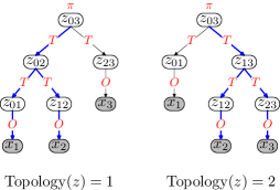
Figure 3: An example of a backbone structure in blue corresponding to the compound parameter $OT\operatorname*{diag}(T\pi)T^{\top}O^{\top}$, which appears in two different topologies, for two observation matrices, $\phi_{12}$ and $\phi_{23}$, respectively.

First, we will characterize the set of compound parameters graphically in terms of backbone structures. As an example, consider the PCFG-IE model and the observation matrix $\phi_{12}$ ($o=12$) corresponding to the marginal distribution over the first two words of the sentence. Given a topology $t$, consider starting at the root, descending to the lowest common ancestor of $x_{1}$ and $x_{2}$, and then following both paths down to $x_{1}$ and $x_{2}$, respectively. We refer to this traversal as the backbone structure with respect to topology $t$ and observation matrix $\phi_{12}$. See Figure 3 for an example of the backbone structure, outlined in blue.

Note that the compound parameter $\Psi_{12,t}(\theta)=\mathbb{E}_{\theta}[\phi_{12}(\mathbf{x})\mid\operatorname*{Topology}=t]$ can be written as a product over the parameter matrices, one for each edge of the backbone structure. For Figure 3, this would yield

$$\Psi_{12,1}(\theta)=OT\operatorname*{diag}(T\pi)T^{\top}O^{\top}.$$ (29)

For general trees, we would have

$$\Psi_{12,t}(\theta)=OT^{n_{1}}\operatorname*{diag}(T^{n_{3}}\pi)(T^{\top})^{n_{2}}O^{\top}.$$ (30)

for some positive integers $n_{1},n_{2},n_{3}$ corresponding to the number of edges (in $t$) from the common node to the preterminal node $z_{01}$, the preterminal node $z_{12}$, and the root $z_{0L}$, respectively.

Note that the compound parameter does not depend on the structure of $t$ outside the backbone—that part of the topology is effectively marginalized out—so the compound parameter $\Psi_{12,t}(\theta)$ will be identical for all topologies sharing that same backbone structure. Therefore, there are only a polynomial number of compound parameters despite an exponential number of topologies $t$.

We define a dynamic program that recursively computes $M_{op}$ for the PCFG-IE model under a fixed second-order observation matrix $\phi_{i_{0}j_{0}}$. Specifically, for each span ${[i:j]}$ define $H(i,j)$ to be the set of pairs $\left<t,n\right>$ where $t$ is a partial backbone structure $t$ and $n$ is the number of partial topologies over span ${[i:j]}$ which are consistent with $t$.

In the base case $H(i-1,i)$, if $i$ is either of the designated leaf positions defined by the observation matrix ($i_{0}$ or $j_{0}$), then we return the single-node backbone structure $\bullet$; otherwise, we return the null backbone structure ø:

$$H(i-1,i) =\begin{cases}\{\left<\text{\o},1\right>\}&\text{if $i=i_{0}$ or $i=j_{0}$}\\ \{\left<\bullet,1\right>\}&\text{otherwise}.\end{cases}$$ (31)

In the recursive case $H(i,j)$, we consider all split points $m$, partial backbones $t_{1}$ and $t_{2}$ from $H(i,m)$ and $H(m,j)$, respectively, and create a new tree with $t_{1}$ and/or $t_{2}$ as the subtrees if they are not null:

$$H(i,j) =\bigcup^{+}_{i<m<j}\bigcup^{+}_{\left<t_{1},n_{1}\right>\in H(i,m)}\bigcup^{+}_{\left<t_{2},n_{2}\right>\in H(m,j)}\left<\operatorname*{\text{\sc Combine}}(t_{1},t_{2}),n_{1}n_{2}\right>,$$ (32)

$$\operatorname*{\text{\sc Combine}}(t_{1},t_{2}) =\begin{cases}(T:t_{1},T:t_{2})&\text{if $t_{1}\neq\text{\o}$ and $t_{2}\neq\text{\o}$},\\ T:t_{1}&\text{if $t_{1}\neq\text{\o}$},\\ T:t_{2}&\text{if $t_{2}\neq\text{\o}$},\\ \text{\o}&\text{otherwise}.\end{cases}$$ (33)

Here, we use the notation $\bigcup^{+}$ to denote a multi-set union: $\{\left<t,n_{1}\right>\}\cup^{+}\{\left<t,n_{2}\right>\}=\{\left<t,n_{1}+n_{2}\right>\}$. In this notation, the backbone structure in Figure 3 would be represented as $T:(T:O:\bullet,T:O:\bullet)$, which can be easily converted to the compound parameter $OT\operatorname*{diag}(T\pi)T^{\top}O^{\top}$.

For third-order observation matrices (e.g., $\phi_{i_{0}j_{0}k_{0}\eta}$), we add an additional case to $H(i-1,i)$ to return $\left<\circ,1\right>$ if $i=k_{0}$; note that $k_{0}$ is represented by a special node $\circ$ because that observation is projected using $\eta$. The first case of $\operatorname*{\text{\sc Combine}}(t_{1},t_{2})$ undergoes one change: if $t_{2}$ is a chain ending in $\circ$, then we return $(T:t_{2},T:t_{1})$. The reason for this is best demonstrated by an example: consider topology 1 in Figure 3, and the two observation matrices $\phi_{132\eta}$ and $\phi_{231\eta}$. Without the reordering, we would have the backbone structure: $(T:(T:\bullet,T:\circ),T:\bullet)$ and $(T:(T:\circ,T:\bullet),T:\bullet)$. However, they have the same compound parameter $OT\operatorname*{diag}(T^{\top}O^{\top}\eta)T^{\top}\operatorname*{diag}(\pi)TO$. This is because the contribution of a subtree ending in $\circ$ is simply a diagonal matrix ($\operatorname*{diag}(T^{\top}O^{\top}\eta)$ in this case) which is applied on the hidden state regardless of whether it came from the left or right side.

References

- [1] A. Anandkumar, D. Hsu, and S. M. Kakade. A method of moments for mixture models and hidden Markov models. In COLT, 2012.
- [2] F. Pereira and Y. Shabes. Inside-outside reestimation from partially bracketed corpora. In ACL, 1992.
- [3] G. Carroll and E. Charniak. Two experiments on learning probabilistic dependency grammars from corpora. In Workshop Notes for Statistically-Based NLP Techniques, AAAI, pages 1–13, 1992.
- [4] M. A. Paskin. Grammatical bigrams. In NIPS, 2002.
- [5] D. Klein and C. D. Manning. Conditional structure versus conditional estimation in NLP models. In EMNLP, 2002.
- [6] D. Klein and C. D. Manning. Corpus-based induction of syntactic structure: Models of dependency and constituency. In ACL, 2004.
- [7] P. Liang and D. Klein. Analyzing the errors of unsupervised learning. In HLT/ACL, 2008.
- [8] J. T. Chang. Full reconstruction of Markov models on evolutionary trees: Identifiability and consistency. Mathematical Biosciences, 137:51–73, 1996.
- [9] A. Anandkumar, K. Chaudhuri, D. Hsu, S. M. Kakade, L. Song, and T. Zhang. Spectral methods for learning multivariate latent tree structure. In NIPS, 2011.
- [10] J. B. Kruskal. Three-way arrays: Rank and uniqueness of trilinear decompositions, with application to arithmetic complexity and statistics. Linear Algebra and Applications, 18:95–138, 1977.
- [11] E. S. Allman, C. Matias, and J. A. Rhodes. Identifiability of parameters in latent structure models with many observed variables. Annals of Statistics, 37:3099–3132, 2009.
- [12] E. S. Allman, S. Petrovi, J. A. Rhodes, and S. Sullivant. Identifiability of 2-tree mixtures for group-based models. Transactions on Computational Biology and Bioinformatics, 8:710–722, 2011.
- [13] J. A. Rhodes and S. Sullivant. Identifiability of large phylogenetic mixture models. Bulletin of Mathematical Biology, 74(1):212–231, 2012.
- [14] T. J. Rothenberg. Identification in parameteric models. Econometrica, 39:577–591, 1971.
- [15] L. A. Goodman. Exploratory latent structure analysis using both identifiabile and unidentifiable models. Biometrika, 61(2):215–231, 1974.
- [16] D. Bamber and J. P. H. van Santen. How many parameters can a model have and still be testable? Journal of Mathematical Psychology, 29:443–473, 1985.
- [17] D. Geiger, D. Heckerman, H. King, and C. Meek. Stratified exponential families: graphical models and model selection. Annals of Statistics, 29:505–529, 2001.
- [18] K. Lari and S. J. Young. The estimation of stochastic context-free grammars using the inside-outside algorithm. Computer Speech and Language, 4:35–56, 1990.
- [19] M. Johnson, T. Griffiths, and S. Goldwater. Bayesian inference for PCFGs via Markov chain Monte Carlo. In HLT/NAACL, 2007.
- [20] E. Mossel and S. Roch. Learning nonsingular phylogenies and hidden Markov models. Annals of Applied Probability, 16(2):583–614, 2006.
- [21] D. Hsu, S. M. Kakade, and T. Zhang. A spectral algorithm for learning hidden Markov models. In COLT, 2009.
- [22] S. M. Siddiqi, B. Boots, and G. J. Gordon. Reduced-rank hidden Markov models. In AISTATS, 2010.
- [23] A. Parikh, L. Song, and E. P. Xing. A spectral algorithm for latent tree graphical models. In ICML, 2011.
- [24] S. B. Cohen, K. Stratos, M. Collins, D. P. Foster, and L. Ungar. Spectral learning of latent-variable PCFGs. In ACL, 2012.
- [25] F. M. Luque, A. Quattoni, B. Balle, and X. Carreras. Spectral learning for non-deterministic dependency parsing. In EACL, 2012.
- [26] P. Dhillon, J. Rodue, M. Collins, D. P. Foster, and L. Ungar. Spectral dependency parsing with latent variables. In EMNLP-CoNLL, 2012.
- [27] J. Eisner. Three new probabilistic models for dependency parsing: An exploration. In COLING, 1996.
- [28] S. Sahni. Computationally related problems. SIAM Journal on Computing, 3:262–279, 1974.
- [29] J. Eisner. Bilexical grammars and their cubic-time parsing algorithms. In Advances in Probabilistic and Other Parsing Technologies, pages 29–62, 2000.