Effect of intracellular diffusion on current–voltage curves in potassium channels

Abstract

We study the effect of intracellular ion diffusion on ionic currents permeating through the cell membrane. Ion flux across the cell membrane is mediated by special proteins forming specific channels. The structure of potassium channels have been widely studied in recent years with remarkable results: very precise measurements of the true current across a single channel are now available. Nevertheless, a complete understanding of the behavior of the channel is still lacking, though molecular dynamics and kinetic models have provided partial insights. In this paper we demonstrate, by analyzing the KcsA current-­voltage currents via a suitable lattice model, that intracellular diffusion plays a crucial role in the permeation phenomenon. The interplay between the selectivity filter behavior and the ion diffusion in the intracellular side allows a full explanation of the current-­voltage curves.

I Introduction

Potassium currents across nerve membranes have been widely studied (see, e.g., HH ; NS ; Hille and the reviews GBOZ ; VanDongen02 ; Miller ; FH ; RCM ). Ionic channels selecting potassium currents are present in almost all types of cells in all organisms and they play many important and different functional roles.

Different types of measurements ADSEGHTM ; ZM provide a very detailed description of the behavior of potassium channels. In general, less is known on their structure Miller . KcsA, a potassium channel from Streptomyces lividans, is the first ion channel whose structure has been identified via X–ray crystallography doyle .

All ionic channels form selective pores in the cell membrane which open and close and, when in the open state, allow permeation of a selected ionic species (potassium in K⁺–channels). Their ability to open and close, i.e., gating, and their ability to allow the flux of a particular ionic species, i.e., selectivity, are not yet completely understood. A lot is known in the case of the KcsA channel and, with some care, can be extrapolated to the whole family of K⁺ channels.

In KcsA, see for instance the detailed description in Miller ; IOTS , gating is realized via four crossing transmembrane helices on the intracellular side. When in the open state, a spherical water–filled cavity of diameter about 10 Å  widens on the intracellular side of the channel up to the membrane plane. There a 10–15 Å  long and 3 Å  large channel containing the selectivity filter connects the cavity to the extracellular side.

When the channel flips to the open state a solution with the cytoplasm concentration reaches the entrance of the channel. Part of the ions permeates through the channel leaving an ion depleted region close to the pore. The typical time needed to restore the intracellular concentrations close to the pore will depend strongly on the diffusion process of ions inside the cell. We can then imagine that the current flowing through the channel will depend both on the diffusion of ions in the cytoplasm and on the behavior of the selectivity filter.

The problem of computing the permeation current in the open state, namely, the so called true current, has been approached theoretically by a large variety of methods. Molecular dynamics studies Aqvist ; BR give a very detailed description, but they usually do not provide macroscopic currents estimates due to the too small involved time scale. Kinetic models Miller02 ; Nelson ; MP ; Nelson02 ; Nelson03 ; MP ; VanDongen01 give very useful information, since electro–physiological experiments are performed over time scales much longer than the atomic one, with the drawback of the extreme simplification on the structure of the channel.

In the recent literature it has been examined the possibility to validate these kinetic models by comparing the predicted behaviors with those observed experimentally. In particular the models have been tested against their ability to predict the current–voltage behavior. In this respect very accurate experimental results have been published for different potassium channels, see MHM , SH , and HmK for the KcsA, MaxiK, and the Shaker channels, respectively.

Models such as those quoted above describe to some extent the dynamics of ion permeation through the selectivity filter, the concentration of the ion in the cell is introduced in the model as a constant parameter. In other words in those studies the diffusion of the ions inside the cell is not taken into account. Our opinion is that diffusion, as explained above, must take an important part in the permeation phenomenon. In ABCM01 , inspired by VanDongen01 , we introduced a model where the channel is lumped to a two state stochastic point system and the interaction between the dynamics of the ions inside the cell (diffusion) and that of the selectivity filter itself is taken into account. The channel is then thought of as part of the cell more than as an isolated structure. In that paper both an analytical and Monte Carlo study showed the possibility to achieve gating via selection.

In this paper we examine the possibility to predict the behavior of the current–voltage curves (graph of the permeation current vs. the external potential difference applied to the membrane) on the basis of a similar model. A modification is needed to take into account the effect of an external voltage difference through the cell membrane. The model is thus defined to mimic the three effects that seem to be the most relevant in the process: (i) diffusion of the ions inside the cell; (ii) dynamics of the selectivity filter; (iii) dynamics of the ions inside the selectivity filter. We compare the current–voltage behavior predicted by our model with experimental results from MHM ; SH ; HmK and find a very good agreement both for the dependence of the current on the ion concentration and on the external voltage.

Ion diffusion (item (i)) inside the cell is modeled as a symmetric random walk on a finite line. We use a one dimensional system in order to compute all the interesting quantities explicitly (ABCM01, , Appendix B). As we shall comment later the dimensionality of the system affects only our estimate of the diffusion coefficients of ions inside the cytoplasm. Corrections will be introduced to compute the three–dimensional value of the diffusion coefficient.

We remark that point (i) is the real distinguishing feature of our model. As we shall discuss later, the introduction of ion diffusion in the intracellular region and hence of the depletion phenomenon, will allow a full description of the permeation current behavior with respect to both external voltage and ion intracellular concentration.

One of the two boundary points of the finite line where ions diffuse is reflecting, whereas the other mimics the selectivity filter. The dynamics of the pore (item (ii)) is assumed to be stochastic. The pore jumps randomly between two states, the low and the high–affinity one. The dynamics of the pore is independent from that of the ions inside the cell. The chances that an ion has to enter the pore depend both on the ion species and on the pore state; in this way selection is implemented in the model.

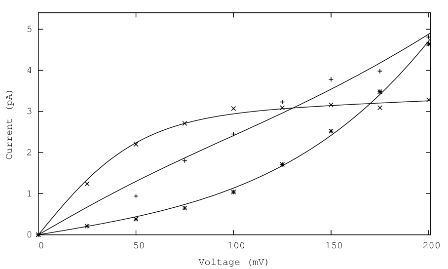
Figure 5: Comparison between experimental current–voltage curves MHM (symbols) and theoretical prediction (solid lines). The symbols $*$, $+$, and $\times$ refer respectively to Rb⁺, NH${}_{4}^{+}$, and Tl⁺ at concentration $100$ mM.

This description is quite faithful to the real behavior of the selectivity filter. Indeed, two possible states are possible for the filter RMFMPEAFGMG , the low and the high–affinity one. When the filter is in the low–affinity state permeation is favored, but no ionic species is preferred. Thus, in order to realize selectivity in an efficient way, the filter has to jump between these two states. To our knowledge the time fraction spent by the filter in the low affinity–state is not known experimentally; the value predicted by analyzing the current–voltage curves via our model depends on the ionic concentration in cytosol and is of order $10^{-3}$. This result seems to be coherent with the qualitative description given in (VanDongen01, , Figure 5).

The dynamics of the ions inside the filter (item (iii)) is not modeled in detail, we just assume that a particle inside the pore can either exit the system or reenter the cell with a fixed probability. This ejection probability is chosen as a function of the voltage difference across the cell membrane. Our modeling of the dynamics inside the filter is, thus, reduced to the choice of this function. It is worth noting that the model is able to reproduce accurately the experimental results with different choices of this function, that is to say with different descriptions of the dynamics of the ions inside the filter. More precisely we shall see that it is possible to explain the experimental results via different models for the dynamics of the ions inside the filter; when a different functional behavior for the ejection probability in terms of the external voltage is chosen, a different value of the typical time spent by the filter in the low–affinity state is found. In other words different models of the dynamics of the ions inside the filter are allowed provided the low–affinity state probability is changed suitably.

Indeed, we shall find very good results either by choosing the ejection probability function according to very well known and studied theories Nelson02 or by assuming that the ejection probability for a potassium ion trapped inside the filter is a power law function of the applied (suitably renormalized) voltage difference. In both cases our model will predict curves fitting cleanly the experimental result for the “true” ion current with reasonable values of the intracellular diffusion coefficient; but different values of the low–affinity state probability will be predicted. A more precise knowledge of this probability would enable us to discriminate among different mechanisms.

Moreover, we remark that our model will be also able to explain the behavior of ionic species different from potassium by choosing properly the physical parameters appearing in the ejection probability function of the external voltage difference.

We finally note that some care has to be used when the theoretical results are compared with experiments. In the biological literature, see for instance ADSEGHTM , two different types of current are reported, the apparent and the true one. This is connected with the peculiar behavior of ionic channels: two different states are observed, closed and open channel. In the first state a zero current is observed, in the second one the outgoing current fluctuates randomly on a very short time–scale and a not zero average current, called true current, is measured. The true current can be accessed experimentally only if the time resolution of the instruments is good enough to distinguish neatly between the open and the closed time intervals. When this is not the case a different current, called apparent current, is measured. This current is smaller than the true one since the instruments average the current also on time intervals in which the channel is closed.

The model we propose here is intended to mimic the behavior of the ionic channel in the open state. The average outgoing flux that will be computed has then to be thought as a prediction for the true current.

In Section II we introduce the lattice model. Section III is devoted to the analysis of the experimental data. Our results will be discussed in Section IV, where, in particular, we shall comment on the physical meaning of the fitting parameters introduced previously. Our conclusions are briefly summarized in Section V.

II The model

The intracellular region is modeled via a finite one–dimensional lattice $\Lambda\subset{\mathbb{Z}}$ with $L$ sites. Two sites of ${\mathbb{Z}}$ are said to be nearest–neighbors if and only if their mutual Euclidean distance is equal to one. The boundary $\partial\Lambda$ of $\Lambda$ is the collection of the two sites of ${\mathbb{Z}}$ not belonging to $\Lambda$ and neighboring one of the site of $\Lambda$. One of the two points of the boundary of $\Lambda$ is called pore, and denoted by $P$.

One ionic species performs an independent symmetric random walk on the lattice with reflectivity conditions on the site of $\partial\Lambda$ different from the pore. The particles on the site neighboring the pore behave in a special way that will be described below; due to the peculiarity of such a rule the walkers will turn out to be not independent. The number of walkers is denoted by $N$.

The fact that the walkers are independent on $\Lambda$ means that the position of a particle does not affect the motion of the others, in particular no constraint to the number of particles on each site is prescribed. The fact that the random walks are symmetric means that each jump between two neighboring sites of $\Lambda$ is performed with probability $1/2$. Since we assumed that the boundary is reflecting, particles in the site neighboring $\partial\Lambda\setminus\{P\}$ can stay in the same site with probability $1/2$.

Two states are allowed for the pore: high–affinity and low–affinity. The pore switches between the two states randomly; the probability that the pore is in the low–affinity state is denoted by $p\in[0,1]$. Moreover the pore can be either free or occupied by an ion. The behavior of the particles on the site $Q$ neighboring the pore depends on the state of the pore itself as it is precisely stated in figure 1. The idea is the following. If the pore is occupied by a particle, no other ion can enter it. If the pore is (free) in the low–affinity state, particles can enter it; when they enter the pore they immediately dissociate so that, with probability $v\in[0,1]$ they exit the system while they reenter $\Lambda$ with probability $1-v$. If the pore is free and in the high–affinity state, one particle can enter it, but, once entered, it remains there until the pore state changes to the low–affinity one. When this happens the ion dissociates with the same rule described above. As noted above, due to the pore rule, the walkers are not independent.

Whenever an ion exits the system another particle is put at random with uniform probability $1/L$ on one of the $L$ sites in $\Lambda$ so that the number of ions is kept constant.

The model described above is implemented with the Markov Chain described in detail in the appendix A. An iteration or sweep of the chain is the collection of the steps that are performed at each time $n$.

As we have explained in the Introduction, the aim of this paper is that of computing the outgoing ionic current. This quantity is related to the number of particles that exit the system. We let $M(n)$ be the number of particles which exited the system in the time interval $[0,n]$. Moreover, we let the flux at time $n$ be $M(n)/n$. Since we defined the stochastic process in such a way that the number of ions keeps constant in the volume $\Lambda$, $M(n)/n$ approaches a constant value $f$ for $n\to\infty$. This quantity, that we shall call the outgoing flux, is expected to be proportional to the “real” current measured experimentally.

The existence of this limiting flux can be deduced by remarking that the chain is irreducible and that the space state is finite. So we have that there exists a stationary measure for the process and that, in the limit $n\to\infty$, the time dependent quantities tend to the corresponding quantities averaged against the stationary measure.

By exploiting one–dimensionality, the model can be solved analytically and the outgoing flux can be computed explicitly. In our model the pore is modeled in a very simple fashion, indeed it is just a two state Bernoulli process; the main difficulty is, obviously, the interaction between the random walk inside the volume $\Lambda$ and the pore itself. We consider the stationary state reached by a walker and denote by $q$ the probability for the ion to occupy the site $Q$ of $\Lambda$ neighboring the pore.

Particles that enter the pore in the low–affinity state can exit the system with probability $v$. With the same probability a particle trapped in the pore in the high–affinity state can exit $\Lambda$ when the pore switches to the low–affinity state. We can write the outgoing flux as

$$f=\frac{1}{2}Nqpv+prv$$ (1)

where we have denoted by $r$ the probability that in the stationary state the pore is occupied by a particle when it switches from the high to the low–affinity state.

This one dimensional model can be solved following the same idea used in ABCM01 . We find

$$r=\frac{N+B+C-\sqrt{(N+B+C)^{2}-4NC}}{2C}$$ (2)

and

$$q=\frac{2p}{(1-p)(1-r)}\frac{r}{N}$$ (3)

where we have set

$$A=\frac{2L^{2}-3L+1}{3},\;\;B=\frac{2p}{1-p}\Big{(}L+\frac{v}{2}Ap\Big{)}$$

and

$$C=1+pAv$$

III Comparison with experimental results

In MHM it has been demonstrated that the KcsA, a bacterial ion channel of $K_{\textrm{ir}}$ topology and very well known structure (see, for instance, Miller and references therein), is a potassium channel. In that paper very precise measurements of potassium (and some other ion species) currents are reported. In this section we try to explain their results via our model.

Since the structure of the KcsA channel is well know, in this section will be mainly concerned with the experimental measures in MHM . At the end a brief analysis of the results in SH and HmK , concerning respectively the MaxiK and the Shaker channel, will be given. Note that the Shaker is a voltage–activated channel of $K_{\textrm{v}}$ topology.

III.1 Potassium current–voltage curves

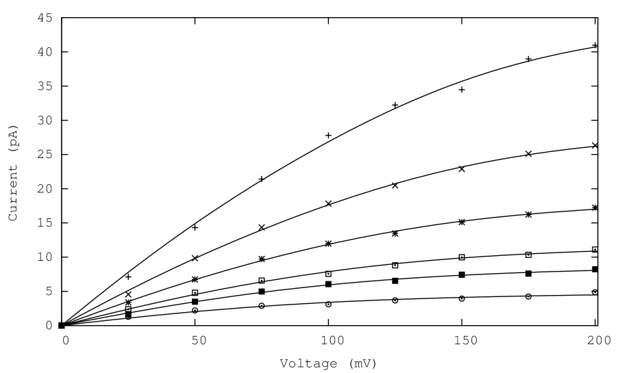
Figure 2: Comparison between experimental KcsA potassium current–voltage curves in MHM (symbols) and theoretical prediction (solid lines). The symbols $\bigcirc$, $\blacksquare$, $\square$, $*$, $\times$, and $+$ refer respectively to the potassium concentrations $20,50,100,200,400,800$ mM.

In (MHM, , Figure 2B) the potassium current–voltage curves at different concentrations $20,50,100,200,400,800$ mM are shown. We text the reliability of our lattice model by exhibiting neat fitting of those experimental data.

	KcsA						Shaker					MaxiK
$N$	$800$	$400$	$200$	$100$	$50$	$20$	$605$	$325$	$206$	$73$	$43$	$400$	$150$	$50$
$S_{I}$ ($10^{6}$ pA)	$3.83$	$4.91$	$6.33$	$8.07$	$12.0$	$16.7$	$1.00$	$1.03$	$1.31$	$2.09$	$3.03$	$7.56$	$7.03$	$8.88$
$p$ ($10^{-3}$)	$3.93$	$2.07$	$1.12$	$0.61$	$0.32$	$0.14$	$5.69$	$3.91$	$2.48$	$1.27$	$0.46$	$0.30$	$0.16$	$0.08$
$s$ ($10^{-14}$ sec)	$4.17$	$3.25$	$2.53$	$1.98$	$1.34$	$0.96$	$16.0$	$15.5$	$12.2$	$7.66$	$5.28$	$2.12$	$2.77$	$1.80$
$D$ ($10^{-2}$ cm2/sec)	$3.62$	$4.64$	$5.98$	$7.62$	$11.3$	$15.8$	$0.88$	$0.91$	$1.15$	$1.83$	$2.65$	$7.11$	$6.60$	$8.34$

Table 1: The parameters $S_{I}$ and $p$ have been measured by fitting the experimental data in MHM , HmK (data extracted from figure 1B therein), and SH via (4) and (5). By fitting the highest concentration set of data we also found $S_{V}=1.2\times 10^{-3}$, $\delta=0.19$, $l=5.5$ nm, and $L=1.00\times 10^{4}$ for the KcsA, $S_{V}=5.45\times 10^{-3}$, $\delta=0.16$, $l=5.3$ nm, and $L=1.12\times 10^{4}$ for the Shaker and $S_{V}=8.91\times 10^{-3}$, $\delta=0.16$, $l=5.5$ nm, and $L=1.00\times 10^{4}$ for the MaxiK. The parameters $s$ and $D$ have been computed via (8) and (9).

Let $I$ be the measured current, $V$ the voltage applied across the cellular membrane and write

$$I=S_{I}f$$ (4)

where $f$ is given in (1) with

$$v=S_{V}\frac{e^{\alpha\delta V}-e^{-\alpha\delta V}e^{-\alpha(1-2\delta)V}}{1+e^{-\alpha(1-2\delta)V}}$$ (5)

where $S_{I},S_{V},\delta$ are positive parameters and $\alpha$ is the constant $\alpha=e_{0}/K_{b}T=0.039$ mV^-1, with $e_{0}=1.6\times 10^{-7}$ pC the charge of the potassium ion, $K_{\textrm{b}}$ the Boltzmann constant, and $T=298.15$ ${}^{\textrm{o}}$K the temperature.

As we discussed in the Introduction, the choice of the probability $v$ as a function of the voltage $V$ is the only ingredient of the model related to the dynamics of the ions inside the filter. The choice (5) is inspired by the model in Nelson ; Nelson02 ; Nelson03 and dates back to the knock–on model in HK02 . We remark that, as it will be made clear in Section III.4, the ability of our model to describe the experimental results does not depend strictly on this choice. See also the comments there in this connection.

We fit the experimental data for concentration $800$ mM by using the above formula with $N=800$. In this way we fix the parameters

$$S_{I},\;S_{V},\;\delta,\;L,\textrm{ and }p_{800}$$

where $p_{800}$ is the low–affinity probability for concentration $800$ mM.

We complete the analysis of the data set according to the following scheme. The values of $S_{I}$ and $p$ for the six experimental series are supposed to change, that is to say we assume that the probability that the filter is in the low–affinity state and the constant $S_{I}$ (we will see in Section IV that this constant is related to the diffusion coefficient in the intracellular region) depend on the ionic concentration. The five other experimental series, that is to say those measured at concentrations $400,200,100,50$, and $20$ mM, are then fitted by the same equation by keeping fixed $S_{V}$, $\delta$, $\alpha$, and $L$ and by using $p$ and $S_{I}$ as the sole fitting parameters. Results are plotted in figure 2; the fitted parameters are reported in table 1. The physical meaning of the fitting parameters will be discussed in Section IV.

This fitting scheme is based on a simple remark: we assume that the channel behavior, that in our description is modeled by the function (5), does not depend on the ion concentration. On the other hand we cannot exclude that the ionic diffusion coefficient in the intracellular region HS and the typical time spent by the pore in the low–affinity state depend on the concentration of the ionic species in the cell.

The soundness of the values that we found for the fitting parameters will be discussed in Section IV. We now mention only two facts: to our knowledge there exists no experimental measure of the time fraction spent by the filter in the low–affinity state. So that we cannot say anything about the validity of our estimate for $p$; we can just remark the qualitative agreement with (VanDongen01, , Figure 5). The estimated diffusion coefficient is several orders of magnitude larger than the real (experimental) value HS ; HK . This expected problem is due to the one–dimensional character of the model. In Section IV we shall compute the associated three–dimensional estimates that will result to be in very good agreement with the experimental values.

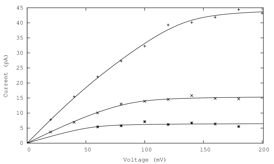
Figure 3: Comparison between experimental MaxiK potassium current–voltage curves in SH (symbols) and theoretical prediction (solid lines). The symbols $*$, $\times$, and $+$ refer respectively to the potassium concentrations $50,150,400$ mM.

Finally we note that with our fitting scheme we also are able to reproduce with good accuracy the data in SH , and HmK referring, respectively, to the MaxiK and Shaker channel in HmK (see figure 3 and table 1). Data in figure 3 have been reproduced with the authors’ permission. The data related to the Shaker channel have been extracted from figure 1B in HmK .

III.2 Potassium conductance curves

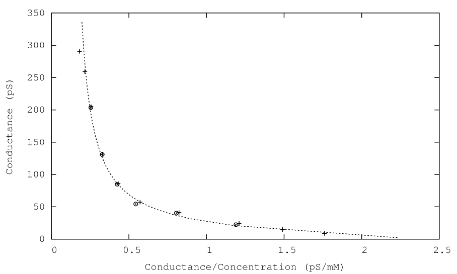
Figure 4: The Eadie-Hofstee plot for the potassium permeation current at external voltage $200$ mV. The symbols $+$ and $\bigcirc$ refere, respectively, to the experimental data and to the theoretically computed values. The dotted line is an eye guide.

In MHM the permeation behavior of the pore has been investigated also by means of the conductance $g=I/V$. We compared the permeation data in MHM at fixed voltage $V=200$ mV and concentration varying from $5$ mM to $1600$ mM, with the results of our fit of potassium current–voltage curves (see Section III.1), as shown in figure 4 by an Eadie–Hofstee plot. In the picture the symbols $+$ and $\bigcirc$ refer, respectively, to the experimental data and to the theoretically computed values, whereas the dotted line is an eye guide.

The matching is good in the whole region where full experimental data sets are known. This graph shows neatly the ability to our model to capture also the dependence of the permeation current on the ion intracellular concentration.

Even if we do not have any physical argument to support this choice, it is worth noting that the dotted line in the picture, which is just an eye guide, has been indeed obtained by assuming a (slightly sub–linear) power low dependence of the low–affinity state probability $p$ on the ion concentration and an Hill type behavior for the diffusion coefficient.

	$NH4^{+}$	$Tl^{+}$	$Rb^{+}$
$\delta$	$0.17$	$0.017$	$0.33$
$S_{V}$	$3.2\times 10^{-4}$	$6.8\times 10^{-4}$	$9.4\times 10^{-5}$

Table 2: Parameters measured by fitting the experimental data for ions different from potassium in KcsA via (4) and (5). Recall also that $N=100$, $S_{I}=8.07\times 10^{6}$, $p=6.1\times 10^{-4}$, $s=1.98\times 10^{-14}$ sec, $D=7.62\times 10^{-2}$ cm²/sec and $L=10^{4}$.

III.3 Other species current–voltage curves

We test our model against the experimental current–voltage curves MHM for ions different from potassium. More precisely we consider the curves for NH${}_{4}^{+}$, Tl⁺, and Rb⁺ at ionic concentration 100 mM.

To fit these curves we fix the values of $S_{I}$, $L$, and $p$ to the ones found previously for potassium at concentration 100 mM, and we use $\delta$ and $S_{V}$ as fitting parameters. That is to say that we assume that the ionic diffusion in the intracellular region and the probability of finding the filter in the low–affinity state are independent on the ionic species, but depend only on the ionic concentration. This is suggested by the measured values of the diffusion coefficient, see for instance (CZSO, , Table 2) for Tl⁺ and (Cussler, , Table 1.1-1) for the other ions.

With this assumption we are implicitly saying that the reduced, with respect to potassium, permeation rates typical of the other selected ion species is due to the behavior of such ions inside the selectivity filter. Results are plotted in figure 5; the fitted parameters are reported in table 2.

Deeper investigation on this point should be corroborated by additional data. As in the potassium case, data sets corresponding to different values of the intracellular concentrations are needed.

III.4 Modeling the channel

In the discussion above the choice of the relation between the ejection probability and the voltage across the membrane, see equation (5), has been inspired by the physical argument proposed in the kinetic model for single–file ion channels in Nelson ; Nelson02 ; Nelson03 . The function in (5) has the same form of the channel permeation rate used in that model, that is to say we are assuming that the inner part of the channel behaves like a single file ion channel. One of the key novelties in our work is the coupling between this mechanism and the diffusion of the ions in the intracellular region.

It is worth noting that the analysis conducted in Subsections III.1, III.2, and III.3 can be repeated using a simple power law (having no particular physical meaning) for the ejection probability as a function of the external voltage. In other words we can assume

$$v=\Big{(}\frac{V}{C_{V}}\Big{)}^{\gamma}$$ (6)

for modeling the relation between the ejection probability and the voltage across the membrane.

In this case we get similarly good results, that is to say we are able to reproduce the experimental data with good precision. We do not show the graphs, which are similar to those in figure 2, but report the whole set of fitted parameters in table 3.

This remark suggests that, in the framework of our model, no particular modeling of the dynamics of ions inside the channel is needed in order to get the correct behavior of the current–voltage curves. But it is important to remark that different filter models produce different values for the time fraction spent by the selectivity filter in the low–affinity state. Indeed, see tables 1 and 3, by using the models (5) and (6) for the dynamics inside the filter, similar values for the diffusion coefficient are found, whereas the predictions for the time fraction $p$ spent by the selectivity filter in the low–affinity state differ by an order of magnitude. This suggests that the current–voltage curves could be a useful instrument to predict the time fraction spent by the selectivity filter in the low–affinity state once the dynamics of the ions in the filter is known or vice–versa.

	KcsA
$N$	$800$	$400$	$200$	$100$	$50$	$20$
$S_{I}$ ($10^{6}$ pA)	$4.47$	$6.03$	$7.71$	$9.73$	$14.5$	$19.6$
$p$ ($10^{-2}$)	$3.02$	$1.77$	$1.14$	$0.82$	$0.45$	$0.39$
$s$ ($10^{-14}$ sec)	$3.38$	$2.65$	$2.07$	$1.64$	$1.11$	$0.82$
$D$ ($10^{-2}$ cm2/sec)	$4.47$	$5.70$	$7.29$	$9.20$	$13.7$	$18.5$

Table 3: The parameters $S_{I}$ and $p$ have been measured by fitting the experimental data in MHM via (4) and (6). By fitting the highest concentration set of data we also found $C_{V}=6.31\times 10^{4}$, $\gamma=1.19$, $l=5.5$ nm and $L=1.00\times 10^{4}$. The parameters $s$ and $D$ have been computed via (8) and (9).

IV Discussion

In the above section we have seen that the model proposed in this paper is able to explain in great detail the experimental data for the current–voltage curves in the KcsA ionic channel. We have shown that the theoretical predictions fit nicely the measured curves provided the parameters defining the model are suitably chosen. It is notable that our model explains the dependence of the permeation current both on the external voltage (figures 2, 3, and 5) and on the ion concentration in the intracellular region (figure 4).

In Nelson02 the same experimental data MHM have been analyzed via a kinetic model formerly introduced by the same author. In that model the selectivity filter is treated as an isolated structure and the intracellular ion concentration is an input constant of the model. Two different regimes for the filter had to be assumed corresponding, respectively, to high (400 mM and 800 mM) and low (20 mM, 50 mM, and 100 mM) potassium concentrations. Two different sets of the parameters carachterizing the filter behavior (the analogue of $S_{V}$ and $\delta$) were found.

In other words the model in Nelson02 predicts that the behavior of the selectivity filter depends on the intracellular ion concentration. In our model the selectivity filter is coupled with the diffusion of ions in the intracellular region; this is indeed the key novelty and the distinguishing feature of our approach. This allows to explain the experimental data referring to all the concentrations with the same set of parameters, $S_{V}$ and $\delta$, for the filter behavior.

To compare the way in which data are explained by the model in Nelson02 and by our model, we first note that the electrical dissociation distance $\delta$ (see (Nelson, , Fig. 1)) that we find is very close to that fitted there. Moreover, we note that in Nelson02 in the lower intracellular concentration regime, the fitted parameters are such that an higher effective concentration ($c^{*}$ in their notation) is seen. In our model particle diffusion accounts for this effect.

We now discuss the reasonableness of the values we found for these fitting parameters for the potassium current data for the KcsA ionic channel (see Section III.1).

As a first step we have to give a continuum interpretation of the lattice modeling the cytosol. In other words we have to associate with the unit length of the lattice model a physically reasonable quantity. We imagine to associate with each lattice site a small cubic volume whose side length is denoted by $\ell$. Recall that the experimental concentration $c$ is expressed in millimolar, that is as number of moles per cubic meter (i.e., number of millimoles per liter). Recall, also, that $N$ is the number of particles in the lattice model and that $L$ is the number of sites in $\Lambda$. We then have the following identification

$$c=\frac{N}{N_{\textrm{A}}}\frac{1}{\ell^{3}L}$$

where $N_{\textrm{A}}=6.022\times 10^{23}$ is the Avogadro number and $\ell$ has to be expressed in meter.

Since in our fitting procedure we have chosen $N$ such that $c/N=1$ mM, we have that

$$\ell=\frac{1}{(N_{\textrm{A}}L)^{1/3}}=5.50\times 10^{-10}~{}\textrm{m}=0.55~{}\textrm{nm}$$ (7)

where we have used that $L$ has been fitted to $10^{4}$, see the caption of table 1. The above argument provides us with a way to associate a length unit measure with our lattice model. The result we found for $\ell$ is physically reasonable, indeed we can assume that each cubic volume associated with a site of the lattice can accommodate few (say one or two) ions, so that its side length has to be of the order of magnitude of the ionic diameter. This value we found for $\ell$ is then reasonable, since potassium ion, atomic, and van der Waals radius are respectively given by $0.13,0.23$, and $0.27$ nm.

As a second step we have to give a continuum interpretation of the discrete unit of time of the Markov Chain. In other words we have to associate with the unit of time a physically reasonable quantity $s$. We consider the evolution of our model up to the time $n$ and note that the true current measured in the experiments can be identified as

$$I=\frac{e_{0}\times\textrm{(number of particles which exited }\Lambda\textrm{)}}{s\times\textrm{(number of iterations)}}=\frac{e_{0}}{s}\,f$$

where $e_{0}=1.6\times 10^{-7}$ pC is the charge of a potassium ion and $f$ is the theoretical model outgoing flux. We then identify $e_{0}/s$ with the parameter $S_{I}$ introduced in equation (4); that is to say we write

$$s=\frac{e_{0}}{S_{I}}$$ (8)

and we can use the estimated $S_{I}$ listed in the first row of table 1 to compute the values of $s$ listed in the same table.

We have no direct clue to establish if these values for $s$ are reasonable or not. But starting from this values we can estimate the diffusion coefficient of potassium ions in the cytosol. Indeed, see Appendix B, the intracellular ion diffusion coefficient is related to the other parameters by the equation (10), which yields

$$D=\frac{\ell^{2}}{2s}$$ (9)

By using this equation we compute the diffusion coefficient for the potassium. Results have been reported in the last row of table 1.

The order of magnitude we found for the diffusion coefficient of potassium ions is $10^{-2}$ cm${}^{2}/$sec. This result is several (say three) order of magnitude larger than the real (experimental) value HK . This problem was indeed quite expected, since we modeled the diffusion of ions in cytosol with a one–dimensional lattice. As we have already remarked, the one–dimensional choice is motivated by the possibility to write explicitly the solution of the probabilistic model. Explicit formulas are quite necessary to perform the extended analysis discussed in Section III. As a future work we are now planning a Monte Carlo assisted analysis for the three–dimensional version of our model.

In any case we prove, now, that the estimates we found in this one–dimensional case for the diffusion coefficient are quite reasonable. Consider a simple symmetric random walk with unitary time on a three-dimensional cubic lattice with $L$ sites and spacing $m$. We consider the side length $L^{1/3}$ in order to ensure that the “real” volume associated with the three dimensional model is equal to that associated with the one dimensional one. By a classical argument similar to the one developed in the Appendix B it is proven that the squared mean distance walked up to time $t$ is $6D_{3}t$ where $D_{3}$ is the diffusion coefficient. This implies that the typical time needed by the walker, started at random in the lattice, to reach a particular point of the boundary (say the pore) is of order

$$\frac{(mL^{1/3})^{2}}{64}\times\frac{1}{6D_{3}}\times 6(L^{1/3})^{2}$$

Indeed, the first term is the square of the average distance of a point inside a cube of side length $mL^{1/3}$ from the boundary of the cube itself and the third one is the number of times the walker has to visit the boundary before touching the pore (number of points on the lateral surface of the cube). Note that the product between the first and the second term is an estimate for the time needed to touch the boundary of the cube for a walker started at random in the cube itself.

In our former analysis, in computing fluxes, we indeed evaluated this time in the framework of our one–dimensional model. By repeating the same argument we can say that this time was estimated as

$$\frac{1}{16}(mL)^{2}\times\frac{1}{2D_{1}}\times 2$$

By equating the two expressions found above we find

$$D_{3}=\frac{1}{4}D_{1}L^{-2/3}\approx 0.00054\times D_{1}$$

where we used $L=10^{4}$ (see the caption of table 1). By the equation above it follows that to the diffusion constant estimated via the one–dimensional model ranging in $3.62$ – $15.8\times 10^{-2}$ cm²/sec (see table 1) it corresponds a “true” diffusion coefficient ranging in $1.95$ – $8.53\times 10^{-5}$ cm²/sec, which is very close to the experimental value for the potassium diffusion coefficient HK .

V Conclusions

In this paper we have studied the effect of intracellular ion diffusion on ionic currents permeating through the cell membrane ionic channels. Ion channels share the following common properties: the ion flux is rapid, the channel is selective, and its functions are regulated by a gating mechanism. Although a formidable effort, with absolutely remarkable results, has been performed recently, a complete understanding of ionic channel behavior is still lacking.

Thanks to the patch clamp technique very precise measurements of the true current across a single channels are available. In this paper we have proposed a model which is able to provide a full explanation of the KscA current–voltage experimental curves MHM by taking into account the following three effects: ion diffusion in the intracellular region, dynamics of the filter, and dynamics of the ions inside the filter.

In particular our model points out the role played by intracellular diffusion on ion permeation in compensating the ion depletion in the region close to the pore. The model is able to explain the dependence of the experimetal data referring to the true ionic currents both on the external voltage and on the intracellular potassium concentration.

Is is also notable that all the fitting parameters have a clear qualitative and quantitative physical interpretation. Moreover, we noted that the estimate we got for the typical time spent by the filter in the low–affinity state is strictly related to the dynamics of ions inside the filter. This suggests that our approach, corroborated by new experimental data, should be able to shed some light also on the dynamics of the ions inside the filter.

Appendix A Detailed definition of the model

We consider an integer time variable $n$. We set $n=0$ and choose at random with uniform probability $1/L$ the position of the $N$ particles. We then repeat the following steps:

1. set $n$ equal $n+1$;

2. select at random the state of the pore: choose the low–affinity state with probability $p$ and the high–affinity one with probability $1-p$;

   1. if the pore is in the low–affinity state and it is occupied by a particle, the particle is released with the following rule: it jumps with probability $1-v$ to the site of $\Lambda$ neighboring the pore or, with probability $v$, it exits the system;

   2. if a particle exits the system, a particle of the same species is put at random with uniform probability $1/L$ on one of the $L$ sites in $\Lambda$;

3. the position of each particle on the lattice is updated following the rules defined in Section II;

   1. if a particle enters the pore and the pore is in the low–affinity state, the particle is immediately released by the pore with the following rule: it jumps with probability $1-v$ to the site of $\Lambda$ neighboring the pore or, with probability $v$, it exits the system;

   2. if a particle exits the system, a particle of the same species is put at random with uniform probability $1/L$ on one of the $L$ sites in $\Lambda$.

Appendix B Diffusion coefficient

Consider a one–dimensional walker on $\ell{\mathbb{Z}}$ and denote its position at time $t\in s{\mathbb{Z}}_{+}$ by

$$S_{t}\in\{\dots,-\ell,0,+\ell,\dots\}$$

The random variable $S_{t}$ is the sum of $t/s$ (note that $t/s$ is a positive integer) independent identically distributed random variables $Y_{i}\in\{-\ell,+\ell\}$ such that

$${\mathbb{P}}(Y_{i}=+\ell)={\mathbb{P}}(Y_{i}=-\ell)=\frac{1}{2}$$

A straightforward computation yields

$${\mathbb{E}}[Y_{i}]=0\textrm{ and }{\mathbb{E}}[(Y_{i}-{\mathbb{E}}[Y_{i}])^{2}]=\ell^{2}$$

for the average and the variance of the random variable $Y_{i}$ respectively. By independence we also get

$${\mathbb{E}}[S_{t/s}]=0\textrm{ and }{\mathbb{E}}[(S_{t/s}-{\mathbb{E}}[S_{t/s}])^{2}]=\frac{t}{s}\ell^{2}$$

By the Central Limit Theorem (see, for instance, (GS, , Theorem (4) in Section 5.10)) we have that for $t$ large the probability density of the random variable $S_{t/s}$ is very well approximated by the Gaussian

$$\frac{1}{\sqrt{2\pi\ell^{2}(t/s)}}\exp\{-x^{2}/[2\ell^{2}(t/s)]\}$$

for $x\in{\mathbb{R}}$. By comparing this result with the continuum description given by a one–dimensional diffusion equation $\dot{u}=Du^{\prime\prime}$ with diffusion coefficient $D$ we get the identification

$$2Ds=\ell^{2}$$ (10)

allowing to compare lattice and continuum results.

Figure 1: Rule for the site close to the pore. The black solid circle denotes the pore, the open circles denote sites of the lattice, the black arrows denotes jumps that are performed with probability $1/2$, the black lines denote jumps that cannot be performed (probability zero). On the left the behavior of an ion close to the pore in the high–affinity state is depicted: if the pore is free, the particle jumps with uniform probability $1/2$ to one of the $2$ nearest neighboring sites; if the pore is occupied, the particle jumps with uniform probability $1/2$ to the nearest neighboring site in the lattice (it cannot enter the pore) and with probability $1/2$ the particle does not leave the site. On the right the behavior of an ion close to the pore in the low–affinity state is depicted: the particle jumps with uniform probability $1/2$ to one of the $2$ nearest neighboring sites; If the pore is in the low–affinity state, the ions behave with the same rule as that for an ion faced to the free pore in the high–affinity state. It is worth remarking that the pore in the low–affinity state cannot be occupied.

- (1) A.L. Hodgkin and A.F. Huxley, J. Physiol. 116, 473 (1952).
- (2) E. Neher and B. Sakmann, Nature 260, 799 (1976).
- (3) B. Hille, “Ion Channels of Excitable Membranes,” Third Edition, Sinauer Associates Inc., Sunderland, MA, Usa, 2001.
- (4) S.A.N. Goldstein, D. Bockenhauer, I. O’Kelly, and N. Zilberberg, Nature Reviews Neuroscience 2, 175 (2001).
- (5) A.M.J. VanDongen, Comm. Theor. Biol. 2, 429 (1992).
- (6) C. Miller, Genome Biology 1 reviews0004 (2000).
- (7) D. Fedida and J.C. Hesketh, Prog. Bio. Mol. Biology 75, 165 (2001).
- (8) M. Recanatini, A. Cavalli, and M. Masetti, ChemMedChem 3, 523 (2008).
- (9) A. Abenavoli, M.L. Di Francesco, I. Schroeder, S. Epimoshko, S. Gazzarini, U.P. Hansen, G. Thiel, and A. Moroni, J. Gen. Physiol. 134, 219 (2009).
- (10) Y. Zhou and R. Mackinnon, J. Mol. Biol. 333, 965 (2003).
- (11) D.A. Doyle, C.J. Morais, R.A. Pfuetzner, A. kuo, J.M. Gulbis, S.L. Cohen, B.T. Chait, R. MacKinnon, Science 280, 69–77 (1998).
- (12) S. Imai, M. Osawa, K. Takeichi, I. Shimada, PNAS 107, 6216–6221 (2010).
- (13) J. Åqvist and V. Luzhkov, Nature 404, 881 (2000).
- (14) S. Bernèche, B. Roux, PNAS 100, 8644–8648 (2003).
- (15) C. Miller, J. Gen. Physiol. 113, 783 (1999).
- (16) P.H. Nelson, J. Chem. Phys. 117, 11396 (2002).
- (17) P.H. Nelson, Phys. Rev. E 68, 061908 (2003).
- (18) P.H. Nelson, J. Chem. Phys. 134, 165102 (2011).
- (19) S. Mafé and J. Pellicer, Phy. Rev. E 71, 022901 (2005).
- (20) A.M.J. VanDongen, PNAS 101, 3248 (2004).
- (21) M. LeMasurier, L. Heginbotham, and C. Miller J. Gen. Physiol. 118, 303–313 (2001).
- (22) I. Schroeder, U.P. Hansen, J. Gen. Physiol. 130(1), 83 (2007).
- (23) L. Heginbotham, R. MacKinnon, Biophysical Journal 65, 2089–2096 (1993).
- (24) D. Andreucci, D. Bellaveglia, E.N.M. Cirillo, S. Marconi, Physical Review E 84, 021920 (2011).
- (25) M.L. Renart, E. Montoya, A.M. Fernández, M.L. Molina, J.A. Poveda, J.A. Encinar, J.L. Ayala, A.V. Ferrer–Montiel, J. Gómez, A. Morales, and J.M. González Ros, Biochemistry 51, 3891–3900 (2012).
- (26) A.L. Hodgkin and R.D. Keynes, J. Physiol. 128, 61 (1955).
- (27) H.S. Harned and J.A. Shropshire, J. of the American Chemical Society 80, 5652–5653 (1958).
- (28) A.L. Hodgkin and R.D. Keynes, J. Physiol. 119, 513–528 (1953).
- (29) M. Ciszkowska, L. Zeng, E.O. Stejskal, and J.G. Osteryoung J. Phys. Chem. 99, 11764–11769 (1995).
- (30) E.L. Cussler, “Diffusion.” Second Edition, Cambridge University Press, Cambridge, UK, 1997.
- (31) G. Grimmet, D. Stirzaker, “Probability and Random Processes.” Oxford University Press Inc., New York, US, 2001.