Strangeness physics at MAMI: First results and perspectives

Abstract

During the last two years several experimental approaches to strange systems have been realized at the spectrometer facility of the Mainz Microtron MAMI. An instrument of central importance for the strangeness electro-production program is the magnetic spectrometer Kaos that was installed during 2003–8 and is now operated by the A1 collaboration in $(e,e^{\prime}K)$ reactions on the proton or light nuclei. Since 2008 kaon production at low four-momentum transfers off a liquid hydrogen target was studied. The measurements were sensitive to details of the phenomenological models describing the reaction. Two very prominent isobar models, Kaon-Maid and Saclay-Lyon A, differ in the number of contributing nucleon resonances and their longitudinal couplings at the kinematics measured at MAMI. In order to use Kaos as a zero-degree double-arm spectrometer a magnetic chicane comprising two compensating sector magnets was constructed and a new electron-arm focal-plane detector system was built.

I Introduction

The Mainz Mikrotron MAMI at the Institut für Kernphysik in Mainz is an accelerator to study the hadron structure with the electromagnetic probe. The machine has been upgraded to 1.5 GeV electron beam energy by a harmonic double-sided microtron Kaiser2008 . This fourth stage, called MAMI-C, was completed in 2007. With MAMI-C the threshold beam energy for associated strangeness production off protons was reached for the first time at MAMI.

The electromagnetic production of kaons off the nucleon provides an important tool for understanding the dynamics of hyperon-nucleon systems. Theoretically, the process is described often by effective Lagrangian models, commonly referred to as “isobar” approach. In the isobaric models the reaction amplitudes are constructed from lowest-order (so-called tree-level) Born terms with the addition of extended Born terms for intermediate particles, $N$, $K$, or $Y$ resonances, exchanged in the $s$-, $t$-, and $u$-channels. A complete description of the reaction process would require all possible channels that could couple to the initial and final state. Most of the model calculations for kaon electrophoto-production have been performed in the framework of tree-level isobar models Adelseck1990 ; Williams1992 ; Bennhold1999 , however, few coupled-channels calculations exist Feuster1999 . The drawback of the isobaric models is the large and unknown number of exchanged hadrons that can contribute in the intermediate state of the reaction. Depending on which set of resonances is included, very different conclusions about the strengths of the contributing diagrams for resonant baryon formation and kaon exchange may be reached. The Kaon-Maid and Saclay-Lyon models characterise our present understanding of kaon photoproduction reactions at photon energies below 1.5 GeV. The model SLA is a simplified version of the full Saclay-Lyon model in which a nucleon resonance with spin-5$/$2 appears in addition.

The electro-production of strangeness introduces two additional contributions, that are vanishing for the kinematic point at $Q^{2}=$ 0: the longitudinal coupling of the photons in the initial state, and the electromagnetic and hadronic form factors of the exchanged particles. Concerning the differential cross-section the model variations are strongest at small kaon centre-of-mass angle. To conclude, it is fair to say that new experimental data on strangeness production will challenge and improve our understanding of the strong interaction in the low energy regime of QCD.

II Elementary Kaon Electroproduction at MAMI

Tab. 1: Experimental setting of the kaon electro-production beam-time in 2009. The beam energy was 1.508 MeV, beam intensity 1–4 $\mu$A, beam raster size $\pm$ 1 mm, and the $\ell$H₂ target length 48 mm.

virt. photon + target				electron arm		kaon arm
$\langle Q^{2}\rangle$	$\langle W\rangle$	$\langle\epsilon\rangle$	$\langle\omega\rangle$	$\langle q^{lab}_{e^{\prime}}\rangle$	$\langle\theta^{lab}_{e^{\prime}}\rangle$	$\langle p^{lab}_{K}\rangle_{\Lambda}$	$\langle p^{lab}_{K}\rangle_{\Sigma}$	$\langle\theta^{lab}_{K}\rangle$
(GeV$\!/c$)2	GeV	(trans.)	GeV	GeV$\!/c$	deg	GeV$\!/c$	GeV$\!/c$	deg
0.036	1.750	0.395	1.182	0.318	15.5	0.642	0.466	$-$31.5

First experiments on the electro-production of kaons off a liquid hydrogen target were performed since 2008. Positive kaons were detected in the Kaos spectrometer in coincidence with the scattered electron into spectrometer B. The central spectrometer angle of the kaon arm was 31.50^∘ with a large angular acceptance in the dispersive plane of $\vartheta_{K}=$ 21–43^∘. The spectrometer setting for electron detection was fixed at the minimum in-plane angle of $\vartheta_{e^{\prime}}\approx$ 15^∘, thereby maximising the virtual photon flux. The invariant momentum transfer, $\langle Q^{2}\rangle=-\langle q^{2}\rangle$, was very low, the virtual photon energy, $\langle\omega\rangle$, was near the maximum of the kaon photoproduction cross-section at 1–1.2 GeV, which excites a total energy in the virtual-photon-nucleon center-of-mass system, $W^{2}=M_{targ}^{2}+2\omega M_{targ}-Q^{2}$, of 1.6–1.7 GeV. The kinematic conditions are summarised in Table 1. The cryogenic target in the spectrometer hall that was used for the kaon electro-production experiments consists of a 49.5 mm long target cell and is made of a 10 $\mu$m Havar walls. The geometry of the cell is optimized for enhancing the luminosity while keeping low the energy-losses.

III Kaon Identification

Kaon identification is based on specific energy-loss and time-of-flight, electron identification on a signal in a gas Cherenkov counter. Measured time-of-flight and specific energy-loss spectra are shown in Fig. 1 as a function of particle momentum. The time-of-flight was corrected for the path-length dispersion assuming the particle was a pion. The data sample is dominated by background particles (p and $\pi$) because of a kaon-to-background ratio of 1 : 200 and the event sample was enriched in kaon events by a cut in missing mass to show the position of the band of kaons in relation to the two bands from the dominant particle species. The flight time difference between protons and kaons is 10–15 ns, between pions and kaons 5–10 ns. The energy-loss separation between kaons and pions is small, whereas the separation between kaons and protons is of the order of 2–5 MeV$\!/$cm.

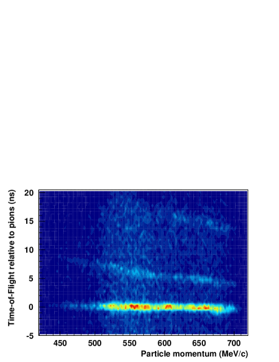
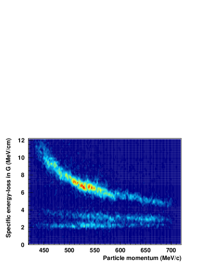
Fig. 1: Measured time-of-flight (left) and specific energy-loss (right) spectra in scintillator wall G as a function of particle momentum. The time-of-flight was corrected for the path-length dispersion assuming the particle was a pion. The event sample was enriched in kaon events by a cut in missing mass. Protons, kaons, and pions (curves from top to bottom) are separated.

After electron and kaon identification the measured momenta, in magnitude and direction with respect to the incoming beam, allow for a full reconstruction of the missing energy and missing momentum of the recoiling system. The missing mass $M_{X}$ is related to the four-momentum $q^{\mu}$ of the virtual photon and the four-momentum $p_{K}^{\mu}$ of the detected kaon according to $M^{2}_{X}=(q^{\mu}+P^{\mu}_{targ}-p^{\mu}_{K})^{2}$, where $P^{\mu}_{targ}=(M_{targ},\vec{0})$ is the target four-momentum. The missing energy and missing momentum can then be calculated using

$$E_{X} = E_{e}-E_{e^{\prime}}+M_{targ}-E_{K}=\omega+M_{targ}-E_{K},$$ (1)

$$\vec{P}_{X} = \vec{q}-\vec{p}_{K},$$ (2)

and the missing mass in terms of the kinematic variables $Q^{2}$, $\omega$, and $\vec{q}$ as well as of the reconstructed kaon energy, momentum, and scattering angle, can be written as

$$M_{X}=\sqrt{E^{2}_{X}-|\vec{P}_{X}|^{2}}=\sqrt{(\omega-E_{K}+M_{targ})^{2}+p_{K}^{2}-2p_{K}|\vec{q}|\cos{\theta_{K}}-Q^{2}}\,.$$ (3)

A preliminary missing mass spectrum is shown in Fig. 2 (left). The overlaid histograms show the missing mass distributions in two averaged $(e^{\prime},K)$ coincidence-time side-bands with the appropriate weights and additional kaon background. The large momentum acceptance of the Kaos spectrometer covers the free electro-produced hyperons $\Lambda$ and $\Sigma^{0}$. The well-known masses of the two hyperons can serve as an absolute mass calibration. Fig. 2 (right) shows the background-subtracted missing mass distribution compared to the Monte Carlo spectrum. The simulation includes radiative corrections, energy-loss in the target, and a model for the resolutions.

Fig. 2: Preliminary missing mass spectra in the p$(e,e^{\prime}K^{+})Y$ reaction. Left: Missing mass distribution with overlaid histograms showing random coincidences in two averaged $(e^{\prime},K)$ coincidence-time side-bands with the appropriate weights and additional kaon background. The $\Lambda$ and $\Sigma^{0}$ hyperon peaks are evident. Right: Background-subtracted missing mass distribution compared to the Monte Carlo spectrum. The simulation includes radiative corrections, energy-loss in the target, and a model for the resolutions.

IV Reaction Yields

The kaon events that correspond in the missing mass to the two hyperon channels are used to extract the kaon yield. The preliminary yields of identified p$(e,e^{\prime}K^{+})\Lambda,\Sigma^{0}$ events as a function of the centre-of-mass kaon scattering angle are shown in Fig. 3.

Fig. 3: Preliminary yields of identified p$(e,e^{\prime}K^{+})\Lambda,\Sigma^{0}$ events as a function of the cosine of the kaon centre-of-mass scattering angle. The identified kaon counts in both hyperon channels were corrected for background counts to obtain the yields. The 2009 data covered angles in the range of $\theta^{*}_{K}\sim$ 40–90^∘ and $\phi\sim$ -20–20^∘. In 2011 scattering angles down to zero degree are available for forward-angle measurements of the process.

The further analysis required a detailed Monte Carlo simulation of the experiment in order to extract cross-section information from the data. For an unpolarised electron beam and an unpolarised target, the five-fold differential cross-section for the p$(e,e^{\prime}K^{+})\Lambda$ process can be written, see e.g. Amaldi1979 , in a very intuitive form:

$$\frac{\mathrm{d}\sigma}{\mathrm{d}E_{e^{\prime}}\mathrm{d}\Omega_{e}\mathrm{d}\Omega_{K}^{*}}=\Gamma(Q^{2},W)\frac{\mathrm{d}\sigma_{v}}{\mathrm{d}\Omega_{K}^{*}}(W,Q^{2},\epsilon,\theta_{K}^{*},\phi)$$ (4)

where the virtual photo-production cross-section is conventionally expressed as

$$\frac{\mathrm{d}\sigma_{v}}{\mathrm{d}\Omega_{K}^{*}}=\frac{\mathrm{d}\sigma_{T}}{\mathrm{d}\Omega_{K}^{*}}+\epsilon\frac{\mathrm{d}\sigma_{L}}{\mathrm{d}\Omega_{K}^{*}}+\sqrt{2\epsilon(1+\epsilon)}\,\frac{\mathrm{d}\sigma_{LT}}{\mathrm{d}\Omega_{K}^{*}}\cos\phi+\epsilon\frac{\mathrm{d}\sigma_{TT}}{\mathrm{d}\Omega_{K}^{*}}\cos 2\phi\,.$$ (5)

The kaon polar angle $\theta_{K}^{*}$ is given in spherical coordinates in the hadronic centre-of-mass system. In this system $\omega^{*}$ is the energy of the virtual photon. The terms indexed by $T,L,LT,TT$ are the transverse, longitudinal and interference cross-sections. The transformation between the differentials $\mathrm{d}E_{e^{\prime}}\mathrm{d}\Omega_{e}\leftrightarrow\mathrm{d}Q^{2}\mathrm{d}W$ is incorporated into the virtual photon flux $\Gamma(Q^{2},W)$ via the Jacobian:

$$\frac{\mathrm{d}\sigma}{\mathrm{d}Q^{2}\mathrm{d}W\mathrm{d}\phi_{e}\mathrm{d}\Omega_{K}^{*}}=\frac{W}{2M_{p}EE^{\prime}}\Gamma(E^{\prime},\Omega_{e})\frac{\mathrm{d}\sigma_{v}}{\mathrm{d}\Omega_{K}^{*}}=\Gamma(Q^{2},W)\frac{\mathrm{d}\sigma_{v}}{\mathrm{d}\Omega_{K}^{*}}$$ (6)

The experimental yield can then be related to the cross-section by

$$Y={\cal L}\times\int\!\!\Gamma(Q^{2},W)\frac{\mathrm{d}\sigma_{v}}{\mathrm{d}\Omega_{K}^{*}}A(\mathrm{d}V)R(\mathrm{d}V)\,\mathrm{d}Q^{2}\mathrm{d}W\mathrm{d}\phi_{e}\mathrm{d}\Omega_{K}^{*}\,,$$ (7)

where ${\cal L}$ is the experimental luminosity that included global efficiencies such as dead-times and beam-current dependent corrections such as the tracking efficiency, $A$ is the acceptance function of the coincidence spectrometer set-up, and $R$ is the correction due to radiative or energy losses.

With a run-time of 244 h using 2 $\mu$A beam current (at 14 % dead-time) and 38 h using 4 $\mu$A beam current (at 45 % dead-time) the accumulated and corrected luminosity for the 2009 data-taking campaign was $\int\!{\cal L}\mathrm{d}t\sim$ 2300 fbarn^-1.

The geometrical acceptance of the Kaos spectrometer set-up, the path-length from target to detectors, kaon decay in flight, and kaon scattering were determined by a Monte Carlo simulation using the simulation package Geant4. Within the A1 collaboration a different simulation package (Simul++) for the experiments was developed in the past. This code allows to simulate, according to a chosen kinematics, the phase-space accepted by the spectrometers. In alternative, the events can be generated sampling a distribution given by the cross-section of a specific process. The output of the Geant4 study was implemented in this simulation as a generalised acceptance map, leading to the phase-space accepted by the combination of the kaon spectrometer with the electron spectrometer together with the radiative corrections. By virtue of the Monte Carlo technique used to perform this integral the quantities $A$ and $R$ are not available separately or on an event-by-event basis.

The general acceptance can be written in terms of the cross-section at a given point $({d^{2}\sigma}/{d\Omega_{K}^{*}})_{0,\theta_{K}^{*}}$, called the scaling point, at $\langle Q^{2}\rangle$, $\langle W\rangle$, $\langle\phi_{e}\rangle$, and $\langle\phi\rangle$, when studying the dependence on the remaining variable $\cos\theta_{K}^{*}$:

$$Y = {\cal L}\times\left(\frac{\mathrm{d}\sigma_{v}}{\mathrm{d}\Omega_{K}^{*}}\right)_{0,\theta_{K}^{*}}\times$$

$$\int\!\!\Gamma(Q^{2},W)\frac{{\mathrm{d}\sigma_{v}}/{\mathrm{d}\Omega_{K}^{*}}}{\left({\mathrm{d}\sigma_{v}}/{\mathrm{d}\Omega_{K}^{*}}\right)_{0,\theta_{K}^{*}}}A(\mathrm{d}V)R(\mathrm{d}V)\,\mathrm{d}Q^{2}\mathrm{d}W\mathrm{d}\phi_{e}\mathrm{d}\Omega_{K}^{*}$$

Then, the behaviour of the cross-section across the acceptance needs to be scaled according to a given theoretical description. The Kaon-Maid MAID ; Mart1999 isobar model was implemented in this analysis, however, one can as well use the full (SL) and the simplified version (SLA) of the so-called Saclay-Lyon model Mizutani1998 . The scaling point for the data set from 2009 is at $\langle Q^{2}\rangle=$ 0.036 (GeV$\!/c)^{2}$, $\langle W\rangle=$ 1.750 GeV, $\langle\epsilon\rangle=$ 0.4 and $\langle\phi\rangle=$ 0.

V Cross-Sections

Finally, the cross-section is extracted dividing the yield by the luminosity and the evaluated integral. The angular distribution of the cross-section gives information on the angular dependence of the production mechanisms for each hyperon. Preliminary differential cross-sections of kaon electro-production in the $\Lambda$ and $\Sigma^{0}$ channels are shown in Fig. 4. The data points are compared to the Kaon-Maid model, to a variant of that model, and to the Saclay-Lyon model. It is expected that the final results will constrain the existing phenomenological models and generate theoretical interest. The difference between photo- and electroproduction data at small $Q^{2}$ is very important as various models predict different transitions between the photoproduction point and the electroproduction cross-section. If, e.g., the Kaon-MAID model was right, then the electroproduction data would be at $\cos\theta^{*}_{K}=$ 0.5 a factor 2.5 larger than the photoproduction data. The data then could help to fix the unknown longitudinal coupling constants in this kinematical region.

Fig. 4: Preliminary differential cross-sections of kaon electro-production scaled to the centre of the experimental acceptance and compared to variants of the Kaon-Maid model and of the Saclay-Lyon model.

VI Perspectives

Using the recently installed magnetic spectrometer Kaos and a high-resolution spectrometer in coincidence it was possible measure elementary kaon electro-production at MAMI in a kinematic regime not covered by other experiments. The most interesting kinematic region is at at very forward laboratory angles. Precise data from very forward angle kaon production are urgently required for calculating hypernuclear production cross-sections. In this kinematics the elementary amplitude serves as the basic input, which determines the accuracy of predictions for hypernuclei Bydzovsky2006 . The detection of kaons in this angular range and the tagging of nearly zero-degree electrons will be achieved at MAMI in the very near future by steering the primary beam through the Kaos spectrometer after passing through a magnetic chicane comprising two compensating sector magnets. The compact design of Kaos and its capability to detect negatively and positively charged particles simultaneously under forward scattering angles complement the existing spectrometers. Fig. 5 shows the layout of the coming experiments with the Kaos spectrometer at zero degree. In order to use Kaos as a zero-degree double-arm spectrometer a new electron-arm focal-plane detector system was built. It consists of two vertical planes of 18,432 fibres. Detectors and electronics for the 4,608 read-out and level-1 trigger channels have been installed and tested.

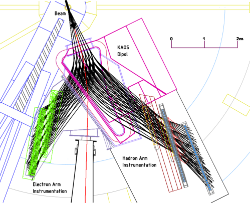
Fig. 5: Layout of the coming experiments with the Kaos spectrometer at zero degree scattering angle. Charged particles will be detected on both sides of the beam exit, ray-traced trajectories are shown by full lines. The instrumentation of the two spectrometer arms is indicated.

For the year 2011 elementary kaon electroproduction measurements with the Kaos spectrometer at zero degree scattering angle using the commissioned beam chicane and a first hypernuclear decay-pion spectroscopy experiment using the Kaos spectrometer as kaon tagger are planned. A feasibility study on the decay-pion spectroscopy in a single-arm measurement was performed in 2010.

- (1) K.H. Kaiser et al., Nucl. Instr. and Meth. in Phys. Res. A 593, 159 (2008)
- (2) R.A. Adelseck, B. Saghai, Phys. Rev. C 42, 108 (1990)
- (3) R.A. Williams, C.R. Ji, S.R. Cotanch, Phys. Rev. C 46, 1617 (1992)
- (4) C. Bennhold, H. Haberzettl, T. Mart, A new resonance in electroproduction: The (1895) and its electromagnetic form factors, arXiv:nucl-th/9909022 (1999)
- (5) T. Feuster, U. Mosel, Phys. Rev. C 59, 460 (1999)
- (6) E. Amaldi, S. Fubini, G. Furlan, Pion Electroproduction. Electroproduction at Low-Energy and Hadron Form-Factors, Vol. 83 of Springer Tracts in Mod. Phys. (Springer, Berlin, 1979)
- (7) T. Mart, C. Bennhold, H. Haberzettl, L. Tiator, An effective Lagrangian model for kaon photo- and electroproduction on the nucleon, online available at www.kph.uni-mainz.de/MAID/kaon/kaonmaid.html
- (8) T. Mart, C. Bennhold, Phys. Rev. C 61, 012201 (2000)
- (9) T. Mizutani, C. Fayard, G.H. Lamot, B. Saghai, Phys. Rev. C 58, 75 (1998)
- (10) P. Bydžovský, T. Mart, Phys. Rev. C 76, 065202 (2007)