The Bimodal Colors of Centaurs and Small Kuiper Belt Objects
Nuno Peixinho^1,2, Audrey Delsanti^3,4, Aurélie Guilbert-Lepoutre⁵, Ricardo Gafeira¹, and Pedro Lacerda^6
1 Center for Geophysics of the University of Coimbra, Av. Dr. Dias da Silva, 3000-134 Coimbra, Portugal [e-mail: peixinho@mat.uc.pt; gafeira@mat.uc.pt] ² Astronomical Observatory of the University of Coimbra, Almas de Freire, 3040-004 Coimbra, Portugal ³ Laboratoire d Astrophysique de Marseille, Université d’Aix-Marseille, CNRS, 38 rue Frédéric Joliot-Curie, 13388 Marseille, France [e-mail: Audrey.Delsanti@oamp.fr; Audrey.Delsanti@obspm.fr] ⁴ Observatoire de Paris, Site de Meudon, 5 place Jules Janssen, 92190 Meudon, France ⁵ UCLA, Department of Earth and Space Sciences, 595 Charles E. Young Drive East, Los Angeles CA 90095, USA [email: aguilbert@ucla.edu] ⁶ Queen’s University Belfast, Astrophysics Research Centre, Belfast BT7 1NN, United Kingdom [email: p.lacerda@qub.ac.uk] To appear in Astronomy & Astrophysics
Abstract. Ever since the very first photometric studies of Centaurs and Kuiper Belt Objects (KBOs) their visible color distribution has been controversial. That controversy gave rise to a prolific debate on the origin of the surface colors of these distant icy objects of the Solar System. Two different views attempt to interpret and explain the large variability of colors, hence surface composition. Are the colors mainly primordial and directly related to the formation region, or are they the result of surface evolution processes? To date, no mechanism has been found that successfully explains why Centaurs, which are escapees from the Kuiper Belt, exhibit two distinct color groups, whereas KBOs do not. In this letter, we readdress this issue using a carefully compiled set of $B-R$ colors and $H_{R}(\alpha)$ magnitudes (as proxy for size) for 253 objects, including data for 10 new small objects. We find that the bimodal behavior seen among Centaurs is a size related phenomenon, common to both Centaurs and small KBOs, i.e. independent of dynamical classification. Further, we find that large KBOs also exhibit a bimodal behavior of surface colors, albeit distinct from the small objects and strongly dependent on the ‘Haumea collisional family’ objects. When plotted in $B-R$, $H_{R}(\alpha)$ space, the colors of Centaurs and KBOs display a peculiar $\mathcal{N}$ shape. Key words. Kuiper belt: general

1 Introduction

Discovered just 20 years ago (Jewitt & Luu 1993), the Kuiper Belt holds a vast population of icy bodies orbiting the Sun beyond Neptune. Stored at very low temperatures ($\sim$30-50 K), the Kuiper Belt Objects (KBOs) are expected to be well-preserved fossil remnants of the solar system formation. Presently, $\sim$1600 KBOs have been identified and classified into several dynamical families (see Appendix A and Gladman et al. 2008, for a review). KBOs which dynamically evolve to become Jupiter Family Comets (JFCs) form a transient population, the Centaurs, with short-lived chaotic orbits between Jupiter and Neptune (Kowal et al. 1977; Fernandez 1980; Levison & Duncan 1997).

Between 1998 and 2003, we witnessed a debate on the surface colors of KBOs and Centaurs. One team used very accurate surface colors and detected that KBOs were separated into two distinct color groups (Tegler & Romanishin 1998, 2000, 2003). Other teams did not find evidence for such color bimodality (Barucci et al. 1999; Jewitt & Luu 2001; Hainaut & Delsanti 2002). Careful reanalysis of the data by Peixinho et al. (2003) indicated that only the Centaurs display bimodal colors, i.e. they are distributed in two distinct color groups, one with neutral solar-like colors, and one with very red colors. KBOs on the other hand exhibit a broad continuous color distribution, from neutral to very red, with no statistical evidence for a color gap between the extrema (Tegler et al. 2008, for a review).

The relevance of this controversy lays on two possible interpretations: i) KBOs and Centaurs are composed of intrinsically different objects, with distinct compositions, which probably formed at different locations of the protosolar disk, ii) KBOs and Centaurs are originally similar but evolutionary processes altered them differently, hence their color diversity. Most research focused on the latter hypothesis, offering little improvement on our understanding of the color distributions. Luu & Jewitt (1996) proposed that the competition between a reddening effect of irradiation of surface ices (Thompson et al. 1987) and a bluing effect due to collisional induced resurfacing of fresh, non-irradiated, ices might generate the observed surface colors. The same authors, however, rejected this model as being the primary cause of the color diversity, due to the lack of predicted rotational color variations (Jewitt & Luu 2001). Based on the same processes, Gil-Hutton (2002) proposed a more complex treatment of the irradiation process, by implying an intricate structure of differently irradiated subsurface layers. However, the collisional resurfacing effects became very hard to model, thus making it very hard to provide testable predictions. Later, Thébault & Doressoundiram (2003) showed that the collisional energies involved in different parts of the Kuiper Belt did not corroborate the possible link between surface colors and non-disruptive collisions.

Delsanti et al. (2004) refined the first-mentioned model by considering the effects of a possible cometary activity triggered by collisions, and a size/gravity-dependent resurfacing. Cometary activity can modify the surface properties through the creation of a neutral-color dust mantle. Jewitt (2002) suggested that this process could explain why no JFCs are found with the ultra-red surfaces seen in about half of the Centaurs. It has also been proposed that the sublimation loss of surface ice from a mixture with red materials may be sufficient to make the red material undetectable in the visible wavelengths (Grundy 2009). These might explain the Centaur color bimodality, as long as all were red when migrating inwards from the Kuiper Belt. Although promising, these models did not provide an explanation for the color bimodality of Centaurs, as they fail to reproduce the bluest colors observed and their frequency.

2 Motivation for This Work

We find it striking that the objects with both perihelion and semi-major axis between Jupiter and Neptune’s orbits, the Centaurs — by definition—, would display a different color distribution than physically and chemically similar objects with a semi-major axis slightly beyond Neptune’s orbit, as is the case for Scattered Disk Objects (SDOs), for instance, or any other KBOs. There is no evident physical consideration that would explain the apparently sudden ‘transition’ in surface color behavior (from bimodal to unimodal) precisely at Neptune’s orbital semi-major axis $a_{N}$ =30.07 AU. This difference between Centaurs and KBOs is particularly puzzling since there is neither a sharp dynamical separation between them, (the definition is somewhat arbitrary), nor a clearly identified family of KBOs in their origin. Although SDOs are frequently considered as the main source of Centaurs, Neptune Trojans, Plutinos, and Classical KBOs have been demonstrated as viable contributors (Horner & Lykawka 2010; Yu & Tremaine 1999; Volk & Malhotra 2008, respectivelly). Further, Centaurs possess short dynamical lifetimes of $\sim 5\cdot 10^{5}-3\cdot 10^{7}$ yr before being injected as JFCs or ejected again to the outer Solar System (Horner et al. 2004). If some surface evolution mechanism, dependent on heliocentric distance, is responsible for the bimodal behavior of Centaurs, it must be acting extremely fast such that no intermediate colors are ever seen among them. Besides surface color bimodality, the most distinctive characteristic of Centaurs compared to ‘other’ KBOs is their small size. Known KBOs are mostly larger than Centaurs, simply because they are more distant and thus smaller objects are harder to detect.

In this work, we address the issue of the color distributions of Centaurs and KBOs. We present new data on seven intrinsically faint (thus small) KBOs and three Centaurs, combined with a new compilation of 253 published $B-R$ colors, and available $m_{R}(1,1,\alpha)$ magnitudes, or $H_{R}(\alpha)$, i.e. absolute magnitude non-corrected from phase effects, and some identified spectral features. We study this large sample of colors (including objects from all dynamical families) versus absolute magnitude as a proxy for size, with the implicit assumption that surface colors are independent of dynamical classification. We present the most relevant results, found in $B-R$ vs. $H_{R}(\alpha)$ space.

3 Observations and Data Reduction

Observations of 7 KBOs and 1 Centaur were taken at the 8.2 m Subaru telescope, on 2008–07–02, using $0.^{\prime\prime}206/$pix FOCAS camera in imaging mode with $2\times 2$ binning (2 CCDs of $2048\times 4096$ pixels, Kashikawa et al. 2002). Weather was clear with seeing $\sim$$0.7^{\prime\prime}$. We used the University of Hawaii UH 2.2 m telescope, to observe 2 Centaurs on 2008–09–29, with the $0.^{\prime\prime}22/$pixel Tektronix $2048\times 2048$ pixels CCD camera. Weather was clear with seeing $\sim$$0.9^{\prime\prime}$. Both telescopes are on Mauna Kea, Hawaii, USA. Images from both instruments were processed using IRAF’s CCDRED package following the standard techniques of median bias subtraction and median flat-fielding normalization.

Table 1: Filters specifications

		8.2m Subaru			UH 2.2m
Filter		Wavelength (Å)			Wavelength (Å)
		Center	Width		Center	Width
B		4400	1080		4480	1077
R		6600	1170		6460	1245

Standard calibration was made observing Landolt standard stars (Landolt 1992) at different airmasses for each filter, obtaining the corresponding zeropoints, solving by non-linear least-square fits the transformation equations, directly in order of $R$ and $(B-R)$, using IRAF’s PHOTCAL package. The characteristics of the filters used on each telescope were essentially equal (Tab. 1). Subaru’s data was calibrated using Landolt standard stars: 107-612, PG1047+003B, 110-230, Mark A2, and 113-337, taken repeatedly at different airmasses. UH2.2m’s data was calibrated, analogously, using the stars: 92-410, 92-412, 94-401, 94-394, PG2213-006A and PG2213-006B. These stars have high photometric accuracy and colors close to those of the Sun. We have used the typical extinction values for Mauna Kea, $k_{B}=0.19$, and $k_{R}=0.09$ (Krisciunas et al. 1987, and CFHT Info Bulletin #19). All fits had residuals $rms<0.02$, which were added quadratically to the photometric error on each measurement. Targets were observed twice in B and twice in R bands, to avoid object trailing in one long exposure. Each two B or R exposures were co-added centered in the object, and also co-added centered on the background stars. The former were used to measure the object, the latter to compute the growth-curve correction. The time and airmass of observation were computed to the center of the total exposure. We applied growth-curve correction techniques to measure the target’s magnitudes using IRAF’s MKAPFILE task (for details, see Peixinho et al. 2004). Observation circumstances and results are shown in Table 2.

Table 2: Observational circumstances and photometric results of this work’s data

Object		Dyn. Class∗	Telescope	UT Date	$r$[AU]	$\Delta$[AU]	$\alpha[^{\circ}]$	R	B-R	$H_{R}(\alpha)$
(130391)	2000 JG81	2:1	Subaru	20080702UT07:24:58	34.073	34.817	1.2	23.12$\pm$0.03	1.42$\pm$0.06	7.75$\pm$0.06
(136120)	2003 LG7	3:1	Subaru	20080702UT09:42:53	32.815	33.659	1.0	23.54$\pm$0.05	1.27$\pm$0.09	8.32$\pm$0.05
(149560)	2003 QZ91	SDO	Subaru	20080702UT13:08:33	25.849	26.509	1.7	22.48$\pm$0.03	1.30$\pm$0.05	8.30$\pm$0.03
	2006 RJ103	Nep. Trojan	Subaru	20080702UT14:07:50	30.760	30.534	1.9	22.27$\pm$0.02	1.90$\pm$0.04	7.40$\pm$0.02
	2006 SQ372	SDO	Subaru	20080702UT11:45:34	23.650	24.287	1.9	21.55$\pm$0.02	1.78$\pm$0.03	7.71$\pm$0.05
	2007 JK43	SDO	Subaru	20080702UT08:08:13	23.113	23.766	1.9	20.73$\pm$0.02	1.40$\pm$0.03	7.03$\pm$0.02
	2007 NC7	SDO	Subaru	20080702UT11:30:49	20.090	20.916	1.7	21.19$\pm$0.02	1.28$\pm$0.03	8.07$\pm$0.02
(281371)	2008 FC76	Cent	Subaru	20080702UT11:13:05	11.119	11.793	3.8	19.79 $\pm$0.02	1.76$\pm$0.02	9.18$\pm$0.04
	2007 RH283	Cent	UH2.2m	20080929UT12:43:47	17.081	17.956	1.6	20.85 $\pm$0.03	1.20$\pm$0.05
	2007 RH283	Cent	UH2.2m	20080929UT12:57:51	17.081	17.956	1.6	20.90$\pm$0.03	1.28$\pm$0.06
	mean…								1.24$\pm$0.07	8.44$\pm$ 0.04
	2007 UM126	Cent	UH2.2m	20080929UT08:56:52	10.191	11.177	0.9	20.43$\pm$0.03	1.21$\pm$0.05
	2007 UM126	Cent	UH2.2m	20080929UT09:06:41	10.191	11.177	0.9	20.53$\pm$0.03	0.92$\pm$0.04
	2007 UM126	Cent	UH2.2m	20080929UT09:16:17	10.191	11.177	0.9	20.38$\pm$0.02	1.12$\pm$0.04
	mean…								1.08$\pm$0.10	10.16$\pm$0.04

4 Compilation of Data

We compiled the visible colors for 290 objects (KBOs, Centaurs, and Neptune Trojans) for which the absolute magnitude in R or V band was accessible (e.g. with individual magnitudes and observing date available), and surface spectra information for 48 objects, as published in the literature to date (Feb. 2012). We computed the absolute magnitude $H_{R}(\alpha)\equiv m_{R}(1,1,\alpha)=R-5\,log\,(r\cdot\Delta)$, where $R$ is the R-band magnitude, $r$ and $\Delta$ are the helio- and geocentric distances in AU, respectively. In this compilation, 253 objects have $B-R$ color available which is the focus of this paper (see Table A), and 48 have also spectral information. The description of the compilation method is presented in Appendix A. Sun-Object-Earth phase angles $\alpha$ are, typically, less than $1.5^{\circ}$ for KBOs and less than $4^{\circ}$ for Centaurs. Measurements of magnitude dependences on the phase angle for these objects, i.e. phase coefficients $\beta$[mag/$\,{}^{\circ}$], are scarce but, so far, do not show evidence for extreme variability presenting an average value of $\beta=0.11\pm 0.05$ (Belskaya et al. 2008). From the linear approximation $H_{R}(\alpha=0^{\circ})\approx H_{R}(\alpha)-\alpha\beta$, by not correcting the absolute magnitude from phase effects we are slightly overestimating it. We will deal with this issue in Sec. 5.

Recent works have shown that there is no strong correlation between object diameter $D$ and geometric albedo $p_{V}$, nor between geometric albedo $p_{V}$ and absolute magnitude $H_{R}$ (Stansberry et al. 2008; Santos-Sanz et al. 2012; Vilenius et al. 2012; Mommert et al. 2012). However, from the 74 diameter and albedo measurements of Centaurs and KBOs made using Herschel and/or Spitzer telescopes, published in the aforementioned works, we verify that $H_{R}$ and $D$ correlate very strongly with a Spearman-rank correlation of $\rho=-0.92^{+0.03}_{-0.02}$, with a significance level $SL\ll 0.01\%$ (error bars computed using bootstraps, for details see Doressoundiram et al. 2007). Consequently, absolute magnitude is a very good proxy for size.

5 An $\mathcal{N}$-shaped Doubly Bimodal Structure

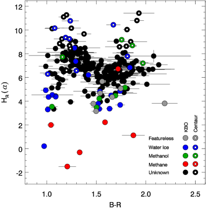
Figure 1: $B-R$ vs. $H_{R}(\alpha)$ plot of all 253 objects. KBOs are represented by solid circles and Centaurs by white dotted solid circles. Objects with $H_{R}(\alpha)\geqslant 6.8$ separate into two color groups with a ‘gap’ centered at $B-R\sim 1.60$. Objects with $H_{R}(\alpha)\leqslant 5.0$ also show statistical evidence for separation in two colors groups but with a ‘gap’ centered at $B-R\sim 1.25$. Objects spectra with known features of water ice, methane, methanol, and featureless spectra, are coded using colors as described in the legend. There is no obvious/clear connection between $B-R$ colors and the presence of spectral features.

In Fig. 1 we plot $R$-band absolute magnitude $H_{R}(\alpha)$ (proxy for object’s size) against $B-R$ color for all ($n=253$) objects in our database. The cloud of points forms a recognizable $\mathcal{N}$ shape with an apparent double bimodal structure in color. The smaller objects (upper part of the plot) show a bimodal $B-R$ distribution. Although apparently dominated by Centaurs, this bimodal distribution also includes KBOs of similar $H_{R}(\alpha)$, which suggests that the bimodal structure in $B-R$ color is a property of the smaller objects in general, regardless of their dynamical family. This bimodality appears do disappear for objects with $H_{R}(\alpha)\lesssim 7$ where the $B-R$ color distribution seems unimodal. Most interestingly, we note that towards the larger objects (lower part of the plot) the colors suggest the presence of another bimodal behavior, with the gap between the two groups shifted towards the blue with respect to the ‘small’ object bimodality. This new ‘large’ object bimodality is explicitly reported for the first time.

When performing hypotheses testing one should adopt a critical value of significance $\alpha$. The value $\alpha$ is the maximum probability (risk) we are willing to take in rejecting the null hypothesis $H_{0}$ (i.e. to claim no evidence for bimodality) when it is actually true (i.e. data is truly bimodal/multimodal) — also called type I error probability. Such value is often a source of debate, as the theories of hypotheses testing themselves (e.g. Lehmann 1993). The decision relies mostly whether the effects of a right or wrong decision are of practical importance or consequence. The paradigm is: by diminishing the probability of wrongly reject a null hypothesis (e.g. decide for bimodality when bimodality was not present in the parent population) we increase the probability of wrongly accepting the null hypothesis (i.e. deciding for unimodality when bimodality was in fact present), also called type II error probability, or risk factor $\beta$. Some authors and/or research fields, consider that there is only sufficient evidence against $H_{0}$ when the achieved significance level is $SL<0.3\%$, i.e. using $\alpha=0.3\%$ (the $3\sigma$ Gaussian probability), others require even $\alpha=0.0003\%$ ($6\sigma$). Such might be a criterion for rejection of $H_{0}$ but not a very useful ‘rating’ for the evidence against $H_{0}$, which is what we are implicitly doing. We rate the evidence against $H_{0}$ following a most common procedure in Statistics: $SL<5\%$ — reasonably strong evidence against $H_{0}$, $SL<2.5\%$ — strong evidence against $H_{0}$, and $SL<1\%$ — very strong evidence against $H_{0}$ (e.g. Efron & Tibshirani 1993), adding also the common procedure in Physics: $SL<0.3\%$ — clear evidence against $H_{0}$. Further, for better readability, throughout this work we may employ the abuse of language ‘evidence for bimodality’ instead of the statistically correct term ‘evidence against unimodality’.

Using the R software’s (version 2.14.1; R Development Core Team 2011) Dip Test package (Hartigan 1985; Hartigan & Hartigan 1985; Maechler 2011) we test the null hypothesis $H_{0}$: ‘the sample is consistent with an unimodal parent distribution’ over all objects in the $B-R$ vs. $H_{R}(\alpha)$ space, against the alternative hypothesis $H_{1}$: ‘the sample is not consistent with an unimodal parent distribution’ (hence it is bimodal or multimodal). The full sample, in spite of the apparent two spikes, shows no relevant evidence against color unimodality, neither with ($n=253$, $SL=17\%$) nor without ($n=224$, $SL=41\%$) Centaurs (see Fig. 2 a). The Centaur population ($n=29$) shows strong evidence against unimodality at $1.6\%$. Removing the 3 brightest Centaurs (with $H_{R}(\alpha)\gtrsim 6.6$) improves the significance to $0.3\%$. To refine the analysis and test different ranges in $H_{R}(\alpha)$ we ran the Dip Test on sub-samples using a running cutoff in $H_{R}(\alpha)$ that was shifted by 0.1 mag between consecutive tests.

Bimodal distribution of ‘small’ objects:

We performed iterative Dip Tests with a $H_{R:\,cut}$ starting at the maximum $H_{R}(\alpha)$ value, and decreasing in steps of 0.1 mag; in each iteration we run the test on those objects above the cutoff line (i.e. with $H_{R}(\alpha)\geqslant H_{R:\,cut}$). We stop shifting $H_{R:\,cut}$ when we detect the maximum of evidence against unimodality (i.e. a minimum of significance level, henceforth accepting the alternate hypothesis ‘the distribution is bimodal/multimodal’) Evidence for bimodality at significance levels better than $5\%$ start to be seen for objects with $H_{R}(\alpha)\geqslant 7.1$. This evidence peaks at a significance of $0.1\%$ for the $124$ faint objects with $H_{R}(\alpha)\geqslant 6.8$.

We propose that the visible surface color distribution of (non-active) icy bodies of the outer Solar System depends only on objects size, and is independent of their dynamical classification. No mechanism has yet been found to explain the color bimodality only for Centaurs. However, since such mechanism might exist even if not yet found, we re-analyze the sample removing the Centaurs. Naturally, the sampling of the smaller objects diminishes considerably, hence reducing the statistical significance against the null hypothesis (i.e. increases the probability of observing two groups on a purely random distribution of colors). Nonetheless, the $98$ remaining objects with $H_{R}(\alpha)\geqslant 6.8$ show evidence for bimodality at a significance level of $3.5\%$, reaching a significance minimum of $1.8\%$ for the $165$ objects with $H_{R}(\alpha)\geqslant 5.8$. In both cases the ‘gap’ is centered around $B-R\sim 1.60$ (see Figs. 1 and 2 b).

Bimodal distribution of ‘large’ objects:

We test the brightest part of the sample using a cutoff limit starting at the minimum $H_{R}(\alpha)$ value; we consider objects below the cutoff (i.e. brighter than $H_{R:\,cut}$) and shift it up in steps of 0.1 mag. We find very strong evidence against unimodality for objects with $H_{R}(\alpha)\lesssim 5.0$ ($SL=0.9\%$). Data still shows reasonably strong evidence against unimodality for objects up to $H_{R}(\alpha)\lesssim 5.6$. The ‘gap’ is located at $B-R\sim 1.25$. There are no Centaurs in this brightness range. Explicitly, evidence for ‘large’ objects bimodality has not been previously reported. (see Figs. 1 and 2 c). Removing from the sample the 7 objects belonging to the ‘Haumea collisional family’ (Brown et al. 2007b; Snodgrass et al. 2010), all clustered on the lower left ‘leg’ of the $\mathcal{N}$ shape, erases the statistical evidence against the null hypothesis, even if still suggestive to the eye. Therefore, with the present data sample, the ‘evidence for bimodality’ among bright KBOs cannot be stated as independent from the peculiar properties of the Haumea collisional family.

The ‘intermediate’ size continuum:

The 91 objects with $6.8>H_{R}(\alpha)>5.0$, which include 3 Centaurs, do not show evidence against a unimodal behavior ($SL=98.0\%$) even if a small gap seems suggestive to the eye (see Figs. 1 and 2 d). However, statistically, their inclusion in the fainter group does not decrease the significance below the ‘strong evidence against unimodality’, i.e. $SL=2.5\%$ (see Figs. 1 and 2 d). On the other hand, if added to the ‘large’ objects the statistical evidence for bimodality of ‘large’ objects does not hold.

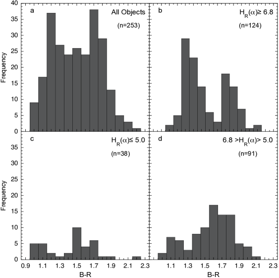
Figure 2: Histograms of $B-R$ colors from selected $H_{R}(\alpha)$ ranges: a) All the 253 objects. Taken globally do not exhibit statistical evidence for bimodality, which was known to exist among Centaurs. b) The 124 ‘small’ objects, with $H_{R}(\alpha)\geqslant 6.8$. Evidence for bimodal behavior is clear and still present when removing Centaurs. c) The 38 ‘large’ objects, with $H_{R}(\alpha)\leqslant 5.0$. A bimodal behavior is shown but it loses the statistical significance without the ‘Haumea collisional family’ objects. d) The 91 ‘intermediate’ size objects, $6.8>H_{R}(\alpha)>5.0$. Regardless of the apparent small gap at $B-R\sim 1.3$ there is no statistical evidence for two separate groups.

To check for the effects of non-correcting $H_{R}(\alpha)$ from phase angle effects we performed Monte-Carlo simulations. First, we compute all the possible $\alpha$ values and their probability distribution for an ‘average’ Centaur with semi-major axis $a=15$ AU. The maximum $\alpha$ is $3.8^{\circ}$ being the median value $3.2^{\circ}$. Analogously, we do the same for a KBO with $a=40$ AU. The maximum $\alpha$ is $1.4^{\circ}$ and the median value $1.2^{\circ}$. Therefore, on average, our absolute magnitudes might be overestimated by $\Delta H_{R}\approx 0.35$, for Centaurs, and by $\Delta H_{R}\approx 0.13$, for KBOs. Simulating 1000 ‘phase-corrected’ $H_{R}$ data-samples, following the probability distribution of the corresponding $\alpha$ angles did not alter any of the results obtained using simply $H_{R}(\alpha)$.

6 Interpretation

Our analysis shows that the $B-R$ colors of Centaurs and KBOs when plotted as a function of $H_{R}(\alpha)$ display an N-shaped, double bimodal behavior. The color distribution seems to depend on object size (intrinsic brightness) instead of dynamical family. Using the brightness-size-albedo relation $D_{km}=2\sqrt{\,2.24\cdot 10^{16}\cdot 10^{\,0.4\,(H_{R\,\odot}-H_{R})}/p_{R}}$, with solar $H_{R\,\odot}=-27.10$, the main issue is to choose a canonical geometric albedo value $p_{R}$. Recent works (Stansberry et al. 2008; Santos-Sanz et al. 2012; Vilenius et al. 2012; Mommert et al. 2012) show a wide range of values, for each dynamical family, in some cases far from the 0.04 value previously assumed from comet studies. As we need only a rough estimate of size ranges, we pick the average value of $p_{R}=0.09$. Using this parameter, objects with diameters $165\lesssim D_{km}\lesssim 380$ present a rather continuous range of B-R colors.

Visible and near-infrared (NIR) spectroscopy for about 75 bright objects (Barucci et al. 2011, for a review) also indicates that the surface compositions of KBOs and Centaurs is very diverse. The largest objects are coated in methane ice, while intermediate size objects display water-ice features, sometimes with traces of other volatiles. Small KBOs generally have featureless spectra. The presence of volatiles on the surface of an object may be related to its ability to retain them, i.e. to its size and temperature (Schaller & Brown 2007). It should also depend on the subsequent irradiation history (Brown et al. 2011). However no correlation can be made to date between visible colors and NIR spectral properties. For example, two objects of comparable size, Quaoar and Orcus, both exhibit water ice-dominated surfaces but have, respectively, very red and neutral visible colors (Delsanti et al. 2010).

Objects smaller than $\sim$100-150 km, including most of the known Centaurs, are believed to be fragments from the collision of larger objects (Pan & Sari 2005). Predicting the properties of these fragments is a complex task, but the field shows promising advances (for a review, see Leinhardt et al. 2008). An immediate hypothesis is that red and neutral objects are the only possible outcomes of a disruptive collision. Thermal evolution modeling suggests that KBOs, especially large ones, should have a layered structure, including some liquid water leading to a complete differentiation of the object (Merk & Prialnik 2006; Guilbert-Lepoutre et al. 2011). A catastrophic collision could result in the formation of fragments with very different properties, depending on whether they come from the core of the parent body, or its mantle, or some subsurface layers. However, our current knowledge of KBOs internal properties and evolution is still incipient to support or discard such an hypothesis. Besides, it is hard to understand why objects with $B-R\sim 1.6$ (in the gap of the small object’s bimodal distribution) should be inexistent. Maybe their relative number is so small compared to the neutral and red groups that we can hardly observe them, leading to another puzzling question. Research on these aspects should be encouraged, in particular the detection and measurement of many more small objects — KBOs and Centaurs — could help further constraining their color distribution and other properties. The objects in the ‘intermediate’ $H_{R}(\alpha)$ range ($6.8>H_{R}(\alpha)>5.0$) seem unimodally distributed in $B-R$ color; they might represent a transition phase between the two bimodal distributions. These medium-sized objects are probably too large to be remnants from disruptive collisions, and too small to have recently undergone cryovolcanic activity (they may not even be differentiated). They might, actually, represent the only group where the outcomes of the combined effects of different birthplaces, space weathering and thermal processing can be studied or analyzed.

The evidence for bimodal distribution among the largest objects is also puzzling. These are supposedly the best studied objects, yet the evidence for a bimodal distribution of their surface colors has never been reported. Nonetheless, when removing the 7 Haumea collisional family objects from our sample it no longer provides evidence against an unimodal distribution, even if apparent to the eye. This issue should be further analyzed when larger sampling is available.

In this work, we confirm that there is no noticeable link between the surface composition of an object and its visible colors. Objects hosting water ice are distributed both among large and small objects, and among red and blue ones. When it comes to volatiles such as methane (CH₄) or methanol (CH₃OH), we find that they are also distributed among all groups, although they might be more difficult to detect on small/fainter objects. We nonetheless find a cluster of featureless objects among the red group of large objects: these might represent the most irradiated/oldest surfaces in the overall population. Therefore, it seems that a simple explanation such as the model of atmospheric escape proposed by Schaller & Brown (2007) might not be sufficient to explain the colors and compositions of KBOs. The reason why they evolved in two different color groups can be very complex, and should involve different thermal, collisional, irradiation histories, on top of possible different birthplaces.

7 Summary

In this work we analyze the $B-R$ color distribution as a function of $H_{R}(\alpha)$ magnitude for 253 Centaurs and KBOs, including 10 new measurements, and with the information on their NIR spectral features. Using the known diameters, $D$, and albedos, $p_{V}$, of 74 of these objects we verify that $H_{R}$ and $D$ correlate very strongly ($\rho=-0.92^{+0.03}_{-0.02}$, $SL\ll 0.01\%$) validating $H_{R}$ as a good proxy for size. Further, through simulations, we show that not correcting $H_{R}(\alpha)$ to $H_{R}(\alpha=0^{\circ})$ does not change any of the global results. Our analysis shows:

1. The $B-R$ vs. $H_{R}(\alpha)$ color distribution is $\mathcal{N}$-shaped, evidencing that $B-R$ colors are probably dominated by a size effect independent from dynamical classification.

2. Small objects, including both KBOs and Centaurs, display a bimodal structure of $B-R$ colors at $0.1\%$ significance level (i.e. objects with $H_{R}(\alpha)\geqslant 6.8$, or $D_{km}\lesssim 165$, assuming $p_{R}=0.09$) with the ‘gap’ centered at $B-R\sim 1.60$. Removing Centaurs from the sample reduces greatly the sampling on small objects reducing also the significance of the result to $3.8\%$.

3. Large objects evidence also for a bimodal structure, with minimum significance of $0.9\%$, for $H_{R}(\alpha)\lesssim 5.0$ ($D_{km}\gtrsim 380$, assuming $p_{R}=0.09$), and color ‘gap’ centered at $B-R\sim 1.25$. Reasonable evidence for this bimodality starts when considering only objects with $H_{R}(\alpha)\lesssim 5.6$ ($D_{km}\gtrsim 290$) dropping below the critical $5\%$ when reaching $H_{R}(\alpha)\lesssim 4.4$ ($D_{km}\gtrsim 500$). However, this behavior seems dominated by the presence of 7 Haumea collisional family objects which ‘cluster’ at the lower left leg of the $\mathcal{N}$-shape. Once removed, there is no statistical evidence against compatibility with a random unimodal distribution for the larger KBOs.

4. Intermediate sized objects do not show incompatibility with a continuum of $B-R$ colors (i.e. $6.8>H_{R}(\alpha)>5.0$, or $165\lesssim D_{km}\lesssim 380$, assuming $p_{R}=0.09$). These objects seem too large to be remnants from disruptive collisions and too small to hold cryovolcanic activity. They might be the best targets to study the combined effects of different birthplaces, different space weathering, and different thermal processing. Further studies are encouraged.

5. Inspecting the NIR spectral properties against $B-R$ colors shows no obvious link between the colors and the chemical composition of the objects’ surfaces.

Appendix A Compiled Database

For each object, we compute the average color index from the different papers from data obtained simultaneously in B and R bands (e.g. contiguous observations within a same night). When individual R apparent magnitude and date is available, we compute the $H_{R}(\alpha)=R-5\,log\,(r\cdot\Delta)$, where $R$ is the R-band magnitude, $r$ and $\Delta$ are the helio- and geocentric distances at the time of observation in AU, respectively. When V and $V-R$ color is available, we derive an R and then $H_{R}(\alpha)$ value. We do not correct for the phase angle $\alpha$ effect as we need only a general estimation of the absolute magnitude for our complete sample. In addition, few objects have phase correction coefficient available in the literature, and no universally accepted canonical values per dynamical class can be strictly adopted. Table A presents the resulting values. This table includes also spectral information on the presence of water ice, methanol, methane, or confirmed featureless spectra, as available in the literature. We highlight only the cases with clear bands on the spectrum which were reported/confirmed by some other work.

There is no strict definition for the dynamical classes of Centaurs and KBOs. Roughly speaking: objects orbiting in mean motion resonances with Neptune are called ‘resonants’ (if located in the 1:1 resonance are also known as Neptune Trojans, and known as Plutinos if located in the 3:2 resonance); Centaurs are the objects with orbits between those of Jupiter and Neptune; Scattered Disk Objects (SDOs), are those within probable gravitational influence of Neptune; Detached KBOs, are those beyond past or future gravitational influence by Neptune; Classical KBOs , are those with rather circular orbits beyond Neptune and below the 2:1 resonance region (being called Hot if their orbital inclination is higher than $5^{\circ}$ or Cold if lower).

To determine the dynamical class we first gathered the orbital elements, with epoch 2011–12–05, from ‘The Asteroid Orbital Elements Database’, astorb.dat , maintained by the ‘Lowell Observatory’ based on astrometric observations by the ‘Minor Planet Center’. Then, using the particular classification scheme suggested by Lykawka & Mukai (2007), including their analysis of objects located in the mean motion resonances (MMR) with Neptune, dynamical class was determined following a 11 steps algorithm:

1. $q<a_{J}\Rightarrow$ Not analysed

2. in $1:1$ MMR with Neptune $\Rightarrow$ Neptune Trojan

3. in $3:2$ MMR with Neptune $\Rightarrow$ Plutino

4. in other MMR with Neptune $\Rightarrow$ Other Resonant

5. $q>a_{J}\wedge a<a_{N}\Rightarrow$ Centaur

6. $a_{J}<q<a_{N}\wedge a\geqslant a_{N}\Rightarrow$ Scattered Disk Object (SDO)

7. $a_{N}<q\leqslant 37\,AU\Rightarrow$ Scattered Disk Object (SDO)

8. $q\geqslant 40\,AU\wedge a\geqslant 48\,AU\Rightarrow$ Detached KBO (DKBO)

9. $37\,AU\leqslant q\leqslant 40\,AU\Rightarrow$ Scattered or Detached KBO (SDKBO)

10. $i<5^{\circ}\wedge\{\,[q\geqslant 37\,AU\wedge(37\,AU\leqslant a\leqslant 40\,AU)]\vee[q\geqslant 38\,AU\wedge(42\,AU\leqslant a\leqslant 48\,AU)]\,\}\Rightarrow$ Cold Classical KBO (cCKBO)

11. $i\geqslant 5^{\circ}\wedge q\geqslant 37\,AU\wedge(37\,AU\leqslant a\leqslant 48\,AU)\Rightarrow$ Hot Classical KBO (hCKBO)

being $q$ and $a$ the object’s perihelion and semi-major axis, respectively. Jupiter semi-major axis is $a_{J}$, and Neptune’s is $a_{N}$. Note that throughout the algorithm an object can be reclassified.

We are aware that there are more complex classification schemes, which may be more refined, but the boundaries between families do not change significantly. We chose this one for its computational simplicity.

References for the colors presented in Table A are : (1) Luu & Jewitt (1996); (2) Lazzaro et al. (1997); (3) Romon-Martin et al. (2003); (4) Romanishin et al. (1997); (5) Romon-Martin et al. (2002); (6) Tegler & Romanishin (1998); (7) Jewitt & Luu (2001); (8) Doressoundiram et al. (2002); (9) Tegler & Romanishin (2000); (10) Delsanti et al. (2001); (11) Tegler & Romanishin (1997); (12) Jewitt & Luu (1998); (13) Barucci et al. (1999); (14) Boehnhardt et al. (2001); (15) Doressoundiram et al. (2007); (16) Doressoundiram et al. (2001); (17) Green et al. (1997); (18) Boehnhardt et al. (2002); (19) Tegler & Romanishin (2003); (20) Hainaut et al. (2000); (21) Sheppard (2010); (22) Barucci et al. (2000); (23) Rabinowitz et al. (2008); (24) Tegler et al. http)//www.physics.nau.edu/ tegler/research/survey.htm; (25) Tegler et al. (2003); (26) Peixinho et al. (2001); (27) Trujillo & Brown (2002); (28) Peixinho et al. (2004); (29) Ferrin et al. (2001); (30) Doressoundiram et al. (2005b); (31) Santos-Sanz et al. (2009); (32) Dotto et al. (2003); (33) Fornasier et al. (2004); (34) Doressoundiram et al. (2005a); (35) Gulbis et al. (2006); (36) Rabinowitz et al. (2007); (37) Romanishin et al. (2010); (38) Rabinowitz et al. (2006); (39) Lacerda et al. (2008); (40) Snodgrass et al. (2010); (41) Sheppard & Trujillo (2006).

References for the spectral features indicated in Table A are: (a) Romon-Martin et al. (2003); (b) Cruikshank et al. (1998); (c) Kern et al. (2000); (d) Guilbert et al. (2009b); (e) Jewitt & Luu (2001); (f) Brown et al. (1999); (g) Barkume et al. (2008); (h) Guilbert et al. (2009a); (i) Barucci et al. (2011); (j) DeMeo et al. (2010); (k) Grundy et al. (2005); (l) Barucci et al. (2010); (m) Delsanti et al. (2010); (n) Pinilla-Alonso et al. (2009); (o) Merlin et al. (2009); (p) Brown et al. (2007a); (q) Schaller & Brown (2008).

[x]llccll Compilation of absolute magnitude $H_{R}(\alpha)$, $B-R$ colors, and spectral features used in this work

Object Dynamical Class $H_{R}(\alpha)$ $B-R$ Spectral features References

Table A cont’d

Object Dynamical Class $H_{R}(\alpha)$ $B-R$ Spectral features References

References: see Appendix A
(2060) Chiron Centaur 6.287$\pm$0.022 1.010$\pm$0.044 Water ice 1, 2, 3, a
(5145) Pholus Centaur 7.198$\pm$0.056 1.970$\pm$0.108 Methanol 4, b
(7066) Nessus Centaur 9.020$\pm$0.068 1.847$\pm$0.165 1
(8405) Asbolus Centaur 9.257$\pm$0.120 1.228$\pm$0.057 Water ice 4, 5, c
(10199) Chariklo Centaur 6.569$\pm$0.015 1.299$\pm$0.065 Water ice 6, 7, d
(10370) Hylonome Centaur 9.250$\pm$0.131 1.153$\pm$0.081 1, 6, 8
(15760) 1992 QB₁ Cold Classical 6.867$\pm$0.121 1.670$\pm$0.145 1, 7, 9
(15788) 1993 SB Plutino 8.032$\pm$0.122 1.276$\pm$0.100 7, 9, 10
(15789) 1993 SC Plutino 6.722$\pm$0.074 1.720$\pm$0.140 Methane 1, 7, 11, 12, e
(15810) 1994 JR₁ Plutino 6.867$\pm$0.077 1.610$\pm$0.216 13
(15820) 1994 TB Plutino 7.527$\pm$0.091 1.759$\pm$0.155 1, 7, 10, 11, 13
(15874) 1996 TL₆₆ Scattered Disk Object 5.131$\pm$0.144 1.113$\pm$0.070 6, 7, 12, 13, 14
(15875) 1996 TP₆₆ Plutino 6.953$\pm$0.071 1.678$\pm$0.123 6, 7, 12, 13, 14, 15
(15883) 1997 CR₂₉ Scattered Disk Object 7.076$\pm$0.135 1.260$\pm$0.128 7, 16
(16684) 1994 JQ₁ Cold Classical 6.618$\pm$0.117 1.738$\pm$0.120 17, 18, 19
(19255) 1994 VK₈ Cold Classical 7.016$\pm$0.163 1.680$\pm$0.067 9
(19299) 1996 SZ₄ Plutino 8.184$\pm$0.159 1.299$\pm$0.102 7, 9, 18
(19308) 1996 TO₆₆ Resonant (19:11) 4.530$\pm$0.044 1.056$\pm$0.210 Water ice 6, 7, 12, 13, 14, 20, 21, f
(19521) Chaos Hot Classical 4.442$\pm$0.069 1.558$\pm$0.062 8, 9, 10, 22
(20000) Varuna Hot Classical 3.345$\pm$0.059 1.530$\pm$0.036 Water ice 8, g
(20108) 1995 QZ₉ Plutino 7.889$\pm$0.399 1.400$\pm$0.050 9, This work
(24835) 1995 SM₅₅ Hot Classical 4.352$\pm$0.040 1.018$\pm$0.052 Water ice 8, 10, 14, 23, g
(24952) 1997 QJ₄ Plutino 7.389$\pm$0.114 1.104$\pm$0.104 7, 18
(24978) 1998 HJ₁₅₁ Cold Classical 7.008$\pm$0.050 1.820$\pm$0.042 19
(26181) 1996 GQ₂₁ Resonant (11:2) 4.467$\pm$0.090 1.693$\pm$0.079 Methanol 18, 24, g
(26308) 1998 SM₁₆₅ Resonant (2:1) 5.757$\pm$0.119 1.620$\pm$0.105 9, 10, 15
(26375) 1999 DE₉ Resonant (5:2) 4.810$\pm$0.046 1.536$\pm$0.056 Featureless 7, 8, 25, h
(28978) Ixion Scattered Disk Object 3.366$\pm$0.038 1.634$\pm$0.035 Water ice 8, h
(29981) 1999 TD₁₀ Scattered Disk Object 8.698$\pm$0.038 1.230$\pm$0.028 Water ice 8, g
(31824) Elatus Centaur 10.439$\pm$0.107 1.672$\pm$0.071 Water ice 8, 10, 26, g
(32532) Thereus Centaur 9.365$\pm$0.038 1.190$\pm$0.032 Water ice 25, h
(32929) 1995 QY₉ Plutino 7.489$\pm$0.126 1.160$\pm$0.150 1, 13
(33001) 1997 CU₂₉ Cold Classical 6.173$\pm$0.078 1.804$\pm$0.115 7, 16, 22, 27
(33128) 1998 BU₄₈ Scattered Disk Object 6.889$\pm$0.127 1.692$\pm$0.089 8, 10
(33340) 1998 VG₄₄ Plutino 6.292$\pm$0.077 1.511$\pm$0.055 8, 14, 16, 24
(35671) 1998 SN₁₆₅ Scattered Disk Object 5.431$\pm$0.068 1.123$\pm$0.082 7, 10, 16
(38083) Rhadamanthus Scattered Disk Object 7.432$\pm$0.063 1.177$\pm$0.109 18
(38084) 1999 HB₁₂ Resonant (5:2) 6.718$\pm$0.050 1.409$\pm$0.049 16, 25, 27, 28
(38628) Huya Plutino 4.674$\pm$0.099 1.539$\pm$0.062 Featureless 29, 7, 16, 18, g
(40314) 1999 KR₁₆ Scattered Disk Object 5.527$\pm$0.039 1.872$\pm$0.068 7, 18, 27
(42301) 2001 UR₁₆₃ Resonant (9:4) 3.812$\pm$0.109 2.190$\pm$0.130 Featureless 15, 30, 31, g
(42355) Typhon Scattered Disk Object 7.358$\pm$0.076 1.292$\pm$0.071 Water ice 25, 28, h
(44594) 1999 OX₃ Scattered Disk Object 6.835$\pm$0.078 1.839$\pm$0.087 Water ice 8, 9, 10, 15, 21, 30, i
(47171) 1999 TC₃₆ Plutino 4.851$\pm$0.054 1.740$\pm$0.049 Water ice 10, 16, 25, 32, h
(47932) 2000 GN₁₇₁ Plutino 5.666$\pm$0.090 1.559$\pm$0.066 Featureless 18, 24, h
(48639) 1995 TL₈ Detached KBO 4.667$\pm$0.091 1.693$\pm$0.217 8, 10, 21
(49036) Pelion Centaur 10.157$\pm$0.112 1.248$\pm$0.096 9, 18
(50000) Quaoar Hot Classical 2.220$\pm$0.029 1.588$\pm$0.021 Methane 25, 33, h
(52747) 1998 HM₁₅₁ Cold Classical 7.417$\pm$0.100 1.550$\pm$0.103 19
(52872) Okyrhoe Centaur 10.775$\pm$0.078 1.237$\pm$0.086 Water ice 10, 16, 32, g
(52975) Cyllarus Centaur 8.634$\pm$0.101 1.803$\pm$0.102 8, 10, 14, 25
(53311) Deucalion Cold Classical 6.662$\pm$0.060 2.030$\pm$0.160 27
(54598) Bienor Centaur 7.727$\pm$0.077 1.158$\pm$0.075 Methanol 8, 10, 15, h
(55565) 2002 AW₁₉₇ Hot Classical 3.156$\pm$0.059 1.498$\pm$0.044 Featureless 24, 33, 34, h
(55576) Amycus Centaur 7.789$\pm$0.042 1.814$\pm$0.044 Water ic 24, 28, 33, 34, i
(55636) 2002 TX₃₀₀ Hot Classical 3.296$\pm$0.047 1.010$\pm$0.028 Water ice 25, 30, q
(55637) 2002 UX₂₅ Scattered Disk Object 3.486$\pm$0.084 1.502$\pm$0.052 Water ice 24, 31, g
(55638) 2002 VE₉₅ Plutino 5.143$\pm$0.062 1.790$\pm$0.040 Methanol 24, g
(58534) Logos Cold Classical 6.759$\pm$0.181 1.653$\pm$0.150 7, 22
(59358) 1999 CL₁₅₈ Scattered Disk Object 6.653$\pm$0.090 1.190$\pm$0.072 8
(60454) 2000 CH₁₀₅ Cold Classical 6.363$\pm$0.077 1.699$\pm$0.083 28
(60458) 2000 CM₁₁₄ Scattered Disk Object 6.954$\pm$0.044 1.240$\pm$0.040 25
(60558) Echeclus Centaur 9.669$\pm$0.090 1.376$\pm$0.072 18, 24
(60608) 2000 EE₁₇₃ Scattered Disk Object 8.028$\pm$0.107 1.164$\pm$0.032 18, 25
(60620) 2000 FD₈ Resonant (7:4) 6.344$\pm$0.061 1.806$\pm$0.113 18, 28
(60621) 2000 FE₈ Resonant (5:2) 6.510$\pm$0.062 1.230$\pm$0.027 8, 25
(63252) 2001 BL₄₁ Centaur 11.273$\pm$0.065 1.199$\pm$0.045 25, 28
(65489) Ceto Scattered Disk Object 6.205$\pm$0.060 1.420$\pm$0.040 Water ice 25, g
(66452) 1999 OF₄ Cold Classical 6.255$\pm$0.090 1.830$\pm$0.095 28
(66652) Borasisi Cold Classical 5.420$\pm$0.051 1.610$\pm$0.050 16, 35
(69986) 1998 WW₂₄ Plutino 7.964$\pm$0.096 1.235$\pm$0.152 8, 28
(69988) 1998 WA₃₁ Resonant (5:2) 7.303$\pm$0.149 1.412$\pm$0.127 28
(69990) 1998 WU₃₁ Plutino 7.988$\pm$0.200 1.225$\pm$0.086 28
(73480) 2002 PN₃₄ Scattered Disk Object 8.487$\pm$0.046 1.280$\pm$0.020 Water ice 25, j
(79360) 1997 CS₂₉ Cold Classical 5.068$\pm$0.085 1.746$\pm$0.077 Featureless 6, 7, 14, 22, k
(79978) 1999 CC₁₅₈ Resonant (12:5) 5.409$\pm$0.091 1.566$\pm$0.100 8, 10, 24
(79983) 1999 DF₉ Hot Classical 5.797$\pm$0.110 1.630$\pm$0.078 8
(80806) 2000 CM₁₀₅ Cold Classical 6.302$\pm$0.030 1.980$\pm$0.230 27
(82075) 2000 YW₁₃₄ Resonant (8:3) 4.429$\pm$0.064 1.417$\pm$0.077 21, 25, 28, 30, 31
(82155) 2001 FZ₁₇₃ Scattered Disk Object 5.811$\pm$0.027 1.418$\pm$0.030 25, 28
(82158) 2001 FP₁₈₅ Scattered Disk Object 5.940$\pm$0.053 1.402$\pm$0.055 25, 30
(83982) Crantor Centaur 8.693$\pm$0.057 1.864$\pm$0.044 Methanol 25, 28, 33, 34, h
(84522) 2002 TC₃₀₂ Scattered or Detached KBO 3.682$\pm$0.067 1.741$\pm$0.048 Water ice 21, 24, 31, g
(84719) 2002 VR₁₂₈ Plutino 5.005$\pm$0.040 1.540$\pm$0.040 24
(84922) 2003 VS₂ Plutino 3.794$\pm$0.070 1.520$\pm$0.030 Water ice 24, g
(85633) 1998 KR₆₅ Cold Classical 6.599$\pm$0.073 1.727$\pm$0.144 18, 19
(86047) 1999 OY₃ Scattered Disk Object 6.293$\pm$0.055 1.055$\pm$0.050 8, 9, 18
(86177) 1999 RY₂₁₅ Scattered Disk Object 6.736$\pm$0.114 1.151$\pm$0.183 16, 18
(87269) 2000 OO₆₇ Scattered Disk Object 9.057$\pm$0.170 1.702$\pm$0.092 21, 25
(87555) 2000 QB₂₄₃ Scattered Disk Object 8.439$\pm$0.119 1.088$\pm$0.094 15, 28
(88269) 2001 KF₇₇ Centaur 10.038$\pm$0.020 1.810$\pm$0.040 25
(90377) Sedna Detached KBO 1.120$\pm$0.088 1.874$\pm$0.115 Methane21, 24, 36, l
(90482) Orcus Scattered Disk Object 1.991$\pm$0.054 1.042$\pm$0.037 Methane 24, 36, m
(90568) 2004 GV₉ Hot Classical 3.786$\pm$0.080 1.470$\pm$0.040 Featureless 24, h
(91133) 1998 HK₁₅₁ Plutino 6.937$\pm$0.076 1.240$\pm$0.064 8, 16
(91205) 1998 US₄₃ Plutino 7.852$\pm$0.050 1.185$\pm$0.102 28
(91554) 1999 RZ₂₁₅ Scattered Disk Object 8.072$\pm$0.079 1.346$\pm$0.132 18
(95626) 2002 GZ₃₂ Centaur 6.603$\pm$0.131 1.199$\pm$0.075 25, 30, 33
(118228) 1996 TQ₆₆ Plutino 7.245$\pm$0.195 1.881$\pm$0.144 6, 7
(118378) 1999 HT₁₁ Resonant (7:4) 6.906$\pm$0.040 1.830$\pm$0.100 27
(118379) 1999 HC₁₂ Scattered Disk Object 7.611$\pm$0.170 1.384$\pm$0.214 18
(118702) 2000 OM₆₇ Scattered or Detached KBO 7.075$\pm$0.036 1.290$\pm$0.040 21
(119068) 2001 KC₇₇ Resonant (5:2) 6.822$\pm$0.030 1.470$\pm$0.010 25
(119070) 2001 KP₇₇ Resonant (7:4) 6.873$\pm$0.305 1.720$\pm$0.319 28, 30
(119315) 2001 SQ₇₃ Centaur 8.857$\pm$0.069 1.130$\pm$0.020 25, 31
(119473) 2001 UO₁₈ Plutino 7.804$\pm$0.506 2.079$\pm$0.376 30
(119878) 2002 CY₂₂₄ Resonant (12:5) 5.871$\pm$0.056 1.680$\pm$0.100 31
(119951) 2002 KX₁₄ Scattered Disk Object 4.349$\pm$0.124 1.660$\pm$0.040 Featureless 24, 37, h
(120061) 2003 CO₁ Centaur 9.134$\pm$0.140 1.240$\pm$0.040 25, 27
(120132) 2003 FY₁₂₈ Scattered Disk Object 4.486$\pm$0.053 1.650$\pm$0.020 Water ice 21,g
(120181) 2003 UR₂₉₂ Scattered Disk Object 7.093$\pm$0.100 1.690$\pm$0.080 24
(120216) 2004 EW₉₅ Plutino 6.309$\pm$0.050 1.080$\pm$0.030 24
(121725) 1999 XX₁₄₃ Centaur 8.586$\pm$0.096 1.734$\pm$0.145 8, 28
(126619) 2002 CX₁₅₄ Scattered or Detached KBO 7.178$\pm$0.075 1.470$\pm$0.128 31
(127546) 2002 XU₉₃ Scattered Disk Object 7.942$\pm$0.019 1.200$\pm$0.020 21
(129772) 1999 HR₁₁ Resonant (7:4) 7.172$\pm$0.150 1.450$\pm$0.156 16
(130391) 2000 JG₈₁ Resonant (2:1) 7.748$\pm$0.056 1.417$\pm$0.060 This work
(134860) 2000 OJ₆₇ Cold Classical 6.001$\pm$0.120 1.720$\pm$0.078 8
(135182) 2001 QT₃₂₂ Scattered Disk Object 7.752$\pm$0.320 1.240$\pm$0.060 37
(136108) Haumea Resonant(12:7) 0.205$\pm$0.011 0.973$\pm$0.024 Water ice 38, 39, n
(136120) 2003 LG₇ Resonant (3:1) 8.322$\pm$0.049 1.271$\pm$0.091 This work
(136199) Eris Scattered or Detached KBO -1.511$\pm$0.033 1.207$\pm$0.088 Methane 24, 36, o
(136204) 2003 WL₇ Centaur 8.670$\pm$0.070 1.230$\pm$0.040 24
(136472) Makemake Hot Classical -0.317$\pm$0.024 1.332$\pm$0.029 Methane 36,p
(137294) 1999 RE₂₁₅ Cold Classical 6.091$\pm$0.073 1.700$\pm$0.148 18
(137295) 1999 RB₂₁₆ Resonant (2:1) 7.668$\pm$0.096 1.419$\pm$0.142 18
(138537) 2000 OK₆₇ Cold Classical 6.093$\pm$0.083 1.540$\pm$0.094 8
(144897) 2004 UX₁₀ Hot Classical 4.216$\pm$0.087 1.530$\pm$0.020 Methanol 37, i
(145480) 2005 TB₁₉₀ Detached KBO 3.949$\pm$0.085 1.540$\pm$0.030 21
(148209) 2000 CR₁₀₅ Detached KBO 6.191$\pm$0.073 1.273$\pm$0.068 21, 25
(148780) Altjira Hot Classical 5.885$\pm$0.320 1.640$\pm$0.170 30
(149560) 2003 QZ₉₁ Scattered Disk Object 8.302$\pm$0.028 1.305$\pm$0.048 This work
(168703) 2000 GP₁₈₃ Scattered Disk Object 5.795$\pm$0.061 1.160$\pm$0.057 8
(181708) 1993 FW Hot Classical 6.572$\pm$0.105 1.625$\pm$0.110 1, 17, 19, 22
(181855) 1998 WT₃₁ Hot Classical 7.443$\pm$0.079 1.247$\pm$0.140 28, 40
(181867) 1999 CV₁₁₈ Resonant (7:3)? 7.067$\pm$0.163 2.130$\pm$0.090 27
(181868) 1999 CG₁₁₉ Scattered Disk Object 7.004$\pm$0.040 1.530$\pm$0.080 27
(181871) 1999 CO₁₅₃ Cold Classical 6.607$\pm$0.030 1.940$\pm$0.090 27
(181874) 1999 HW₁₁ Scattered or Detached KBO 6.706$\pm$0.062 1.323$\pm$0.043 21, 27
(182397) 2001 QW₂₉₇ Resonant (9:4) 6.660$\pm$0.064 1.600$\pm$0.070 21
(182934) 2002 GJ₃₂ Hot Classical 5.469$\pm$0.187 1.678$\pm$0.261 30, 31
1993 RO Plutino 8.492$\pm$0.113 1.385$\pm$0.154 1, 9
1994 EV₃ Cold Classical 7.110$\pm$0.072 1.732$\pm$0.167 1, 18, 27
1994 TA Centaur 11.421$\pm$0.126 1.930$\pm$0.155 9, 7
1995 HM₅ Plutino 7.849$\pm$0.109 1.010$\pm$0.192 6, 22
1995 WY₂ Cold Classical 6.864$\pm$0.110 1.655$\pm$0.278 1, 7
1996 RQ₂₀ Hot Classical 6.903$\pm$0.092 1.523$\pm$0.156 7, 10
1996 RR₂₀ Plutino 6.622$\pm$0.143 1.868$\pm$0.130 7, 9, 18
1996 TK₆₆ Cold Classical 6.190$\pm$0.116 1.666$\pm$0.088 7, 8, 9
1996 TS₆₆ Hot Classical 5.947$\pm$0.130 1.665$\pm$0.157 6, 7, 12
1997 CV₂₉ Hot Classical 7.154$\pm$0.030 1.860$\pm$0.022 19
1997 QH₄ Hot Classical 6.996$\pm$0.136 1.731$\pm$0.168 7, 9, 10, 18
1997 RT₅ Hot Classical 7.117$\pm$0.140 1.549$\pm$0.162 18
1997 SZ₁₀ Resonant (2:1) 8.100$\pm$0.104 1.790$\pm$0.085 9
1998 FS₁₄₄ Hot Classical 6.717$\pm$0.105 1.516$\pm$0.057 19, 22
1998 HL₁₅₁ Hot Classical 8.120$\pm$0.149 1.190$\pm$0.284 27, 40
1998 KG₆₂ Cold Classical 6.125$\pm$0.110 1.602$\pm$0.158 16, 18
1998 KS₆₅ Cold Classical 7.166$\pm$0.040 1.730$\pm$0.045 19
1998 UR₄₃ Plutino 8.083$\pm$0.132 1.390$\pm$0.113 10
1998 WS₃₁ Plutino 7.952$\pm$0.186 1.315$\pm$0.075 28
1998 WV₂₄ Cold Classical 7.126$\pm$0.067 1.270$\pm$0.032 9
1998 WV₃₁ Plutino 7.627$\pm$0.069 1.349$\pm$0.096 10, 28
1998 WX₂₄ Cold Classical 6.241$\pm$0.099 1.790$\pm$0.071 9
1998 WZ₃₁ Plutino 8.044$\pm$0.102 1.263$\pm$0.089 28
1998 XY₉₅ Scattered or Detached KBO 6.438$\pm$0.143 1.580$\pm$0.212 14
1999 CB₁₁₉ Hot Classical 6.740$\pm$0.050 1.926$\pm$0.095 28
1999 CD₁₅₈ Resonant (7:4) 4.837$\pm$0.111 1.384$\pm$0.116 8, 10, 40
1999 CF₁₁₉ Scattered or Detached KBO 6.982$\pm$0.084 1.424$\pm$0.072 27, 25
1999 CJ₁₁₉ Cold Classical 6.695$\pm$0.210 2.070$\pm$0.220 27
1999 CM₁₁₉ Cold Classical 7.356$\pm$0.060 1.780$\pm$0.170 27
1999 CQ₁₃₃ Hot Classical 6.682$\pm$0.050 1.350$\pm$0.070 27
1999 CX₁₃₁ Resonant (5:3) 6.914$\pm$0.087 1.637$\pm$0.118 28
1999 GS₄₆ Hot Classical 6.230$\pm$0.020 1.760$\pm$0.070 27
1999 HS₁₁ Cold Classical 6.344$\pm$0.081 1.845$\pm$0.099 16, 19, 28, 35
1999 HV₁₁ Cold Classical 7.003$\pm$0.050 1.700$\pm$0.063 19
1999 JD₁₃₂ Hot Classical 5.983$\pm$0.020 1.590$\pm$0.090 27
1999 OE₄ Cold Classical 6.887$\pm$0.193 1.832$\pm$0.147 28
1999 OJ₄ Cold Classical 6.899$\pm$0.060 1.675$\pm$0.077 28
1999 OM₄ Cold Classical 7.521$\pm$0.100 1.739$\pm$0.170 18
1999 RJ₂₁₅ Scattered Disk Object 7.881$\pm$0.103 1.221$\pm$0.175 18
1999 RX₂₁₄ Cold Classical 6.385$\pm$0.050 1.647$\pm$0.070 28
1999 RY₂₁₄ Hot Classical 7.006$\pm$0.040 1.258$\pm$0.085 28
1999 TR₁₁ Plutino 8.063$\pm$0.140 1.770$\pm$0.106 9
2000 AF₂₅₅ Scattered Disk Object 5.682$\pm$0.030 1.780$\pm$0.060 27
2000 CG₁₀₅ Hot Classical 6.469$\pm$0.293 1.170$\pm$0.170 27, 40
2000 CJ₁₀₅ Hot Classical 5.687$\pm$0.066 1.760$\pm$0.106 31
2000 CL₁₀₄ Cold Classical 6.394$\pm$0.086 1.851$\pm$0.192 18
2000 CL₁₀₅ Cold Classical 6.761$\pm$0.060 1.520$\pm$0.090 27
2000 CN₁₀₅ Cold Classical 5.286$\pm$0.160 1.720$\pm$0.128 31
2000 CO₁₀₅ Hot Classical 5.619$\pm$0.124 1.520$\pm$0.180 27
2000 CQ₁₀₅ Scattered Disk Object 5.996$\pm$0.054 1.107$\pm$0.043 25, 28
2000 FS₅₃ Cold Classical 7.165$\pm$0.124 1.786$\pm$0.095 19, 27
2000 FZ₅₃ Centaur 11.103$\pm$0.165 1.170$\pm$0.050 25
2000 KK₄ Hot Classical 5.982$\pm$0.103 1.550$\pm$0.050 19
2000 PE₃₀ Scattered Disk Object 5.867$\pm$0.110 1.132$\pm$0.084 15, 16, 21
2000 YB₂ Scattered Disk Object 6.436$\pm$0.084 1.500$\pm$0.134 31
2001 FM₁₉₄ Scattered Disk Object 7.453$\pm$0.159 1.190$\pm$0.040 25
2001 HY₆₅ Hot Classical 6.041$\pm$0.064 1.510$\pm$0.092 31
2001 HZ₅₈ Cold Classical 6.158$\pm$0.053 1.640$\pm$0.085 31
2001 KA₇₇ Hot Classical 5.050$\pm$0.089 1.812$\pm$0.122 8, 28, 30
2001 KB₇₇ Plutino 7.349$\pm$0.078 1.390$\pm$0.130 24
2001 KD₇₇ Plutino 5.928$\pm$0.096 1.763$\pm$0.060 8, 28
2001 KG₇₇ Scattered Disk Object 8.340$\pm$0.120 1.240$\pm$0.070 25
2001 KY₇₆ Plutino 6.689$\pm$0.380 1.960$\pm$0.291 30
2001 QC₂₉₈ Hot Classical 6.381$\pm$0.174 1.030$\pm$0.098 31
2001 QD₂₉₈ Hot Classical 6.185$\pm$0.170 1.640$\pm$0.158 30
2001 QF₂₉₈ Plutino 5.119$\pm$0.118 1.051$\pm$0.085 15, 24, 30
2001 QR₃₂₂ Neptune Trojan 7.828$\pm$0.010 1.260$\pm$0.036 41
2001 QX₃₂₂ Scattered Disk Object 6.144$\pm$0.146 1.752$\pm$0.280 25, 31
2001 QY₂₉₇ Cold Classical 5.151$\pm$0.231 1.561$\pm$0.177 15, 30, 35
2001 RZ₁₄₃ Cold Classical 6.241$\pm$0.123 1.590$\pm$0.191 31
2001 XZ₂₅₅ Centaur 10.800$\pm$0.080 1.910$\pm$0.070 25
2002 DH₅ Centaur 10.115$\pm$0.100 1.054$\pm$0.075 28
2002 GB₃₂ Scattered Disk Object 7.638$\pm$0.019 1.390$\pm$0.020 21
2002 GF₃₂ Plutino 5.973$\pm$0.210 1.765$\pm$0.134 30
2002 GH₃₂ Hot Classical 6.098$\pm$0.201 1.509$\pm$0.160 30, 31
2002 GP₃₂ Resonant (5:2) 6.580$\pm$0.162 1.386$\pm$0.162 30, 35
2002 GV₃₂ Plutino 6.886$\pm$0.199 1.860$\pm$0.122 30
2002 MS₄ Resonant (18:11) 3.333$\pm$0.040 1.070$\pm$0.040 24
2002 VT₁₃₀ Cold Classical 5.426$\pm$0.092 2.010$\pm$0.233 31
2002 XV₉₃ Plutino 4.434$\pm$0.040 1.090$\pm$0.030 24
2003 AZ₈₄ Plutino 3.537$\pm$0.053 1.052$\pm$0.057 Methanol 24, 31, 33, h
2003 FZ₁₂₉ Scattered or Detached KBO 6.983$\pm$0.038 1.320$\pm$0.040 21
2003 HB₅₇ Scattered or Detached KBO 7.389$\pm$0.028 1.310$\pm$0.030 21
2003 QA₉₂ Scattered Disk Object 6.367$\pm$0.240 1.670$\pm$0.020 37
2003 QK₉₁ Scattered or Detached KBO 6.966$\pm$0.036 1.370$\pm$0.040 21
2003 QQ₉₁ Scattered Disk Object 7.624$\pm$0.280 1.180$\pm$0.050 37
2003 QW₉₀ Hot Classical 4.730$\pm$0.057 1.780$\pm$0.092 31
2003 TH₅₈ Plutino 6.940$\pm$0.056 0.990$\pm$0.071 40
2003 UZ₁₁₇ Hot Classical 4.920$\pm$0.083 0.990$\pm$0.050 Water ice 24, q
2003 YL₁₇₉ Cold Classical 7.482$\pm$0.300 1.260$\pm$0.090 37
2004 OJ₁₄ Scattered or Detached KBO 6.991$\pm$0.028 1.420$\pm$0.030 21
2004 UP₁₀ Neptune Trojan 8.651$\pm$0.030 1.160$\pm$0.064 41
2004 XR₁₉₀ Detached KBO 3.937$\pm$0.036 1.240$\pm$0.040 21
2005 CB₇₉ Hot Classical 4.375$\pm$0.028 1.090$\pm$0.028 Water ice 40, q
2005 EO₂₉₇ Resonant (3:1) 7.221$\pm$0.047 1.320$\pm$0.050 21
2005 GE₁₈₇ Plutino 7.192$\pm$0.097 1.740$\pm$0.112 40
2005 PU₂₁ Scattered Disk Object 6.091$\pm$0.019 1.790$\pm$0.020 21
2005 SD₂₇₈ Scattered or Detached KBO 5.915$\pm$0.019 1.530$\pm$0.020 21
2005 TN₅₃ Neptune Trojan 9.027$\pm$0.040 1.290$\pm$0.106 41
2005 TO₇₄ Neptune Trojan 8.426$\pm$0.030 1.340$\pm$0.078 41
2006 RJ₁₀₃ Neptune Trojan 7.400$\pm$0.023 1.903$\pm$0.044 This work
2006 SQ₃₇₂ Scattered Disk Object 7.709$\pm$0.049 1.712$\pm$0.093 21, This work
2007 JJ₄₃ Hot Classical 4.044$\pm$0.019 1.610$\pm$0.020 21
2007 JK₄₃ Scattered Disk Object 7.028$\pm$0.017 1.400$\pm$0.027 This work
2007 NC₇ Scattered Disk Object 8.068$\pm$0.018 1.282$\pm$0.028 This work
2007 RH₂₈₃ Centaur 8.435$\pm$0.039 1.237$\pm$0.069 This work
2007 TG₄₂₂ Scattered Disk Object 6.186$\pm$0.010 1.390$\pm$0.040 21
2007 UM₁₂₆ Centaur 10.161$\pm$0.042 1.080$\pm$0.096 Water ice This work, i
2007 VJ₃₀₅ Scattered Disk Object 6.713$\pm$0.028 1.440$\pm$0.030 21
2008 FC₇₆ Centaur 9.181$\pm$0.039 1.756$\pm$0.024 Methanol This work, i
2008 KV₄₂ Scattered Disk Object 8.564$\pm$0.056 1.290$\pm$0.060 21
2008 OG₁₉ Scattered or Detached KBO 4.612$\pm$0.013 1.470$\pm$0.010 21