Nonlinear stability of mKdV breathers

Abstract.

Breather solutions of the modified Korteweg-de Vries equation are shown to be globally stable in a natural $H^{2}$ topology. Our proof introduces a new Lyapunov functional, at the $H^{2}$ level, which allows to describe the dynamics of small perturbations, including oscillations induced by the periodicity of the solution, as well as a direct control of the corresponding instability modes. In particular, degenerate directions are controlled using low-regularity conservation laws.

1. Introduction

This paper deals with the nonlinear stability of breathers of the focusing, modified Korteweg-de Vries (mKdV) equation

$$u_{t}+(u_{xx}+u^{3})_{x}=0.$$ (1.1)

Here $u=u(t,x)$ is a real-valued function, and $(t,x)\in\mathbb{R}^{2}$. The equation above is a well known completely integrable model [14, 2, 21], with infinitely many conserved quantities, and a suitable Lax-pair formulation. The Inverse Scattering Theory has been applied by many authors in order to describe the behavior of solutions in generality, see e.g. [2, 21] and references therein.

Solutions $u(t,x)$ of (1.1) are invariant under space and time translations, and under suitable scaling properties. Indeed, for any $t_{0},x_{0}\in\mathbb{R}$, and $c>0$, both $u(t-t_{0},x-x_{0})$ and $c^{1/2}u(c^{3/2}t,c^{1/2}x)$ are solutions of (1.1). Finally, if $u(t,x)$ is a solution of (1.1), then $u(-t,-x)$ and $-u(t,x)$ are also solutions.

On the other hand, standard conservation laws for (1.1) at the $H^{1}$-level are the mass

$$M[u](t):=\frac{1}{2}\int_{\mathbb{R}}u^{2}(t,x)dx=M[u](0),$$ (1.2)

and energy

$$E[u](t):=\frac{1}{2}\int_{\mathbb{R}}u_{x}^{2}(t,x)dx-\frac{1}{4}\int_{\mathbb{R}}u^{4}(t,x)dx=E[u](0).$$ (1.3)

A satisfactory Cauchy theory is also present at such a level of regularity or even lower, see e.g. Kenig-Ponce-Vega [19], and Colliander et al. [12]. From the Inverse Scattering Theory, the evolution of a rapidly decaying initial data can be described by purely algebraic methods. Solutions are shown to decompose into a very particular set of solutions (see Schuur [34]), described in detail below.

Indeed, equation (1.1) is also important because of the existence of solitary wave solutions called solitons. These profiles are often regarded as minimizers of a constrained functional in the $H^{1}$-topology. For example, mKdV (1.1) has solitons of the form

$$u(t,x)=Q_{c}(x-ct),\quad Q_{c}(s):=\sqrt{c}Q(\sqrt{c}s),\quad c>0,$$ (1.4)

with

$$Q(s):=\frac{\sqrt{2}}{\cosh(s)}=2\sqrt{2}\partial_{s}[\arctan(e^{s})].$$

By replacing (1.4) in (1.1), one has that $Q_{c}>0$ satisfies the nonlinear ODE

$$Q_{c}^{\prime\prime}-c\,Q_{c}+Q_{c}^{3}=0,\quad Q_{c}\in H^{1}(\mathbb{R}).$$ (1.5)

Moreover, as a consequence of the integrability property, these nonlinear modes interact elastically during the dynamics, and no dispersive effects are present at infinity. In particular, even more complex solutions are present, such as multi-solitons (explicit solutions describing the interaction of several solitons [16]). For example, the 2-soliton solution of (1.1) is given by the four-parameter family

$$U_{2}:=U_{2}(t,x;c_{1},c_{2},x_{1},x_{2})=2\sqrt{2}\partial_{x}\Big{[}\arctan\Big{(}\frac{e^{s_{1}}+e^{s_{2}}}{1-\rho^{2}e^{s_{1}+s_{2}}}\Big{)}\Big{]},$$

with $s_{1}:=\sqrt{c_{1}}(x-c_{1}t)+x_{1}$, $s_{2}:=\sqrt{c_{2}}(x-c_{2}t)+x_{2}$, and $\rho:=\frac{\sqrt{c_{1}}-\sqrt{c_{2}}}{\sqrt{c_{1}}+\sqrt{c_{2}}}$. Here $c_{1},c_{2}>0$, $c_{1}\neq c_{2}$, are the associated scalings, and $x_{1},x_{2}\in\mathbb{R}$ are the corresponding shift parameters. In particular, $U_{2}$ satisfies

$$\lim_{t\to\pm\infty}\|U_{2}(t)-Q_{c_{1}}(\cdot-c_{1}t-x_{1}^{\pm})-Q_{c_{2}}(\cdot-c_{2}t-x_{2}^{\pm})\|_{H^{1}(\mathbb{R})}=0,$$

for some given $x_{j}^{\pm}\in\mathbb{R}$, depending on $(c_{1},c_{2})$.

The study of perturbations of solitons and multi-solitons of (1.1) and more general equations leads to the introduction of the concepts of orbital, and asymptotic stability. In particular, since energy and mass are conserved quantities, it is natural to expect that solitons are stable in a suitable energy space. Indeed, $H^{1}$-stability of mKdV and more general solitons and multi-solitons has been considered e.g. in Benjamin [9], Bona-Souganidis-Strauss [11], Weinstein [38], Maddocks-Sachs [23], Martel-Merle-Tsai [28] and Martel-Merle [26, 27]. $L^{2}$-stability of KdV solitons and multi-solitons has been proved in Merle-Vega [29] and Alejo-Muñoz-Vega [7]. On the other hand, asymptotic stability properties have been studied by Pego-Weinstein [32] and Martel-Merle [24, 25, 27].

One of the main ingredients of the stability argument employed in some of the previous works is the introduction of a suitable Lyapunov functional, invariant or almost invariant in time and such that the soliton is a corresponding extremal point. For the mKdV case, this functional is given by

$$H[u](t)=E[u](t)+c\,M[u](t),$$ (1.6)

where $c>0$ is the scaling of the solitary wave, and $E[u]$, $M[u]$ are given in (1.2)-(1.3). A simple computation shows that for any $z(t)\in H^{1}(\mathbb{R})$ small,

$$H[Q_{c}+z](t)=H[Q_{c}]+\int_{\mathbb{R}}z(Q_{c}^{\prime\prime}-cQ_{c}+Q_{c}^{3})+\mathcal{Q}(t)+O(\|z(t)\|_{H^{1}(\mathbb{R})}^{3}).$$ (1.7)

The first term above is independent of time, while the second one is zero from (1.5). It turns out that the third term $\mathcal{Q}(t)$ is positive definite modulo two directions, related to the invariance of the equation under shift and scaling transformations (see the second paragraph above). Modulation parameters are then introduced in order to remove those instability modes. Once these directions are controlled, the stability property follows from (1.7).

In addition to the special solutions mentioned above, there exists another nonlinear mode, of oscillatory character, known in the physical and mathematical literature as the breather solution, and which is a periodic in time, spatially localized real-valued function. Indeed, the following definition is standard (see [36, 21] and references therein):

Definition 1.1.

Let $\alpha,\beta\in\mathbb{R}\backslash\{0\}$. The breather solution of mKdV (1.1) is explicitly given by

$$\begin{split}B_{\alpha,\beta}(t,x):=&2\sqrt{2}\partial_{x}\Big{[}\arctan\Big{(}\frac{\beta}{\alpha}\frac{\sin(\alpha(x+\delta t))}{\cosh(\beta(x+\gamma t))}\Big{)}\Big{]}\\ =&2\sqrt{2}\beta\operatorname{sech}(\beta(x+\gamma t))\Big{[}\frac{\cos(\alpha(x+\delta t))-(\beta/\alpha)\sin(\alpha(x+\delta t))\tanh(\beta(x+\gamma t))}{1+(\beta/\alpha)^{2}\sin^{2}(\alpha(x+\delta t))\operatorname{sech}^{2}(\beta(x+\gamma t))}\Big{]},\end{split}$$ (1.8)

with

$$\delta:=\alpha^{2}-3\beta^{2},\quad\gamma:=3\alpha^{2}-\beta^{2}.$$ (1.9)

Note that breathers are periodic in time, but not in space, and this will be essential in our proof. A simple but very important remark is that $\delta\neq\gamma$, for all values of $\alpha$ and $\beta$ different from zero. This means that variables $x+\delta t$ and $x+\gamma t$ are always independent. Indeed, if $\delta=\gamma$, one has from (1.9) $2(\alpha^{2}+\beta^{2})=0,$ which means $\alpha=\beta=0$, a contradiction.

Additionally, note that for each fixed time, the mKdV breather is a function in the Schwartz class, exponentially decreasing in space, with zero mean:

$$\int_{\mathbb{R}}B_{\alpha,\beta}=0.$$

Moreover, from the scaling invariance, one has $c^{1/2}B_{\alpha,\beta}(c^{3/2}t,c^{1/2}x)=B_{c^{1/2}\alpha,c^{1/2}\beta}(t,x),$ for all $c>0$, and $B_{-\alpha,\beta}=B_{\alpha,\beta}$, $B_{\alpha,-\beta}=-B_{\alpha,\beta}.$ Therefore, we can assume $\alpha,\beta>0$, with no loss of generality. Finally, we will denote $\beta$ and $\alpha$ as the first and second scaling parameters, and $-\gamma$ will be for us the velocity of the breather solution.

For the sake of completeness, we briefly comment the two limits $\beta/\alpha\ll 1$ and $\alpha=0$ in (1.8). The first one allows to simplify the expression for the breather to

$$B_{\alpha,\beta}(t,x)\approx 2\sqrt{2}\beta\cos(\alpha(x+\delta t))\operatorname{sech}(\beta(x+\gamma t))+O\Big{(}\frac{\beta}{\alpha}\Big{)},$$

and from a qualitative point of view, it shows explicitly its wave packet nature, as an oscillation modulated by an exponentially decaying function (see e.g. Fig. 1). The second case is obtained by formally taking the limit $\alpha\to 0$ in (1.8),

$$B_{0,\beta}(t,x):=2\sqrt{2}\partial_{x}\Big{[}\arctan\Big{(}\frac{\beta(x-3\beta^{2}t)}{\cosh(\beta(x-\beta^{2}t))}\Big{)}\Big{]}.$$ (1.10)

This is the well known double pole solution of mKdV (see e.g. [31]), which represents a soliton-antisoliton pair traveling in the same direction and splitting up at logarithmic rate.

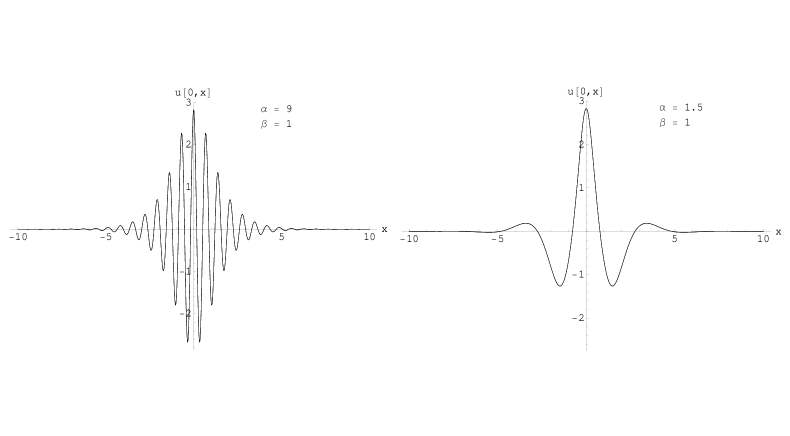
Figure 1. Left: mKdV breather (1.8) with $\alpha=9,\beta=1$ at $t=0$.  Right: mKdV breather (1.8) with $\alpha=1.5,\beta=1$ at $t=0$.

Note that from the invariance under space and time translations, given any $t_{0},x_{0}\in\mathbb{R}$, the function $B_{\alpha,\beta}(t-t_{0},x-x_{0})$ is also a breather solution. This fact allows to define a four-parameter family of solutions

$$B_{\alpha,\beta}(t,x;x_{1},x_{2}):=B_{\alpha,\beta}(t-t_{0},x-x_{0})=2\sqrt{2}\partial_{x}\Big{[}\arctan\Big{(}\frac{\beta}{\alpha}\frac{\sin(\alpha y_{1})}{\cosh(\beta y_{2})}\Big{)}\Big{]},$$ (1.11)

with $y_{1}:=x+\delta t+x_{1}$, $y_{2}:=x+\gamma t+x_{2}$,

$$t_{0}:=\frac{x_{1}-x_{2}}{2(\alpha^{2}+\beta^{2})},\quad\hbox{ and }\quad x_{0}:=\frac{\delta x_{2}-\gamma x_{1}}{2(\alpha^{2}+\beta^{2})}.$$ (1.12)

Note that from this formula one has, for any $k\in\mathbb{Z}$,

$$B_{\alpha,\beta}(t,x;x_{1}+\frac{k\pi}{\alpha},x_{2})=(-1)^{k}B_{\alpha,\beta}(t,x;x_{1},x_{2}),$$ (1.13)

which are also solutions of (1.1). These identities reveal the periodic character of the first translation parameter.

In the same way, from (1.10) one can define a three-parameter family of double pole solutions $B_{0,\beta}(t;x_{1},x_{2})$, with $x_{1},x_{2}\in\mathbb{R}$. a

Figure 2. Evolution of the mKdV breather (1.8) with $\alpha=7,\beta=1$ at instants $t=-0.09$, $t=0$, and $t=0.13$. Note that with the selected values of $\alpha,\beta$, the velocity is given by $\gamma=3\alpha^{2}-\beta^{2}=146>0$ and then the breather moves to the left.

a

Let us come back to breather solutions. We claim that they can be formally associated to the well known mKdV 2-solitons. Indeed, they have a four-parameter family of symmetries: two scaling and two translations invariances (note that the equation that we consider is just one dimensional in space). However, unlike 2-soliton solutions, breathers have to be considered as fully bounded states, since they do not decouple into simple solitons as time evolves. Another intriguing fact is that, as far as we know, breathers are only present in some very particular integrable models, such as mKdV, NLS and sine Gordon equations, among others.

Let us recall now some relevant physical and mathematical literature. From the physical point of view, breather solutions are relevant to localization-type phenomena in optics, condensed matter physics and biophysics [8]. In a geometrical setting, breathers also appear in the evolution of closed planar curves playing the role of smooth localized deformations traveling along the closed curve [3]. Moreover, it is interesting to stress that breather solutions have also been considered by Kenig, Ponce and Vega in their proof of the non-uniform continuity of the mKdV flow in the Sobolev spaces $H^{s}$, $s<\frac{1}{4}$ [20]. On the other hand, they should be essential to completely understand the associated soliton-resolution conjecture for the mKdV equation, according to the analysis developed by Schuur in [34]. An essential problem in that direction is to show whether or not breather solutions may appear from general initial data, and for this reason to study their stability is the fundamental question. Numerical computations (see Gorria-Alejo-Vega [5]) show that breathers are numerically stable. However, the simple question of a rigorous proof of orbital stability has become a long standing open problem.

In this paper, we give a first, positive answer to the question of breathers stability. Our main result is the following

Theorem 1.2.

mKdV breathers are orbitally stable in their natural $H^{2}$-topology.

A more detailed version of this result is given in Theorem 6.1. As we will see from the proofs, the space $H^{2}$ is required by a regularity argument and by the very important fact that breathers are bound states, which means that there is no mass decoupling as time evolves. However, our argument is general and can be applied to several equations with breather solutions, and moreover, it introduces several new ideas in order to attack the stability problem in the energy space. In addition, our proof corroborates, at the rigorous level, some deep connections between breathers and the 2-solitons of mKdV.

Let us explain the main steps of the proof. First, we prove that breathers satisfy a fourth-order, nonlinear ODE (equation (3.6)). The proof of this identity is involved, and requires the explicit form of the breather, and several new identities related to the soliton structure of the breather. It seems that this equation cannot be obtained from the original arguments by Lax [22], since the dynamics do not decouple in time. Our second and more important ingredient is the introduction of a new Lyapunov functional (see (5.2)), well-defined in the $H^{2}$ topology, and for which breathers are surprisingly not only extremal points, but also local minimizers, up to symmetries. This functional also allows to control the perturbative terms and the instability directions that appear during of the dynamics, the latter as consequences of the symmetries described by (1.8). From the proofs, we will see that breathers have essentially three directions of instability, two associated to translation invariances, and a third one consequence of the particular first scaling parameter $\beta$. In order to prove that there is just one negative eigenvalue, we make use of a direct generalization of the theory developed by L. Greenberg [15], which deals with fourth order eigenvalue problems. We then modulate in time in order to remove the spatial instabilities. This is an absolutely necessary condition in order to obtain an orbital stability property. However, we do not modulate the scaling instabilities. Instead, we control the dynamics first replacing the corresponding negative mode by a more tractable direction, the breather itself, and using the mass conservation law. This technique was first introduced by Weinstein in [37]. A very surprising fact is that the so-called second scaling parameter, associated to oscillations, is actually a positive direction when enough regularity is on hand, and even if it has an $L^{2}$-critical character.

Our functional is reminiscent of that appearing in the foundational paper by Lax [22], concerning the 2-soliton solution of the KdV equation,

$$u_{t}+(u_{xx}+u^{2})_{x}=0,$$

and generalized to the KdV $N$-soliton states by Maddock-Sachs [23]. This idea has been successfully applied to several 2-soliton problems, for which the dynamics decouples into well-separated solitons as time evolves, see e.g. Holmer-Perelman-Zworski [17], Kapitula [18], and Lopes-Neves [30], for the Benjamin-Ono equation. However, there was no evidence that this technique could be generalized to the case of even more complex solutions, such as breathers. Compared with those results, our proofs are more involved, and computations are sometimes a nightmare. We have preferred to split the proof of the main theorem into several simple steps.

We believe that our result can be improved to reach the $H^{1}$ level of regularity, but with a harder proof. It seems clear that a better understanding of the $H^{1}$ dynamics requires a detailed study of modulations on the scaling parameters. In particular, the Martel-Merle-Tsai technique [28] seems to fail in this case due to the absence of a clearly decoupled mass dynamics. One can also consider a suitable asymptotic stability property, in the spirit of [24]. However, note that the Martel-Merle [24, 25, 27] results are difficult to generalize to the current case of study since breathers may have negative velocity, and therefore they can interact with the linear part of the dynamics. We conjecture that breathers are asymptotically stable in the case of positive velocities.

Remark 1.1.

The methods employed in the proof of Theorem 1.2 seem do not apply in the limit $\alpha\to 0$, which is expected to be unstable, according to the numerical computations performed by Gorria-Alejo-Vega [5].

Remark 1.2.

The natural complement of our study is to consider the sine Gordon equation

$$u_{tt}-u_{xx}+\sin u=0,\quad u(t,x)\in\mathbb{R}.$$

Since this integrable equation has also breather solutions (see e.g. Lamb [21]), we expect similar results, but with more involved proofs at the level of the linearized problem (we deal with matrix operators). Indeed, following the present proof, we can guess that sine-Gordon breathers are $H^{2}\times H^{1}$ stable provided Lemma 4.3 and Proposition 4.8 hold for the associated spectral elements. Additionally, the focusing Gardner equation

$$u_{t}+(u_{xx}+u^{2}+\mu u^{3})_{x}=0,\quad\mu>0,$$

is the natural generalization of (1.1). In particular, it has a family of breathers indexed by the additional parameter $\mu$ (see [33, 4]). We expect to consider some of these problems in a forthcoming publication (see [6]).

In a more qualitative aspect, we think that our results are in some sense a surprise, because any nontrivial perturbation of an integrable equation with breathers solutions should destroy the existence property. Several results in that direction can be found e.g. in [10, 13, 35] and references therein (for the sine Gordon case). Those results and the present paper suggest that stability is deeply related to the integrability of the equation, unlike the standard gKdV $N$-soliton solution [28].

Finally, let us explain the organization of this paper. In Section 2 we study generalized Weinstein conditions satisfied by breather solutions. In Section 3 we prove that any breather profile satisfies a fourth order, nonlinear ODE. Section 4 is devoted to the study of a linear operator associated to the breather solution. In Section 5 we introduce new Lyapunov functional which controls the dynamics. Finally, in Section 6 we prove a detailed version of Theorem 1.2.

Acknowdlegments. We would like to thank Yvan Martel, Frank Merle, Carlos Kenig and Luis Vega for many useful comments on a first version of this paper.

2. Stability tests

The purpose of this section is to obtain generalized Weinstein conditions for any breather $B$. Indeed, for the case of the mKdV soliton (1.4), the mass (1.2) and the energy (1.3) are given by the quantities

$$M[Q_{c}]=\frac{1}{2}c^{1/2}\int_{\mathbb{R}}Q^{2}=2c^{1/2},$$ (2.1)

$$E[Q_{c}]=c^{3/2}E[Q]=-\frac{1}{3}c^{3/2}M[Q]=-\frac{2}{3}c^{3/2}<0.$$ (2.2)

These two identities show the explicit dependence of the mass and the energy on the soliton scaling parameter. In particular, the Weinstein condition [38] reads, for $c>0$,

$$\partial_{c}M[Q_{c}]=c^{-1/2}>0.$$ (2.3)

This condition ensures the nonlinear stability of the soliton. We consider now the case of mKdV breathers. Surprisingly enough, the mass of a mKdV breather only depends on the first scaling parameter $\beta$. In other words, it is independent of $\alpha$.

Lemma 2.1.

Let $B=B_{\alpha,\beta}$ be any mKdV breather, for $\alpha,\beta>0$. Then

$$M[B](t)=2\beta M[Q]=4\beta.$$ (2.4)

Proof.

We start by writing the breather solution in a more tractable way. From the conservation of mass and invariance under spatial and time translations, we can assume $x_{1}=x_{2}=t=0$ in (1.11). We have then

$$B^{2}(0,x)=8\beta^{2}\operatorname{sech}^{2}(\beta x)\Big{[}\frac{\cos(\alpha x)-(\beta/\alpha)\sin(\alpha x)\tanh(\beta x)}{1+(\beta/\alpha)^{2}\sin^{2}(\alpha x)\operatorname{sech}^{2}(\beta x)}\Big{]}^{2}.$$

Expanding the square in the numerator, we get after some simplifications

$$B^{2}(0,x)=8\alpha^{2}\beta^{2}\times$$

$$\times\Big{[}\frac{\alpha^{2}\cosh^{2}(\beta x)\cos^{2}(\alpha x)+\beta^{2}\sin^{2}(\alpha x)\sinh^{2}(\beta x)-2\alpha\beta\sin(\alpha x)\cos(\alpha x)\sinh(\beta x)\cosh(\beta x)}{(\alpha^{2}\cosh^{2}(\beta x)+\beta^{2}\sin^{2}(\alpha x))^{2}}\Big{]}.$$

Now the purpose is to use double angle formulas to avoid the squares. More precisely, it is well known that

$$\cos^{2}(\alpha x)=\frac{1}{2}(1+\cos(2\alpha x)),\quad\sin^{2}(\alpha x)=\frac{1}{2}(1-\cos(2\alpha x)),$$ (2.5)

and

$$\cosh^{2}(\beta x)=\frac{1}{2}(1+\cosh(2\beta x)),\quad\sinh^{2}(\beta x)=\frac{1}{2}(\cosh(2\beta x)-1).$$ (2.6)

We replace these identities in the previous expression above. We obtain

$$B^{2}(0,x)=\frac{8\alpha^{2}\beta^{2}h_{\alpha,\beta}(x)}{(\alpha^{2}+\beta^{2}+\alpha^{2}\cosh(2\beta x)-\beta^{2}\cos(2\alpha x))^{2}},$$

with

$$h_{\alpha,\beta}(x) :=\alpha^{2}-\beta^{2}+(\alpha^{2}+\beta^{2})(\cos(2\alpha x)+\cosh(2\beta x))$$

$$\qquad+(\alpha^{2}-\beta^{2})\cos(2\alpha x)\cosh(2\beta x)-2\alpha\beta\sin(2\alpha x)\sinh(2\beta x).$$ (2.7)

In what follows, let

$$f_{\alpha,\beta}(x):=\alpha^{2}+\beta^{2}+\alpha\beta\sin(2\alpha x)-\beta^{2}\cos(2\alpha x)+\alpha^{2}(\sinh(2\beta x)+\cosh(2\beta x)),$$

and

$$g_{\alpha,\beta}(x):=\alpha^{2}+\beta^{2}+\alpha^{2}\cosh(2\beta x)-\beta^{2}\cos(2\alpha x).$$

It is clear that

$$f^{\prime}_{\alpha,\beta}(x)=2\alpha\beta[\alpha\cos(2\alpha x)+\beta\sin(2\alpha x)+\alpha\cosh(2\beta x)+\alpha\sinh(2\beta x)],$$

and

$$g^{\prime}_{\alpha,\beta}(x)=2\alpha\beta[\beta\sin(2\alpha x)+\alpha\sinh(2\beta x)].$$

Therefore, after a lengthy but direct computation,

$$f^{\prime}_{\alpha,\beta}(x)g_{\alpha,\beta}(x)-f_{\alpha,\beta}(x)g^{\prime}_{\alpha,\beta}(x)=2\alpha^{2}\beta h_{\alpha,\beta}(x),$$

and then

$$B^{2}(0,x)=4\beta\frac{f^{\prime}_{\alpha,\beta}(x)g_{\alpha,\beta}(x)-f_{\alpha,\beta}(x)g^{\prime}_{\alpha,\beta}(x)}{g_{\alpha,\beta}^{2}(x)}=4\beta\Big{(}\frac{f_{\alpha,\beta}}{g_{\alpha,\beta}}\Big{)}^{\prime}.$$

In conclusion, we have proved that

$$\frac{1}{2}\int_{-\infty}^{x}B^{2}(0,s)ds=\frac{2\beta[\alpha^{2}+\beta^{2}+\alpha\beta\sin(2\alpha x)-\beta^{2}\cos(2\alpha x)+\alpha^{2}(\sinh(2\beta x)+\cosh(2\beta x))]}{\alpha^{2}+\beta^{2}+\alpha^{2}\cosh(2\beta x)-\beta^{2}\cos(2\alpha x)}.$$

Taking limit as $x\to+\infty$, we get the desired conclusion. ∎

Remark 2.1.

Note that the last integral above does not change if we consider a general breather, of the form (1.11). Indeed, our proof does not require the time independence of the solution. Then we get

$$\mathcal{M}_{\alpha,\beta}(t,x) :=\frac{1}{2}\int_{-\infty}^{x}B_{\alpha,\beta}^{2}(t,s;x_{1},x_{2})ds$$

$$\leavevmode\nobreak\ =\frac{2\beta[\alpha^{2}+\beta^{2}+\alpha\beta\sin(2\alpha y_{1})-\beta^{2}\cos(2\alpha y_{1})+\alpha^{2}(\sinh(2\beta y_{2})+\cosh(2\beta y_{2}))]}{\alpha^{2}+\beta^{2}+\alpha^{2}\cosh(2\beta y_{2})-\beta^{2}\cos(2\alpha y_{1})},$$ (2.8)

with $y_{1}$ and $y_{2}$ defined in (1.11). This last expression will be useful in Lemma 2.3.

A direct consequence of the results above are the following generalized Weinstein conditions:

Corollary 2.2.

Let $B=B_{\alpha,\beta}$ be any mKdV breather of the form (1.11). Given $t\in\mathbb{R}$ fixed, let

$$\Lambda_{\alpha}B:=\partial_{\alpha}B,\quad\hbox{ and }\quad\Lambda_{\beta}B:=\partial_{\beta}B.$$ (2.9)

Then both functions $\Lambda_{\alpha}B$ and $\Lambda_{\beta}B$ are in the Schwartz class for the spatial variable, and satisfy the identities

$$\partial_{\alpha}M[B]=\int_{\mathbb{R}}B\Lambda_{\alpha}B=0,$$ (2.10)

and

$$\partial_{\beta}M[B]=\int_{\mathbb{R}}B\Lambda_{\beta}B=4>0,$$ (2.11)

independently of time.

Proof.

By simple inspection, one can see that, given $t$ fixed, $\Lambda_{\alpha}B_{\alpha,\beta}$ and $\Lambda_{\beta}B_{\alpha,\beta}$ are well-defined Schwartz functions. The proof of (2.10) and (2.11) is consequence of (2.4), and the definition of mass (1.2). ∎

Remark 2.2.

Comparing (2.10) and (2.11) with the Weinstein condition (2.3), we may think that the second scaling parameter $\alpha$ is $L^{2}$-critical. On the opposite side, the first scaling $\beta$ can be seen as a stable parameter.

Lemma 2.3.

Let $B=B_{\alpha,\beta}$ be any breather of the form (1.11), with $\alpha,\beta>0$. Then we have

1. $B=\tilde{B}_{x}$, with $\tilde{B}=\tilde{B}_{\alpha,\beta}$ given by the smooth $L^{\infty}$-function

   $$\tilde{B}(t,x):=2\sqrt{2}\arctan\Big{(}\frac{\beta}{\alpha}\frac{\sin(\alpha y_{1})}{\cosh(\beta y_{2})}\Big{)}.$$ (2.12)

2. For any fixed $t\in\mathbb{R}$, we have $\tilde{B}_{t}$ well-defined in the Schwartz class, satisfiying

   $$B_{xx}+\tilde{B}_{t}+B^{3}=0.$$ (2.13)

3. Finally, let $\mathcal{M}_{\alpha,\beta}$ be defined by (2.1). Then

   $$B_{x}^{2}+\frac{1}{2}B^{4}+2B\tilde{B}_{t}-2(\mathcal{M}_{\alpha,\beta})_{t}=0.$$ (2.14)

Proof.

The first item above is a direct consequence of the definition of $B_{\alpha,\beta}$ in (1.11). On the other hand, (2.13) is a consequence of (2.12) and integration in space (from $-\infty$ to $x$) of (1.1). Finally, to obtain (2.14) we multiply (2.13) by $B_{x}$ and integrate in space. ∎

Remark 2.3.

The reader may compare (2.13)-(2.14) with the well known identities for the soliton solution of mKdV:

$$Q_{c}^{\prime\prime}-cQ_{c}+Q_{c}^{3}=0,\qquad Q_{c}^{\prime 2}-cQ_{c}^{2}+\frac{1}{2}Q_{c}^{4}=0.$$

We compute now the energy of a breather solution.

Lemma 2.4.

Let $B=B_{\alpha,\beta}$ be any mKdV breather, for $\alpha,\beta>0$. Then

$$E[B]=2\beta(3\alpha^{2}-\beta^{2})|E[Q]|=2\beta\gamma|E[Q]|.$$ (2.15)

Let us remark that the sign of the energy is dictated by the sign of the velocity $\gamma$.

Proof.

First of all, let us prove the following reduction

$$E[B](t)=\frac{1}{3}\int_{\mathbb{R}}(\mathcal{M}_{\alpha,\beta})_{t}(t,x)dx.$$ (2.16)

Indeed, we multiply (2.13) by $B_{\alpha,\beta}$ and integrate in space: we get

$$\int_{\mathbb{R}}B_{x}^{2}=\int_{\mathbb{R}}B\tilde{B}_{t}+\int_{\mathbb{R}}B^{4}.$$

On the other hand, integrating (2.14),

$$\int_{\mathbb{R}}B_{x}^{2}+\frac{1}{2}\int_{\mathbb{R}}B^{4}+2\int_{\mathbb{R}}B\tilde{B}_{t}-2\int_{\mathbb{R}}(\mathcal{M}_{\alpha,\beta})_{t}=0.$$

From these two identities, we get

$$\int_{\mathbb{R}}B^{4}=\frac{4}{3}\int_{\mathbb{R}}(\mathcal{M}_{\alpha,\beta})_{t}-2\int_{\mathbb{R}}B\tilde{B}_{t},$$

and therefore

$$\int_{\mathbb{R}}B_{x}^{2}=\frac{4}{3}\int_{\mathbb{R}}(\mathcal{M}_{\alpha,\beta})_{t}-\int_{\mathbb{R}}B\tilde{B}_{t}.$$

Finally, replacing the last two identities in (1.3), we get (2.16), as desired.

Now we prove (2.15). From (2.1) and similar to the proof of Lemma 2.1, we have

$$(\mathcal{M}_{\alpha,\beta})_{t}=2\beta\frac{(f_{\alpha,\beta})_{t}g_{\alpha,\beta}-f_{\alpha,\beta}(g_{\alpha,\beta})_{t}}{g_{\alpha,\beta}^{2}},$$

where, with a slight abuse of notation, $f_{\alpha,\beta}$ and $g_{\alpha,\beta}$ are given now by

$$f_{\alpha,\beta}=\alpha^{2}+\beta^{2}+\alpha\beta\sin(2\alpha y_{1})-\beta^{2}\cos(2\alpha y_{1})+\alpha^{2}(\sinh(2\beta y_{2})+\cosh(2\beta y_{2})),$$

and

$$g_{\alpha,\beta}=\alpha^{2}+\beta^{2}+\alpha^{2}\cosh(2\beta y_{2})-\beta^{2}\cos(2\alpha y_{1}).$$ (2.17)

It is clear that

$$(f_{\alpha,\beta})_{t}=2\alpha\beta[\alpha\delta\cos(2\alpha y_{1})+\beta\delta\sin(2\alpha y_{1})+\alpha\gamma\cosh(2\beta y_{2})+\alpha\gamma\sinh(2\beta y_{2})],$$

and

$$(g_{\alpha,\beta})_{t}=2\alpha\beta[\beta\delta\sin(2\alpha y_{1})+\alpha\gamma\sinh(2\beta y_{2})].$$

Therefore

$$(f_{\alpha,\beta})_{t}g_{\alpha,\beta}-f_{\alpha,\beta}(g_{\alpha,\beta})_{t}=2\alpha^{2}\beta\tilde{h}_{\alpha,\beta},$$

and

$$\tilde{h}_{\alpha,\beta} :=\gamma\alpha^{2}-\delta\beta^{2}+(\alpha^{2}+\beta^{2})(\delta\cos(2\alpha y_{1})+\gamma\cosh(2\beta y_{2}))$$

$$\qquad+(\delta\alpha^{2}-\gamma\beta^{2})\cos(2\alpha y_{1})\cosh(2\beta y_{2})-\alpha\beta(\delta+\gamma)\sin(2\alpha y_{1})\sinh(2\beta y_{2}).$$ (2.18)

In conclusion,

$$\frac{1}{3}(\mathcal{M}_{\alpha,\beta})_{t}=\frac{4\alpha^{2}\beta^{2}\tilde{h}_{\alpha,\beta}}{3(\alpha^{2}+\beta^{2}+\alpha^{2}\cosh(2\beta y_{2})-\beta^{2}\cos(2\alpha y_{1}))^{2}}.$$ (2.19)

Now we split $\tilde{h}_{\alpha,\beta}$ into two pieces, according to the parameter $\gamma$. From the definition of $\gamma$, $\delta$ and $h_{\alpha,\beta}$, we have

$$\tilde{h}_{\alpha,\beta}=\gamma h_{\alpha,\beta}+2(\alpha^{2}+\beta^{2})\hat{h}_{\alpha,\beta},$$

where

$$\hat{h}_{\alpha,\beta}:=\beta^{2}-(\alpha^{2}+\beta^{2})\cos(2\alpha y_{1})-\alpha^{2}\cos(2\alpha y_{1})\cosh(2\beta y_{2})+\alpha\beta\sin(2\alpha y_{1})\sinh(2\beta y_{2}).$$

Note that from Lemma 2.1, more precisely (2.1),

$$\int_{\mathbb{R}}\frac{4\alpha^{2}\beta^{2}\gamma h_{\alpha,\beta}}{3(\alpha^{2}+\beta^{2}+\alpha^{2}\cosh(2\beta y_{2})-\beta^{2}\cos(2\alpha y_{1}))^{2}}=\frac{4}{3}\beta\gamma=2\beta\gamma|E[Q]|,$$

then, in order to conclude, from (2.19) and (2.16) we reduce to prove that

$$\int_{\mathbb{R}}\frac{\hat{h}_{\alpha,\beta}}{(\alpha^{2}+\beta^{2}+\alpha^{2}\cosh(2\beta y_{2})-\beta^{2}\cos(2\alpha y_{1}))^{2}}=0.$$ (2.20)

We prove this identity, noting that $(\frac{1}{2\alpha}\sin(2\alpha y_{1}))_{x}=\cos(2\alpha y_{1})$, and from (2.17),

$$g_{\alpha,\beta}(\frac{1}{2\alpha}\sin(2\alpha y_{1}))_{x}-\frac{1}{2\alpha}\sin(2\alpha y_{1})(g_{\alpha,\beta})_{x}=$$

$$\quad=\cos(2\alpha y_{1})[\alpha^{2}+\beta^{2}+\alpha^{2}\cosh(2\beta y_{2})-\beta^{2}\cos(2\alpha y_{1})]-\beta\sin(2\alpha y_{1})[\beta\sin(2\alpha y_{1})+\alpha\sinh(2\beta y_{2})]$$

$$\quad=-\beta^{2}(\cos^{2}(2\alpha y_{1})+\sin^{2}(2\alpha y_{1}))+(\alpha^{2}+\beta^{2})\cos(2\alpha y_{1})+\alpha^{2}\cos(2\alpha y_{1})\cosh(2\beta y_{2})$$

$$\qquad\qquad-\alpha\beta\sin(2\alpha y_{1})\sinh(2\beta y_{2})$$

$$\quad=-\hat{h}_{\alpha,\beta}.$$

Therefore,

$$\hbox{ l.h.s. of (\ref{int0})}=\lim_{x\to+\infty}\frac{-\sin(2\alpha y_{1})}{2\alpha(\alpha^{2}+\beta^{2}+\alpha^{2}\cosh(2\beta y_{2})-\beta^{2}\cos(2\alpha y_{1}))}=0.$$

∎

Remark 2.4.

Note that we could follow the approach by Lax [22, pp. 479–481] to obtain reduced expressions for the mass and energy of a breather solution. However, the resulting terms are actually harder to manage than our direct approach.

Corollary 2.5.

Let $B=B_{\alpha,\beta}$ be any mKdV breather. Then

$$\partial_{\alpha}E[B]=12\alpha\beta|E[Q]|>0,\quad\partial_{\beta}E[B]=6(\alpha^{2}-\beta^{2})|E[Q]|.$$ (2.21)

3. Nonlinear stationary equations

The objective of this section is to prove that any breather profile satisfies a suitable stationary, elliptic equation.

Lemma 3.1.

Let $B=B_{\alpha,\beta}$ be any mKdV breather. Then, for all $t\in\mathbb{R}$,

$$B_{xt}+2(\mathcal{M}_{\alpha,\beta})_{t}B=2(\beta^{2}-\alpha^{2})\tilde{B}_{t}+(\alpha^{2}+\beta^{2})^{2}B.$$ (3.1)

Proof.

We make use of the explicit expression of the breather. An equivalent for the quantity $(\mathcal{M}_{\alpha,\beta})_{t}$ has been already computed in Lemma 2.4, see (2.19). On the other hand, from (2.12) and (1.11), and using double angle formulas in the denominator, we have,

$$\tilde{B}_{t}=4\sqrt{2}\alpha\beta\Big{[}\frac{\alpha\delta\cos(\alpha y_{1})\cosh(\beta y_{2})-\beta\gamma\sin(\alpha y_{1})\sinh(\beta y_{2})}{\alpha^{2}+\beta^{2}+\alpha^{2}\cosh(2\beta y_{2})-\beta^{2}\cos(2\alpha y_{1})}\Big{]}.$$ (3.2)

From (1.8) we have

$$B =2\sqrt{2}\alpha\beta\Big{[}\frac{\alpha\cos(\alpha y_{1})\cosh(\beta y_{2})-\beta\sin(\alpha y_{1})\sinh(\beta y_{2})}{\alpha^{2}\cosh^{2}(\beta y_{2})+\beta^{2}\sin^{2}(\alpha y_{1})}\Big{]}$$ (3.3)

$$=4\sqrt{2}\alpha\beta\Big{[}\frac{\alpha\cos(\alpha y_{1})\cosh(\beta y_{2})-\beta\sin(\alpha y_{1})\sinh(\beta y_{2})}{\alpha^{2}+\beta^{2}+\alpha^{2}\cosh(2\beta y_{2})-\beta^{2}\cos(2\alpha y_{1})}\Big{]}.$$ (3.4)

Therefore, from (3.3) and (2.19),

$$(\mathcal{M}_{\alpha,\beta})_{t}B=\frac{16\sqrt{2}\alpha^{3}\beta^{3}\tilde{\theta}(t,x)}{(\alpha^{2}+\beta^{2}+\alpha^{2}\cosh(2\beta y_{2})-\beta^{2}\cos(2\alpha y_{1}))^{3}}$$

where, with the definition of $\tilde{h}$ in (2.18),

$$\tilde{\theta}(t,x):=\tilde{h}_{\alpha,\beta}(\alpha\cos(\alpha y_{1})\cosh(\beta y_{2})-\beta\sin(\alpha y_{1})\sinh(\beta y_{2})).$$

Let us compute $B_{xt}$. First we have from (3.3),

$$B_{x}=\frac{4\sqrt{2}\alpha\beta h_{1}(t,x)}{(\alpha^{2}+\beta^{2}+\alpha^{2}\cosh(2\beta y_{2})-\beta^{2}\cos(2\alpha y_{1}))^{2}},$$

where

$$h_{1}(t,x) :=-(\alpha^{2}+\beta^{2})\cosh(\beta y_{2})\sin(\alpha y_{1})[\alpha^{2}+\beta^{2}+\alpha^{2}\cosh(2\beta y_{2})-\beta^{2}\cos(2\alpha y_{1})]$$

$$-2\alpha\beta[\alpha\cos(\alpha y_{1})\cosh(\beta y_{2})-\beta\sin(\alpha y_{1})\sinh(\beta y_{2})][\beta\sin(2\alpha y_{1})+\alpha\sinh(2\beta y_{2})].$$

Then,

$$B_{xt}=\frac{4\sqrt{2}\alpha\beta h_{2}}{(\alpha^{2}+\beta^{2}+\alpha^{2}\cosh(2\beta y_{2})-\beta^{2}\cos(2\alpha y_{1}))^{3}},$$

where, using $g_{\alpha,\beta}$ previously defined in (2.17),

$$h_{2}(t,x):=-4\alpha\beta\big{[}\beta\delta\sin(2\alpha y_{1})+\alpha\gamma\sinh(2\beta y_{2})\big{]}h_{21}+g_{\alpha,\beta}h_{22},$$

and

$$h_{21}(t,x) :=-(\alpha^{2}+\beta^{2})\cosh(\beta y_{2})\sin(\alpha y_{1})g_{\alpha,\beta}$$

$$-2\alpha\beta(\alpha\cos(\alpha y_{1})\cosh(\beta y_{2})-\beta\sin(\alpha y_{1})\sinh(\beta y_{2}))(\beta\sin(2\alpha y_{1})+\alpha\sinh(2\beta y_{2})),$$

$$h_{22}(t,x):= \ g_{\alpha,\beta}\times\Big{[}\big{(}-\alpha\delta(\alpha^{2}+\beta^{2})\cos(\alpha y_{1})\cosh(\beta y_{2})-\beta\gamma(\alpha^{2}+\beta^{2})\sin(\alpha y_{1})\sinh(\beta y_{2})\big{)}g_{\alpha,\beta}$$

$$-2\alpha\beta(\alpha^{2}+\beta^{2})\sin(\alpha y_{1})\cosh(\beta y_{2})\big{(}\alpha\gamma\sinh(2\beta y_{2})+\delta\beta\sin(2\alpha y_{1})\big{)}$$

$$-2\alpha\beta\big{(}-\alpha^{2}\delta\sin(\alpha y_{1})\cosh(\beta y_{2})+\alpha\beta\gamma\cos(\alpha y_{1})\sinh(\beta y_{2})$$

$$-\beta\alpha\delta\cos(\alpha y_{1})\sinh(\beta y_{2})-\beta^{2}\gamma\sin(\alpha y_{1})\cosh(\beta y_{2})\big{)}\times\big{(}\alpha\sinh(2\beta y_{2})+\beta\sin(2\alpha y_{1})\big{)}$$

$$-4\alpha^{2}\beta^{2}\big{(}\alpha\cos(\alpha y_{1})\cosh(\beta y_{2})-\beta\sin(\alpha y_{1})\sinh(\beta y_{2})\big{)}\times\big{(}\gamma\cosh(2\beta y_{2})+\delta\cos(2\alpha y_{1})\big{)}\Big{]}.$$

Then,

$$B_{xt}+2(\mathcal{M}_{\alpha,\beta})_{t}B=\frac{4\sqrt{2}\alpha\beta\big{[}h_{2}+8\alpha^{2}\beta^{2}\tilde{\theta}\big{]}}{(\alpha^{2}+\beta^{2}+\alpha^{2}\cosh(2\beta y_{2})-\beta^{2}\cos(2\alpha y_{1}))^{3}},$$ (3.5)

and recalling that

$$g_{\alpha,\beta}^{2}=(\alpha^{2}+\beta^{2}+\alpha^{2}\cosh(2\beta y_{2})-\beta^{2}\cos(2\alpha y_{1}))^{2}$$

$$=(\alpha^{2}+\beta^{2})^{2}+(\alpha^{4}\cosh(2\beta y_{2})^{2}+\beta^{4}\cos(2\alpha y_{1})^{2}-2\alpha^{2}\beta^{2}\cosh(2\beta y_{2})\cos(2\alpha y_{1}))$$

$$-2(\alpha^{2}+\beta^{2})(\alpha^{2}\cosh(2\beta y_{2})-\beta^{2}\cos(2\alpha y_{1})),$$

collecting terms in (3.5) and taking into account (3.4) and (3.2), after some calculations we have

$$\hbox{r.h.s. of }\eqref{lhs31} =\frac{4\sqrt{2}\alpha\beta}{(\alpha^{2}+\beta^{2}+\alpha^{2}\cosh(2\beta y_{2})-\beta^{2}\cos(2\alpha y_{1}))^{3}}\times$$

$$\Big{\{}g_{\alpha,\beta}^{2}\times\Big{[}2(\beta^{2}-\alpha^{2})\big{(}\delta\alpha\cos(\alpha y_{1})\cosh(\beta y_{2})-\gamma\beta\sin(\alpha y_{1})\sinh(\beta y_{2})\big{)}$$

$$+(\alpha^{2}+\beta^{2})^{2}\big{(}\alpha\cos(\alpha y_{1})\cosh(\beta y_{2})-\beta\sin(\alpha y_{1})\sinh(\beta y_{2})\big{)}\Big{]}\Big{\}}$$

$$=2(\beta^{2}-\alpha^{2})(\tilde{B}_{\alpha,\beta})_{t}+(\alpha^{2}+\beta^{2})^{2}B_{\alpha,\beta}.$$

∎

In what follows, and for the sake of simplicity, we use the notation $B=B_{\alpha,\beta}$ and $\mathcal{M}_{t}=(\mathcal{M}_{\alpha,\beta})_{t}$, if no confusion is present.

Proposition 3.2.

Let $B=B_{\alpha,\beta}$ be any mKdV breather. Then, for any fixed $t\in\mathbb{R}$, $B$ satisfies the nonlinear stationary equation

$$G[B]:=B_{(4x)}-2(\beta^{2}-\alpha^{2})(B_{xx}+B^{3})+(\alpha^{2}+\beta^{2})^{2}B+5BB_{x}^{2}+5B^{2}B_{xx}+\frac{3}{2}B^{5}=0.$$ (3.6)

Remark 3.1.

This identity can be seen as the nonlinear, stationary equation satisfied by the breather profile, and therefore it is independent of time and translation parameters $x_{1},x_{2}\in\mathbb{R}$. One can compare with the soliton profile $Q_{c}(x-ct-x_{0})$, which satisfies the standard elliptic equation (1.5), obtained as the first variation of the $H^{1}$ Weinstein functional (1.6).

Proof of Proposition 3.2.

From (2.13) and (2.14), one has

$$\hbox{l.h.s. of }(\ref{EcB}) =-(B_{t}+B^{3})_{xx}+2(\beta^{2}-\alpha^{2})\tilde{B}_{t}+(\alpha^{2}+\beta^{2})^{2}B+5BB_{x}^{2}+5B^{2}B_{xx}+\frac{3}{2}B^{5}$$

$$=-B_{tx}-BB_{x}^{2}+2B^{2}B_{xx}+2(\beta^{2}-\alpha^{2})\tilde{B}_{t}+(\alpha^{2}+\beta^{2})^{2}B+\frac{3}{2}B^{5}$$

$$=-B_{tx}+B\Big{[}\frac{1}{2}B^{4}+2B\tilde{B}_{t}-2\mathcal{M}_{t}\Big{]}-2B^{2}(\tilde{B}_{t}+B^{3})+\frac{3}{2}B^{5}$$

$$\qquad+2(\beta^{2}-\alpha^{2})\tilde{B}_{t}+(\alpha^{2}+\beta^{2})^{2}B$$

$$=-[B_{tx}+2\mathcal{M}_{t}B]+2(\beta^{2}-\alpha^{2})\tilde{B}_{t}+(\alpha^{2}+\beta^{2})^{2}B\ =0.$$

In the last line we have used (3.1). ∎

Corollary 3.3.

Let $B^{0}_{\alpha,\beta}=B^{0}_{\alpha,\beta}(t,x;0,0)$ be any mKdV breather as in (1.8), and $x_{1}(t),x_{2}(t)\in\mathbb{R}$ two continuous functions, defined for all $t$ in a given interval. Consider the modified breather

$$B_{\alpha,\beta}(t,x):=B^{0}_{\alpha,\beta}(t,x;x_{1}(t),x_{2}(t)),\qquad(\hbox{cf. \eqref{BB}}).$$

Then $B_{\alpha,\beta}$ satisfies (3.6), for all $t$ in the considered interval.

Proof.

A direct consequence of the invariance of the equation (3.6) under spatial translations. Note that (3.6) is satisfied even if $B_{\alpha,\beta}$ is not an exact solution of (1.1). ∎

4. Spectral analysis

Let $z=z(x)$ be a function to be specified in the following lines. Let $B=B_{\alpha,\beta}$ be any breather solution, with shift parameters $x_{1},x_{2}$. Let us introduce the following fourth order linear operator:

$$\mathcal{L}[z](x;t) :=z_{(4x)}(x)-2(\beta^{2}-\alpha^{2})z_{xx}(x)+(\alpha^{2}+\beta^{2})^{2}z(x)+5B^{2}z_{xx}(x)+10BB_{x}z_{x}(x)$$

$$\qquad+\ \big{[}5B_{x}^{2}+10BB_{xx}+\frac{15}{2}B^{4}-6(\beta^{2}-\alpha^{2})B^{2}\big{]}z(x).$$ (4.1)

In this section we describe the spectrum of this operator. More precisely, our main purpose is to find a suitable coercivity property, independently of the nature of scaling parameters. The main result of this section is contained in Proposition 4.11. Part of the analysis carried out in this section has been previously introduced by Lax [22], and Maddocks and Sachs [23], so we follow their arguments adapted to the breather case, sketching several proofs.

Lemma 4.1.

$\mathcal{L}$ is a linear, unbounded operator in $L^{2}(\mathbb{R})$, with dense domain $H^{4}(\mathbb{R})$. Moreover, $\mathcal{L}$ is self-adjoint.

It is a surprising fact that $\mathcal{L}$ is actually self-adjoint, due to the non constant terms appearing in the definition of $\mathcal{L}$. From standard spectral theory of unbounded operators with rapidly decaying coefficients, it is enough to prove that $\mathcal{L}^{*}=\mathcal{L}$ in $H^{4}(\mathbb{R})^{2}$.

Proof.

Let $z,w\in H^{4}(\mathbb{R})$. Integrating by parts, one has

$$\int_{\mathbb{R}}w\mathcal{L}[z]= \int_{\mathbb{R}}w\big{[}z_{(4x)}-2(\beta^{2}-\alpha^{2})z_{xx}+(\alpha^{2}+\beta^{2})^{2}z+5B^{2}z_{xx}+10BB_{x}z_{x}\big{]}$$

$$+\int_{\mathbb{R}}\big{[}5B_{x}^{2}+10BB_{xx}+\frac{15}{2}B^{4}-6(\beta^{2}-\alpha^{2})B^{2}\big{]}zw$$

$$= \int_{\mathbb{R}}\big{[}w_{(4x)}-2(\beta^{2}-\alpha^{2})w_{xx}+(\alpha^{2}+\beta^{2})^{2}w+(5B^{2}w)_{xx}-(10BB_{x}w)_{x}\big{]}z$$

$$+\int_{\mathbb{R}}\big{[}5B_{x}^{2}+10BB_{xx}+\frac{15}{2}B^{4}-6(\beta^{2}-\alpha^{2})B^{2}\big{]}zw\;=\int_{\mathbb{R}}\mathcal{L}[w]z.$$

Finally, it is clear that $D(\mathcal{L}^{*})$ can be identified with $D(\mathcal{L})=H^{4}(\mathbb{R})$. ∎

A consequence of the result above is the fact that the spectrum of $\mathcal{L}$ is real-valued. Furthermore, the following result describes the continuous spectrum of $\mathcal{L}$.

Lemma 4.2.

Let $\alpha,\beta>0$. The operator $\mathcal{L}$ is a compact perturbation of the constant coefficients operator

$$\mathcal{L}_{0}[z]:=z_{(4x)}-2(\beta^{2}-\alpha^{2})z_{xx}+(\alpha^{2}+\beta^{2})^{2}z.$$

In particular, the continuous spectrum of $\mathcal{L}$ is the closed interval $[(\alpha^{2}+\beta^{2})^{2},+\infty)$ in the case $\beta\geq\alpha$, and $[4\alpha^{2}\beta^{2},+\infty)$ in the case $\beta<\alpha$. No embedded eigenvalues are contained in this region.

Proof.

This result is a consequence of the Weyl Theorem on continuous spectrum. Let us note that the nonexistence of embedded eigenvalues (or resonances) is consequence of the rapidly decreasing character of the potentials involved in the definition of $\mathcal{L}$. ∎

Remark 4.1.

Note that the condition $\alpha=\beta$ is equivalent to the identity $\partial_{\beta}E[B]=0.$ Solitons do not satisfy this last indentity.

We introduce now two directions associated to spatial translations. Let $B_{\alpha,\beta}$ as defined in (1.11). We define

$$B_{1}(t;x_{1},x_{2}):=\partial_{x_{1}}B_{\alpha,\beta}(t;x_{1},x_{2}),\quad\hbox{ and }\quad B_{2}(t;x_{1},x_{2}):=\partial_{x_{2}}B_{\alpha,\beta}(t;x_{1},x_{2}).$$ (4.2)

It is clear that, for all $t\in\mathbb{R}$ $\alpha,\beta>0$ and $x_{1},x_{2}\in\mathbb{R}$, both $B_{1}$ and $B_{2}$ are real-valued functions in the Schwartz class, exponentially decreasing in space. Moreover, it is not difficult to see that they are linearly independent as functions of the $x$-variable, for all time $t$ fixed.

Lemma 4.3.

For each $t\in\mathbb{R}$, one has

$$\ker\mathcal{L}=\operatorname{span}\big{\{}B_{1}(t;x_{1},x_{2}),B_{2}(t;x_{1},x_{2})\big{\}}.$$

Proof.

From Proposition 3.2, one has that $\partial_{x_{1}}G[B]=\partial_{x_{2}}G[B]\equiv 0$. Writing down these identities, we obtain

$$\mathcal{L}[B_{1}](t;x_{1},x_{2})=\mathcal{L}[B_{2}](t;x_{1},x_{2})=0,$$ (4.3)

with $\mathcal{L}$ the linearized operator defined in (4) and $B_{1},B_{2}$ defined in (4.2). A direct analysis involving ordinary differential equations shows that the null space of $\mathcal{L}_{0}$ is spawned by functions of the type

$$e^{\pm\beta x}\cos(\alpha x),\quad e^{\pm\beta x}\sin(\alpha x),\quad\alpha,\beta>0,$$

(note that this set is linearly independent). Among these four functions, there are only two $L^{2}$-integrable ones in the semi-infinite line $[0,+\infty)$. Therefore, the null space of $\mathcal{L}|_{H^{4}(\mathbb{R})}$ is spanned by at most two $L^{2}$-functions. Finally, comparing with (4.3), we have the desired conclusion. ∎

We consider now the natural modes associated to the scaling parameters, which are the best candidates to generate negative directions for the related quadratic form defined by $\mathcal{L}$. Recall the definitions of $\Lambda_{\alpha}B_{\alpha,\beta}$ and $\Lambda_{\beta}B_{\alpha,\beta}$ introduced in (2.9). For these two directions, one has the following

Lemma 4.4.

Let $B=B_{\alpha,\beta}$ be any mKdV breather. Consider the scaling directions $\Lambda_{\alpha}B$ and $\Lambda_{\beta}B$ introduced in (2.9). Then

$$\int_{\mathbb{R}}\Lambda_{\alpha}B\,\mathcal{L}[\Lambda_{\alpha}B]=32\alpha^{2}\beta>0,$$ (4.4)

and

$$\int_{\mathbb{R}}\Lambda_{\beta}B\,\mathcal{L}[\Lambda_{\beta}B]=-32\alpha^{2}\beta<0.$$ (4.5)

Proof.

From (3.2), we get after derivation with respect to $\alpha$ and $\beta$,

$$\mathcal{L}[\Lambda_{\alpha}B]=-4\alpha[B_{xx}+B^{3}+(\alpha^{2}+\beta^{2})B],\qquad\mathcal{L}[\Lambda_{\beta}B]=4\beta[B_{xx}+B^{3}-(\alpha^{2}+\beta^{2})B].$$

We deal with the first identity above. Note that from (2.10), (1.3) and (2.21),

$$\int_{\mathbb{R}}\Lambda_{\alpha}B\,\mathcal{L}[\Lambda_{\alpha}B]=-4\alpha\int_{\mathbb{R}}[B_{xx}+B^{3}+(\alpha^{2}+\beta^{2})B]\Lambda_{\alpha}B=4\alpha\partial_{\alpha}E[B]>0.$$

This last identity proves (4.4). Following a similar analysis, and since $E[Q]=-\frac{1}{3}M[Q]=-\frac{2}{3}$ (cf. (2.1)-(2.2)), one has from (2.11) and (2.21),

$$\int_{\mathbb{R}}\Lambda_{\beta}B\,\mathcal{L}[\Lambda_{\beta}B] =4\beta\int_{\mathbb{R}}[B_{xx}+B^{3}-(\alpha^{2}+\beta^{2})B]\Lambda_{\beta}B$$

$$=-4\beta\partial_{\beta}E[B]-16\beta(\alpha^{2}+\beta^{2})$$

$$=24\beta(\beta^{2}-\alpha^{2})E[Q]-16\beta(\alpha^{2}+\beta^{2})\ =-32\alpha^{2}\beta<0.$$

Therefore, (4.5) is proved. ∎

A direct consequence of the identities above and Corollary 2.2 is the following result:

Corollary 4.5.

With the notation of Lemma 4.4, let

$$B_{0}:=\frac{\alpha\Lambda_{\beta}B+\beta\Lambda_{\alpha}B}{8\alpha\beta(\alpha^{2}+\beta^{2})}.$$ (4.6)

Then $B_{0}$ is Schwartz and satisfies $\mathcal{L}[B_{0}]=-B$,

$$\int_{\mathbb{R}}B_{0}B=\frac{1}{2\beta(\alpha^{2}+\beta^{2})}>0,\quad\hbox{ and }\quad\frac{1}{2}\int_{\mathbb{R}}B_{0}\mathcal{L}[B_{0}]=-\frac{1}{4\beta(\alpha^{2}+\beta^{2})}<0.$$ (4.7)

Remark 4.2.

In other words, $B_{0}$ is also a negative direction. Moreover, it is not orthogonal to the breather itself. Note additionally that the constant involved in (4.7) is independent of time.

It turns out that the most important consequence of (4.4) is the fact that $\mathcal{L}$ possesses, for all time, only one negative eigenvalue. Indeed, in order to prove that result, we follow the Greenberg and Maddocks-Sachs strategy [15, 23], applied this time to the linear, oscillatory operator $\mathcal{L}$. More specifically, we will use the following

Lemma 4.6 (Uniqueness criterium, see also [15, 23]).

Let $B=B_{\alpha,\beta}$ be any mKdV breather, and $B_{1},B_{2}$ the corresponding kernel of the operator $\mathcal{L}$. Then $\mathcal{L}$ has

$$\sum_{x\in\mathbb{R}}\dim\ker W[B_{1},B_{2}](t;x)$$

negative eigenvalues, counting multiplicity. Here, $W$ is the Wronskian matrix of the functions $B_{1}$ and $B_{2}$,

$$W[B_{1},B_{2}](t;x):=\left[\begin{array}[]{cc}B_{1}&B_{2}\\ (B_{1})_{x}&(B_{2})_{x}\end{array}\right](t,x).$$ (4.8)

Proof.

This result is essentially contained in [15, Theorem 2.2], where the finite interval case was considered. As shown in several articles (see e.g. [23, 17]), the extension to the real line is direct and does not require additional efforts. We skip the details. ∎

In what follows, we compute the Wronskian (4.8). Contrary to the 2-soliton case, where the decoupling of both solitons at infinity simplifies the proof, here we have carried the computations by hand, because of the coupled character of the breather. The surprising fact is the following greatly simplified expression for (4.8):

Lemma 4.7.

Let $B=B_{\alpha,\beta}$ be any mKdV breather, and $B_{1},B_{2}$ the corresponding kernel elements defined in (4.2). Then

$$\det W[B_{1},B_{2}](t;x)=\frac{16\alpha^{3}\beta^{3}(\alpha^{2}+\beta^{2})[\alpha\sinh(2\beta y_{2})-\beta\sin(2\alpha y_{1})]}{(\alpha^{2}+\beta^{2}+\alpha^{2}\cosh(2\beta y_{2})-\beta^{2}\cos(2\alpha y_{1}))^{2}}.$$ (4.9)

Remark 4.3.

Since the computation of (4.9) involves only partial derivatives on the $x$-variable, the result above is still valid for the case of breathers with parameters $x_{1},x_{2}$ depending on time. We skip the details.

Proof.

We start with a very useful simplification. We claim that

$$\det W[B_{1},B_{2}](t;x)=-2(\alpha^{2}+\beta^{2})\int_{-\infty}^{x}(\tilde{B}_{12}^{2}(t,s)-\tilde{B}_{11}(t,s)\tilde{B}_{22}(t,s))ds,$$ (4.10)

with $\tilde{B}=\tilde{B}(t,x;x_{1},x_{2})$ defined in (2.12), and $\tilde{B}_{j}=\partial_{x_{j}}\tilde{B}$. Let us assume this property. Using (2.12), we compute each term above. First of all,

$$\tilde{B}_{1}=\frac{2\sqrt{2}\alpha^{2}\beta\cos(\alpha y_{1})\cosh(\beta y_{2})}{\alpha^{2}\cosh^{2}(\beta y_{2})+\beta^{2}\sin^{2}(\alpha y_{1})},\qquad\tilde{B}_{2}=\frac{-2\sqrt{2}\alpha\beta^{2}\sin(\alpha y_{1})\sinh(\beta y_{2})}{\alpha^{2}\cosh^{2}(\beta y_{2})+\beta^{2}\sin^{2}(\alpha y_{1})}.$$

Similarly,

$$\tilde{B}_{11}=\frac{-2\sqrt{2}\alpha^{3}\beta\sin(\alpha y_{1})\cosh(\beta y_{2})}{\alpha^{2}\cosh^{2}(\beta y_{2})+\beta^{2}\sin^{2}(\alpha y_{1})}\Big{[}1+\frac{2\beta^{2}\cos^{2}(\alpha y_{1})}{\alpha^{2}\cosh^{2}(\beta y_{2})+\beta^{2}\sin^{2}(\alpha y_{1})}\Big{]},$$

$$\tilde{B}_{12}=\frac{2\sqrt{2}\alpha^{2}\beta^{2}\cos(\alpha y_{1})\sinh(\beta y_{2})}{\alpha^{2}\cosh^{2}(\beta y_{2})+\beta^{2}\sin^{2}(\alpha y_{1})}\Big{[}1-\frac{2\alpha^{2}\cosh^{2}(\beta y_{2})}{\alpha^{2}\cosh^{2}(\beta y_{2})+\beta^{2}\sin^{2}(\alpha y_{1})}\Big{]},$$

and

$$\tilde{B}_{22}=\frac{-2\sqrt{2}\alpha\beta^{3}\sin(\alpha y_{1})\cosh(\beta y_{2})}{\alpha^{2}\cosh^{2}(\beta y_{2})+\beta^{2}\sin^{2}(\alpha y_{1})}\Big{[}1-\frac{2\alpha^{2}\sinh^{2}(\beta y_{2})}{\alpha^{2}\cosh^{2}(\beta y_{2})+\beta^{2}\sin^{2}(\alpha y_{1})}\Big{]}.$$

Then,

$$\tilde{B}_{12}^{2} =\frac{8\alpha^{4}\beta^{4}\cos^{2}(\alpha y_{1})\sinh^{2}(\beta y_{2})}{(\alpha^{2}\cosh^{2}(\beta y_{2})+\beta^{2}\sin^{2}(\alpha y_{1}))^{2}}\times$$

$$\qquad\times\Big{[}1-\frac{4\alpha^{2}\cosh^{2}(\beta y_{2})}{\alpha^{2}\cosh^{2}(\beta y_{2})+\beta^{2}\sin^{2}(\alpha y_{1})}+\frac{4\alpha^{4}\cosh^{4}(\beta y_{2})}{(\alpha^{2}\cosh^{2}(\beta y_{2})+\beta^{2}\sin^{2}(\alpha y_{1}))^{2}}\Big{]},$$

and

$$-\tilde{B}_{11}\tilde{B}_{22} =\frac{-8\alpha^{4}\beta^{4}\sin^{2}(\alpha y_{1})\cosh^{2}(\beta y_{2})}{(\alpha^{2}\cosh^{2}(\beta y_{2})+\beta^{2}\sin^{2}(\alpha y_{1}))^{2}}\times$$

$$\qquad\times\Big{[}1+\frac{2\beta^{2}\cos^{2}(\alpha y_{1})-2\alpha^{2}\sinh^{2}(\beta y_{2})}{\alpha^{2}\cosh^{2}(\beta y_{2})+\beta^{2}\sin^{2}(\alpha y_{1})}-\frac{4\alpha^{2}\beta^{2}\cos^{2}(\alpha y_{1})\sinh^{2}(\beta y_{2})}{(\alpha^{2}\cosh^{2}(\beta y_{2})+\beta^{2}\sin^{2}(\alpha y_{1}))^{2}}\Big{]}.$$

Adding both terms we obtain, after some simplifications,

$$\tilde{B}_{12}^{2}-\tilde{B}_{11}\tilde{B}_{22}=$$

$$\qquad=\frac{8\alpha^{4}\beta^{4}}{(\alpha^{2}\cosh^{2}(\beta y_{2})+\beta^{2}\sin^{2}(\alpha y_{1}))^{2}}\Big{[}\cos^{2}(\alpha y_{1})\sinh^{2}(\beta y_{2})-\sin^{2}(\alpha y_{1})\cosh^{2}(\beta y_{2})$$

$$\qquad\qquad\qquad+\frac{2\sin^{2}(\alpha y_{1})\cosh^{2}(\beta y_{2})[\alpha^{2}\sinh^{2}(\beta y_{2})-\beta^{2}\cos^{2}(\alpha y_{1})]}{\alpha^{2}\cosh^{2}(\beta y_{2})+\beta^{2}\sin^{2}(\alpha y_{1})}\Big{]}$$

$$\qquad=\frac{8\alpha^{4}\beta^{4}k_{1}(t,x)}{(\alpha^{2}\cosh^{2}(\beta y_{2})+\beta^{2}\sin^{2}(\alpha y_{1}))^{3}},$$

with

$$k_{1}(t,x) :=\alpha^{2}\sinh^{2}(\beta y_{2})\cosh^{2}(\beta y_{2})-\alpha^{2}\sin^{2}(\alpha y_{1})\cosh^{2}(\beta y_{2})$$

$$\qquad-\beta^{2}\sin^{2}(\alpha y_{1})\cosh^{2}(\beta y_{2})-\beta^{2}\sin^{2}(\alpha y_{1})\cos^{2}(\alpha y_{1}).$$

Using double angle formulas, as in (2.5)-(2.6), we get

$$\tilde{B}_{12}^{2}-\tilde{B}_{11}\tilde{B}_{22}=\frac{16\alpha^{4}\beta^{4}k_{2}}{g_{\alpha,\beta}^{3}},$$

where

$$k_{2}(t,x) :=\alpha^{2}\sinh^{2}(2\beta y_{2})-\beta^{2}\sin^{2}(2\alpha y_{1})$$

$$\qquad-(\alpha^{2}+\beta^{2})(1+\cosh(2\beta y_{2})-\cos(2\alpha y_{1})-\cos(2\alpha y_{1})\cosh(2\beta y_{2})).$$

and $g_{\alpha,\beta}$ was defined in (2.17). The last steps of the proof are the following: since

$$k_{3}(t,x):=8\alpha^{3}\beta^{3}[\beta\sin(2\alpha y_{1})-\alpha\sinh(2\beta y_{2})]$$

satisfies

$$(k_{3})_{x}=16\alpha^{4}\beta^{4}[\cos(2\alpha y_{1})-\cosh(2\beta y_{2})],$$

and

$$(k_{3})_{x}g_{\alpha,\beta}-2k_{3}(g_{\alpha,\beta})_{x}=16\alpha^{4}\beta^{4}k_{2},$$

we finally get

$$\tilde{B}_{12}^{2}-\tilde{B}_{11}\tilde{B}_{22}=\Big{(}\frac{k_{3}(t,x)}{g_{\alpha,\beta}^{2}}\Big{)}_{x}.$$

Now, with regard to (4.10), we integrate in space, to obtain

$$W[B_{1},B_{2}]=-2(\alpha^{2}+\beta^{2})\frac{k_{3}(t,x)}{g_{\alpha,\beta}^{2}}=(\ref{Wsimpl}),$$

as desired.

We prove now (4.10). From (2.13), taking derivative with respect to $x_{1}$ and $x_{2}$, we get

$$(B_{1})_{xx}+(\tilde{B}_{1})_{t}+3B^{2}B_{1}=0,\quad(B_{2})_{xx}+(\tilde{B}_{2})_{t}+3B^{2}B_{2}=0.$$ (4.11)

Multiplying the first equation above by $B_{2}$ and the second by $-B_{1}$, and adding both equations, we obtain

$$(B_{1})_{xx}B_{2}-(B_{2})_{xx}B_{1}+(\tilde{B}_{1})_{t}B_{2}-(\tilde{B}_{2})_{t}B_{1}=0,$$

that is,

$$((B_{1})_{x}B_{2}-(B_{2})_{x}B_{1})_{x}=(\tilde{B}_{2})_{t}B_{1}-(\tilde{B}_{1})_{t}B_{2}.$$ (4.12)

On the other hand, since we are working with smooth functions, one has $B=\tilde{B}_{1}+\tilde{B}_{2}$,

$$B_{1}=\tilde{B}_{11}+\tilde{B}_{12},\quad B_{2}=\tilde{B}_{12}+\tilde{B}_{22},$$

and

$$(\tilde{B}_{1})_{t}=\delta\tilde{B}_{11}+\gamma\tilde{B}_{12},\quad(\tilde{B}_{2})_{t}=\delta\tilde{B}_{12}+\gamma\tilde{B}_{22}.$$

Replacing in (4.12), we get

$$((B_{1})_{x}B_{2}-(B_{2})_{x}B_{1})_{x}=(\delta-\gamma)(\tilde{B}_{12}^{2}-\tilde{B}_{11}\tilde{B}_{22}).$$

Since $\delta=\alpha^{2}-3\beta^{2}$ and $\gamma=3\alpha^{2}-\beta^{2}$, substituting above and integrating in space, we obtain the desired conclusion. The proof is complete. ∎

Proposition 4.8.

The operator $\mathcal{L}$ defined in (4) has a unique negative eigenvalue $-\lambda_{0}^{2}<0$, of multiplicity one. Moreover, $\lambda_{0}=\lambda_{0}(\alpha,\beta,x_{1},x_{2},t)$ depends continuously on its corresponding parameters.

Proof.

We compute the determinant (4.8) required by Lemma 4.6. From Lemma 4.7, after a standard translation argument, we just need to consider the behavior of the function

$$f(y_{2})=f_{t,\alpha,\beta,\tilde{x}_{2}}(y_{2}):=\alpha\sinh(2\beta y_{2})-\beta\sin(2\alpha(y_{2}+(\delta-\gamma)t+\tilde{x}_{2})),$$ (4.13)

for $\tilde{x}_{2}:=x_{1}-x_{2}\in\mathbb{R}$, and $\delta-\gamma=-2(\alpha^{2}+\beta^{2}).$

A simple argument shows that for $y_{2}\in\mathbb{R}$ such that $|\sinh(2\beta y_{2})|>\frac{\beta}{\alpha}$, $f$ has no root. Moreover, there exists $R_{0}=R_{0}(\alpha,\beta)>0$ such that, for all $y_{2}>R_{0}$ one has $f(y_{2})>0$ and for all $y_{2}<-R_{0}$, $f(y_{2})<0.$ Therefore, since $f$ is continuous, there is a root $y_{0}=y_{0}(t,\alpha,\beta,\tilde{x}_{2})\in[-R_{0},R_{0}]$ for $f.$ Additionally, if $y_{2}\neq 0$,

$$f^{\prime}(y_{2})=2\alpha\beta[\cosh(2\beta y_{2})-\cos(2\alpha(y_{2}-2(\alpha^{2}+\beta^{2})t+\tilde{x}_{2}))]>0,$$

by simple inspection. Therefore, if $y_{0}\neq 0$ then it is unique and then

$$\sum_{x\in\mathbb{R}}\dim\ker W[B_{1},B_{2}](t;x)=\dim\ker W[B_{1},B_{2}](t;y_{0}-\gamma t-x_{2})=1,$$

since $B_{1}$ or $(B_{1})_{x}$ are not zero at that time. Indeed, it is enough to show that $W[B_{1},B_{2}](t,x)$ is not identically zero, then $\dim\ker W[B_{1},B_{2}]<2$. In order to prove this fact, note that from (4.11) $B_{1}$ solves, for $t,x_{1},x_{2}\in\mathbb{R}$ fixed, a second order linear ODE with source term $-(\tilde{B})_{t}$. Therefore, by standard well-posedness results, both $B_{1}$ and $(B_{1})_{x}$ cannot be identically zero at the same point.

Now, let us assume that $y_{2}=0$ is a zero of $f$. We give a different proof of the same result proved above. From (4.13), $t=t_{k}$ must satisfy the condition

$$-2(\alpha^{2}+\beta^{2})t+\tilde{x}_{2}=\frac{k\pi}{2\alpha},\quad k\in\mathbb{Z},$$

(compare with (1.13)). In terms of the variables $y_{1}$ and $y_{2}$, one has $y_{1}=\frac{k\pi}{2\alpha}$, $k\in\mathbb{Z}$, and $y_{2}=0$. Recall that

$$B_{1}(t,x) =-2\sqrt{2}\alpha^{2}\beta\Big{[}\frac{\alpha\sin(\alpha y_{1})\cosh(\beta y_{2})+\beta\cos(\alpha y_{1})\sinh(\beta y_{2})}{\alpha^{2}\cosh^{2}(\beta y_{2})+\beta^{2}\sin^{2}(\alpha y_{1})}$$

$$\qquad+2\beta^{2}\sin(\alpha y_{1})\cos(\alpha y_{1})\frac{[\alpha\cos(\alpha y_{1})\cosh(\beta y_{2})-\beta\sin(\alpha y_{1})\sinh(\beta y_{2})]}{(\alpha^{2}\cosh^{2}(\beta y_{2})+\beta^{2}\sin^{2}(\alpha y_{1}))^{2}}\Big{]}.$$ (4.14)

Replacing in (4.14), we get

$$B_{1}(t_{k},x)=\frac{-2\sqrt{2}\alpha^{3}\beta\sin(\frac{k}{2}\pi)}{\alpha^{2}+\beta^{2}\sin^{2}(\frac{k}{2}\pi)}=\begin{cases}\neq 0,&k\hbox{ odd},\\ 0,&k\hbox{ even}.\end{cases}$$

For the first case above we conclude as in the previous one. Finally, if $t_{k}$ satisfies

$$-2(\alpha^{2}+\beta^{2})t+\tilde{x}_{2}=\frac{k\pi}{\alpha},\quad k\in\mathbb{Z},$$

one has $y_{1}=k\pi$, $y_{2}=0$ and $B_{1}(t,x)=0$, but from (4.14), after a direct computation, $(B_{1})_{x}$ is given now by the quantity

$$(B_{1})_{x}(t_{k},x)=-2\sqrt{2}\alpha^{2}\beta\Big{[}1+\frac{\beta^{2}}{\alpha^{2}}\cos(k\pi)+\frac{2\beta^{2}\alpha^{2}}{\alpha^{4}}\cos^{2}(k\pi)\Big{]}\neq 0$$

for all $k\in\mathbb{Z}$. Therefore $\sum_{x\in\mathbb{R}}\dim\ker W[B_{1},B_{2}](t_{k};x)=1$. In conclusion, for all $t\in\mathbb{R}$, $\mathcal{L}$ has just one negative eigenvalue, of multiplicity one. ∎

Corollary 4.9.

There exists a continuous function $f_{0}=f_{0}(\alpha,\beta)$, well-defined for all $\alpha,\beta>0$, and such that

$$-\lambda_{0}^{2}<-f_{0}(\alpha,\beta)<0,$$

for all $\alpha,\beta>0$, and all $t,x_{1},x_{2}\in\mathbb{R}$.

Proof.

This is a consequence of the translation invariance and the fact that $\lambda_{0}$ is a continuous, positive function only depending on $\alpha,\beta$ and $\tilde{x}_{1}:=(\delta-\gamma)t+(x_{1}-x_{2})$, periodic in $\tilde{x}_{1}$ (and then uniformly positive with respect to $\tilde{x}_{1}$). ∎

Remark 4.4.

Note that the result above is not clear if we allow $\alpha,\beta$ depending on time, as in [17]. Since we do not require any kind of modulation on $\alpha$ and $\beta$, we can easily conclude in the previous result.

Let $z\in H^{2}(\mathbb{R})$, and $B=B_{\alpha,\beta}$ be any mKdV breather. Let us consider the quadratic form associated to $\mathcal{L}$:

$$\mathcal{Q}[z]:=\int_{\mathbb{R}}z\mathcal{L}[z] :=\int_{\mathbb{R}}z_{xx}^{2}+2(\beta^{2}-\alpha^{2})\int_{\mathbb{R}}z_{x}^{2}+(\alpha^{2}+\beta^{2})^{2}\int_{\mathbb{R}}z^{2}-5\int_{\mathbb{R}}B^{2}z_{x}^{2}$$

$$+5\int_{\mathbb{R}}B_{x}^{2}z^{2}+10\int_{\mathbb{R}}BB_{xx}z^{2}+\frac{15}{2}\int_{\mathbb{R}}B^{4}z^{2}-6(\beta^{2}-\alpha^{2})\int_{\mathbb{R}}B^{2}z^{2}.$$ (4.15)

Remark 4.5.

From the definition of $\mathcal{Q}$ and Lemma 4.3, it is clear that $\mathcal{Q}[B_{1}]=\mathcal{Q}[B_{2}]=0.$ Moreover, inequality (4.4) means that $\Lambda_{\alpha}B$ is actually a positive direction for $\mathcal{Q}$, a completely unexpected result. Additionally, from (4.15) $\mathcal{Q}$ is bounded below, namely

$$\mathcal{Q}[z]\geq-c_{\alpha,\beta}\|z\|_{H^{2}(\mathbb{R})}^{2},$$

for some positive constant $c_{\alpha,\beta}$ depending on $\alpha$ and $\beta$ only.

Let $B_{-1}\in\mathcal{S}\backslash\{0\}$ be an eigenfunction associated to the unique negative eigenvalue of the operator $\mathcal{L}$, as stated in Proposition 4.8. We assume that $B_{-1}$ has unit $L^{2}$-norm, so $B_{-1}$ is now unique. In particular, one has $\mathcal{L}[B_{-1}]=-\lambda_{0}^{2}B_{-1}.$ It is clear from Proposition 4.8 and Lemma 4.3 that the following result holds.

Lemma 4.10.

The eigenvalue zero is isolated. Moreover, there exists a continuous function $\nu_{0}=\nu_{0}(\alpha,\beta)$, well-defined and positive for all $\alpha,\beta>0$ and such that, for all $z_{0}\in H^{2}(\mathbb{R})$ satisfying

$$\int_{\mathbb{R}}z_{0}B_{-1}=\int_{\mathbb{R}}z_{0}B_{1}=\int_{\mathbb{R}}z_{0}B_{2}=0,$$ (4.16)

then

$$\mathcal{Q}[z_{0}]\geq\nu_{0}\|z_{0}\|_{H^{2}(\mathbb{R})}^{2}.$$ (4.17)

Proof.

The isolatedness of the zero eigenvalue is a direct consequence of standard elliptic estimates for the eigenvalue problem associated to $\mathcal{L}$, corresponding uniform convergence on compact subsets of $\mathbb{R}$, and the non degeneracy of the kernel associated to $\mathcal{L}$.

On the other hand, the existence of a positive constant $\nu_{0}=\nu_{0}(\alpha,\beta,x_{1},x_{2},t)$ such that (4.17) is satisfied is now clear. Moreover, this constant is periodic in $x_{1}$, continuous in all its variables, and satisfies, via translation invariance, the identity

$$\nu_{0}(\alpha,\beta,x_{1},x_{2},t)=\tilde{\nu}_{0}(\alpha,\beta,\tilde{x}_{1})>0,\quad\tilde{x}_{1}:=(\delta-\gamma)t+(x_{1}-x_{2}),$$

with $\tilde{\nu}_{0}$ continuous in all its variables. Thanks to the periodic character of the variable $\tilde{x}_{1}$, we obtain a uniform, positive bound independent of $x_{1},x_{2}$ and $t$, still denoted $\nu_{0}$. The proof is complete. ∎

It turns out that $B_{-1}$ is hard to manipulate; we need a more tractable version of the previous result.

Proposition 4.11.

Let $B=B_{\alpha,\beta}$ be any mKdV breather, and $B_{1},B_{2}$ the corresponding kernel of the associated operator $\mathcal{L}$. There exists $\mu_{0}>0$, depending on $\alpha,\beta$ only, such that, for any $z\in H^{2}(\mathbb{R})$ satisfying

$$\int_{\mathbb{R}}B_{1}z=\int_{\mathbb{R}}B_{2}z=0,$$ (4.18)

one has

$$\mathcal{Q}[z]\geq\mu_{0}\|z\|_{H^{2}(\mathbb{R})}^{2}-\frac{1}{\mu_{0}}\Big{(}\int_{\mathbb{R}}zB\Big{)}^{2}.$$ (4.19)

Proof.

This is a standard result, but we include it for the sake of completeness. Indeed, it is enough to prove that, under the conditions (4.18) and the additional orthogonality condition $\int_{\mathbb{R}}zB=0$, one has

$$\mathcal{Q}[z]\geq\mu_{0}\|z\|_{H^{2}(\mathbb{R})}^{2}.$$

In what follows we prove that we can replace $B_{-1}$ by the breather $B$ in Lemma 4.10 and the result essentially does not change. Indeed, note that from (4.6), the function $B_{0}$ satisfies $\mathcal{L}[B_{0}]=-B$, and from (4.7),

$$\int_{\mathbb{R}}B_{0}B=-\int_{\mathbb{R}}B_{0}\mathcal{L}[B_{0}]=-\mathcal{Q}[B_{0}]>0.$$ (4.20)

The next step is to decompose $z$ and $B_{0}$ in $\operatorname{span}(B_{-1},B_{1},B_{2})$ and the corresponding orthogonal subspace. One has

$$z=\tilde{z}+mB_{-1},\quad B_{0}=b_{0}+nB_{-1}+p_{1}B_{1}+p_{2}B_{2},\quad m,n,p_{1},p_{2}\in\mathbb{R},$$

where

$$\int_{\mathbb{R}}\tilde{z}B_{-1}=\int_{\mathbb{R}}\tilde{z}B_{1}=\int_{\mathbb{R}}\tilde{z}B_{2}=\int_{\mathbb{R}}b_{0}B_{-1}=\int_{\mathbb{R}}b_{0}B_{1}=\int_{\mathbb{R}}b_{0}B_{2}=0.$$

Note in addition that

$$\int_{\mathbb{R}}B_{-1}B_{1}=\int_{\mathbb{R}}B_{-1}B_{2}=0.$$

From here and the previous identities we have

$$\mathcal{Q}[z]=\int_{\mathbb{R}}(\mathcal{L}\tilde{z}-m\lambda_{0}^{2}B_{-1})(\tilde{z}+mB_{-1})=\mathcal{Q}[\tilde{z}]-m^{2}\lambda_{0}^{2}.$$ (4.21)

Now, since $\mathcal{L}[B_{0}]=-B$, one has

$$0 =\int_{\mathbb{R}}zB=-\int_{\mathbb{R}}z\mathcal{L}[B_{0}]=\int_{\mathbb{R}}\mathcal{L}[\tilde{z}+mB_{-1}]B_{0}$$

$$=\int_{\mathbb{R}}(\mathcal{L}[\tilde{z}]-m\lambda_{0}^{2}B_{-1})(b_{0}+nB_{-1}+p_{1}B_{1}+p_{2}B_{2})\ =\int_{\mathbb{R}}\mathcal{L}[\tilde{z}]b_{0}-mn\lambda_{0}^{2}.$$ (4.22)

On the other hand, from Corollary 4.5,

$$\int_{\mathbb{R}}B_{0}B=-\int_{\mathbb{R}}B_{0}\mathcal{L}[B_{0}]=-\int_{\mathbb{R}}(b_{0}+nB_{-1})(\mathcal{L}[b_{0}]-n\lambda_{0}^{2}B_{-1})=-\mathcal{Q}[b_{0}]+n^{2}\lambda_{0}^{2}.$$ (4.23)

Replacing (4.22) and (4.23) into (4.21), we get

$$\mathcal{Q}[z]=\mathcal{Q}[\tilde{z}]-\frac{\displaystyle{\Big{(}\int_{\mathbb{R}}\mathcal{L}[\tilde{z}]b_{0}\Big{)}^{2}}}{\displaystyle{\int_{\mathbb{R}}B_{0}B+\mathcal{Q}[b_{0}]}}.$$ (4.24)

Note that from (4.20) and (4.17) both quantities in the denominator are positive. Additionally, note that if $\tilde{z}=\lambda b_{0}$, with $\lambda\neq 0$, then

$$\Big{(}\int_{\mathbb{R}}\mathcal{L}[\tilde{z}]b_{0}\Big{)}^{2}=\mathcal{Q}[\tilde{z}]\mathcal{Q}[b_{0}].$$

In particular, if $\tilde{z}=\lambda b_{0}$,

$$\frac{\displaystyle{\Big{(}\int_{\mathbb{R}}\mathcal{L}[\tilde{z}]b_{0}\Big{)}^{2}}}{\displaystyle{\int_{\mathbb{R}}B_{0}B+\mathcal{Q}[b_{0}]}}\leq a\,Q[\tilde{z}],\quad 0<a<1.$$ (4.25)

In the general case, using the orthogonal decomposition induced by the scalar product $(\mathcal{L}\cdot,\cdot)_{L^{2}}$ on $\operatorname{span}(B_{-1},B_{1},B_{2})$, we get the same conclusion as before. Therefore, we have proved (4.25) for all possible $\tilde{z}$.

Finally, replacing in (4.24) and (4.21), $\mathcal{Q}[z]\geq(1-a)\mathcal{Q}[\tilde{z}]\geq 0$, and $\mathcal{Q}[\tilde{z}]\geq m^{2}\lambda_{0}^{2}$. We have, for some $C>0$,

$$\mathcal{Q}[z] \geq(1-a)\mathcal{Q}[\tilde{z}]\geq\frac{1}{2}(1-a)\mathcal{Q}[\tilde{z}]+(1-a)m^{2}\lambda_{0}^{2}$$

$$\geq\frac{1}{C}(2\|\tilde{z}\|_{H^{2}(\mathbb{R})}^{2}+2m^{2}\|B_{-1}\|_{H^{2}(\mathbb{R})}^{2})\geq\frac{1}{C}\|z\|_{H^{2}(\mathbb{R})}^{2}.$$

∎

5. Lyapunov functional

In this section we introduce a new Lyapunov functional for equation (1.1), which will be well-defined at the natural $H^{2}$ level.

Indeed, let $u_{0}\in H^{2}(\mathbb{R})$ and let $u=u(t)\in H^{2}(\mathbb{R})$ be the corresponding local in time solution of the Cauchy problem associated to (1.1), with initial condition $u(0)=u_{0}$ (cf. [19]). Let us define the $H^{2}$-functional

$$F[u](t)\!:=\!\frac{1}{2}\int_{\mathbb{R}}u_{xx}^{2}(t,x)dx-\frac{5}{2}\int_{\mathbb{R}}u^{2}(t,x)u_{x}^{2}(t,x)dx+\frac{1}{4}\int_{\mathbb{R}}u^{6}(t,x)dx.$$ (5.1)

Lemma 5.1.

Given $u$ local $H^{2}$-solution of (1.1) with initial data $u_{0}$, the functional $F[u](t)$ is a conserved quantity. In particular, $u$ is a global-in-time $H^{2}$-solution.

The existence of this last conserved quantity is a deep consequence of the integrability property. In particular, it is not present in a general, non-integrable gKdV equation. The verification of Lemma 5.1 is a direct computation.

Using the functional $F[u]$ (5.1), we introduce a new Lyapunov functional specifically related to the breather solution. Let $B=B_{\alpha,\beta}$ be a mKdV breather, and $t\in\mathbb{R}$, and $M[u]$ and $E[u]$ given in (1.2), (1.3). We define

$$\mathcal{H}[u](t):=F[u](t)+2(\beta^{2}-\alpha^{2})E[u](t)+(\alpha^{2}+\beta^{2})^{2}M[u](t),\quad\alpha,\,\beta\,\hbox{ scaling parameters}.$$ (5.2)

It is clear that $\mathcal{H}[u]$ represents a real-valued conserved quantity, well-defined for $H^{2}$-solutions of (1.1). Moreover, one has the following

Lemma 5.2.

Let $z\in H^{2}(\mathbb{R})$ be any function with sufficiently small $H^{2}$-norm, and $B=B_{\alpha,\beta}$ be any breather solution. Then, for all $t\in\mathbb{R}$, one has

$$\mathcal{H}[B+z]-\mathcal{H}[B]=\frac{1}{2}\mathcal{Q}[z]+\mathcal{N}[z],$$ (5.3)

with $\mathcal{Q}$ being the quadratic form defined in (4.15), and $\mathcal{N}[z]$ satisfying $|\mathcal{N}[z]|\leq K\|z\|_{H^{2}(\mathbb{R})}^{3}.$

Proof.

We compute:

$$\mathcal{H}[B+z]= \frac{1}{2}\int_{\mathbb{R}}(B+z)_{xx}^{2}-\frac{5}{2}\int_{\mathbb{R}}(B+z)^{2}(B+z)_{x}^{2}+\frac{1}{4}\int_{\mathbb{R}}(B+z)^{6}$$

$$+(\beta^{2}-\alpha^{2})\int_{\mathbb{R}}(B+z)_{x}^{2}-\frac{1}{2}(\beta^{2}-\alpha^{2})\int_{\mathbb{R}}(B+z)^{4}+\frac{1}{2}(\alpha^{2}+\beta^{2})^{2}\int_{\mathbb{R}}(B+z)^{2}$$

$$= \frac{1}{2}\int_{\mathbb{R}}B_{xx}^{2}-\frac{5}{2}\int_{\mathbb{R}}B^{2}B_{x}^{2}+\frac{1}{4}\int_{\mathbb{R}}B^{6}$$

$$+(\beta^{2}-\alpha^{2})\int_{\mathbb{R}}B_{x}^{2}-\frac{1}{2}(\beta^{2}-\alpha^{2})\int_{\mathbb{R}}B^{4}+\frac{1}{2}(\alpha^{2}+\beta^{2})^{2}\int_{\mathbb{R}}B^{2}$$

$$+\int_{\mathbb{R}}\big{[}B_{(4x)}-2(\beta^{2}-\alpha^{2})(B_{xx}+B^{3})+(\alpha^{2}+\beta^{2})^{2}B+5B_{x}^{2}B+5B^{2}B_{xx}+\frac{3}{2}B^{5}\big{]}z$$

$$+\frac{1}{2}\Big{[}\int_{\mathbb{R}}z_{xx}^{2}+2(\beta^{2}-\alpha^{2})\int_{\mathbb{R}}z_{x}^{2}+(\alpha^{2}+\beta^{2})^{2}\int_{\mathbb{R}}z^{2}-5\int_{\mathbb{R}}B^{2}z_{x}^{2}$$

$$+5\int_{\mathbb{R}}B_{x}^{2}z^{2}+10\int_{\mathbb{R}}BB_{xx}z^{2}+\frac{15}{2}\int_{\mathbb{R}}B^{4}z^{2}-6(\beta^{2}-\alpha^{2})\int_{\mathbb{R}}B^{2}z^{2}\Big{]}$$

$$+5\int_{\mathbb{R}}B^{3}z^{3}-2(\beta^{2}-\alpha^{2})\int_{\mathbb{R}}Bz^{3}+\frac{5}{3}\int_{\mathbb{R}}B_{xx}z^{3}-5\int_{\mathbb{R}}Bz_{x}^{2}z$$

$$+\frac{15}{4}\int_{\mathbb{R}}B^{2}z^{4}-\frac{1}{2}(\beta^{2}-\alpha^{2})\int_{\mathbb{R}}z^{4}-\frac{5}{2}\int_{\mathbb{R}}z^{2}z_{x}^{2}+\frac{3}{2}\int_{\mathbb{R}}Bz^{5}+\frac{1}{4}\int_{\mathbb{R}}z^{6}.$$

Therefore, we have the decomposition

$$\mathcal{H}[B+z]=\mathcal{H}[B]+\int_{\mathbb{R}}G[B]z(t)+\frac{1}{2}\mathcal{Q}[z]+\mathcal{N}[z],$$

where $\mathcal{Q}$ is defined in (4.15), and

$$G[B] = B_{(4x)}-2(\beta^{2}-\alpha^{2})(B_{xx}+B^{3})+(\alpha^{2}+\beta^{2})^{2}B+5B_{x}^{2}B+5B^{2}B_{xx}+\frac{3}{2}B^{5}.$$

From Proposition 3.2, one has $G[B]\equiv 0$. Finally, the term $N[z]$ is given by

$$\mathcal{N}[z]:= 5\int_{\mathbb{R}}B^{3}z^{3}-2(\beta^{2}-\alpha^{2})\int_{\mathbb{R}}Bz^{3}+\frac{5}{3}\int_{\mathbb{R}}B_{xx}z^{3}-5\int_{\mathbb{R}}Bz_{x}^{2}z$$

$$+\frac{15}{4}\int_{\mathbb{R}}B^{2}z^{4}-\frac{1}{2}(\beta^{2}-\alpha^{2})\int_{\mathbb{R}}z^{4}-\frac{5}{2}\int_{\mathbb{R}}z^{2}z_{x}^{2}+\frac{3}{2}\int_{\mathbb{R}}Bz^{5}+\frac{1}{4}\int_{\mathbb{R}}z^{6}.$$

Therefore, from direct estimates one has $\mathcal{N}[z]=O(\|z\|_{H^{2}(\mathbb{R})}^{3}),$ as desired. ∎

The previous Lemma is the key step to the proof of the main result of this paper, that we develop in the next section.

6. Proof of the Main Theorem

In this section we prove a detailed version of Theorem 1.2.

Theorem 6.1 ($H^{2}$-stability of mKdV breathers).

Let $\alpha,\beta>0$. There exist parameters $\eta_{0},A_{0}$, such that the following holds. Consider $u_{0}\in H^{2}(\mathbb{R})$, and assume that there exists $\eta\in(0,\eta_{0})$ such that

$$\|u_{0}-B_{\alpha,\beta}(0;0,0)\|_{H^{2}(\mathbb{R})}\leq\eta.$$ (6.1)

Then there exist $x_{1}(t),x_{2}(t)\in\mathbb{R}$ such that the solution $u(t)$ of the Cauchy problem for the mKdV equation (1.1), with initial data $u_{0}$, satisfies

$$\sup_{t\in\mathbb{R}}\big{\|}u(t)-B_{\alpha,\beta}(t;x_{1}(t),x_{2}(t))\big{\|}_{H^{2}(\mathbb{R})}\leq A_{0}\eta,$$ (6.2)

with

$$\sup_{t\in\mathbb{R}}|x_{1}^{\prime}(t)|+|x_{2}^{\prime}(t)|\leq KA_{0}\eta,$$ (6.3)

for some constant $K>0$.

Remark 6.1.

The initial condition (6.1) can be replaced by any initial breather profile of the form $\tilde{B}:=B_{\alpha,\beta}(t_{0};x_{1}^{0},x_{2}^{0})$, with $t_{0},x_{1}^{0},x_{2}^{0}\in\mathbb{R}$, thanks to the invariance of the equation under translations in time and space. In addition, a similar result is available for the negative breather $-B_{\alpha,\beta}$, which is also a solution of (1.1).

Proof of Theorem 6.1.

Let $u_{0}\in H^{2}(\mathbb{R})$ satisfying (6.1), and let $u\in C(\mathbb{R};H^{2}(\mathbb{R}))$ be the associated solution of the Cauchy problem (1.1), with initial data $u(0)=u_{0}$. In what follows, we denote

$$B=B_{\alpha,\beta},$$

if no confusion arises.

We prove the theorem only for positive times, since the negative time case is completely analogous. From the continuity of the mKdV flow for $H^{2}(\mathbb{R})$ data, there exists a time $T_{0}>0$ and continuous parameters $x_{1}(t),x_{2}(t)\in\mathbb{R}$, defined for all $t\in[0,T_{0}]$, and such that the solution $u(t)$ of the Cauchy problem for the mKdV equation (1.1), with initial data $u_{0}$, satisfies

$$\sup_{t\in[0,T_{0}]}\big{\|}u(t)-B(t;x_{1}(t),x_{2}(t))\big{\|}_{H^{2}(\mathbb{R})}\leq 2\eta.$$ (6.4)

The idea is to prove that $T_{0}=+\infty$. In order to do this, let $K^{*}>2$ be a constant, to be fixed later. Let us suppose, by contradiction, that the maximal time of stability $T^{*}$, namely

$$T^{*} :=\sup\Big{\{}T>0\,\big{|}\,\hbox{ for all }t\in[0,T],\,\hbox{ there exist }\tilde{x}_{1}(t),\tilde{x}_{2}(t)\in\mathbb{R}\hbox{ such that }$$

$$\qquad\qquad\sup_{t\in[0,T]}\big{\|}u(t)-B(t;\tilde{x}_{1}(t),\tilde{x}_{2}(t))\big{\|}_{H^{2}(\mathbb{R})}\leq K^{*}\eta\Big{\}},$$ (6.5)

is finite. It is clear from (6.4) that $T^{*}$ is a well-defined quantity. Our idea is to find a suitable contradiction to the assumption $T^{*}<+\infty.$

By taking $\delta_{0}$ smaller, if necessary, we can apply a well known theory of modulation for the solution $u(t)$.

Lemma 6.2 (Modulation).

There exists $\eta_{0}>0$ such that, for all $\eta\in(0,\eta_{0})$, the following holds. There exist $C^{1}$ functions $x_{1}(t)$, $x_{2}(t)\in\mathbb{R}$, defined for all $t\in[0,T^{*}]$, and such that

$$z(t):=u(t)-{B}(t),\quad B(t,x):=B_{\alpha,\beta}(t,x;x_{1}(t),x_{2}(t))$$ (6.6)

satisfies, for $t\in[0,T^{*}]$,

$$\int_{\mathbb{R}}B_{1}(t;x_{1}(t),x_{2}(t))z(t)=\int_{\mathbb{R}}B_{2}(t;x_{1}(t),x_{2}(t))z(t)=0.$$ (6.7)

Moreover, one has

$$\|z(t)\|_{H^{2}(\mathbb{R})}+|x_{1}^{\prime}(t)|+|x_{2}^{\prime}(t)|\leq KK^{*}\eta,\quad\|z(0)\|_{H^{2}(\mathbb{R})}\leq K\eta,$$ (6.8)

for some constant $K>0$, independent of $K^{*}$.

Proof.

The proof of this result is a classical application of the Implicit Function Theorem. Let

$$J_{j}(u(t),x_{1},x_{2}):=\int_{\mathbb{R}}(u(t,x)-B(t,x;x_{1},x_{2}))B_{j}(t,x;x_{1},x_{2})dx,\quad j=1,2.$$

It is clear that $J_{j}(B(t;x_{1},x_{2}),x_{1},x_{2})\equiv 0,$ for all $x_{1},x_{2}\in\mathbb{R}$. On the other hand, one has for $j,k=1,2$,

$$\partial_{x_{k}}J_{j}(u(t),x_{1},x_{2})\Big{|}_{(B(t),0,0)}=-\int_{\mathbb{R}}B_{k}(t,x;0,0)B_{j}(t,x;0,0)dx.$$

Let $J$ be the $2\times 2$ matrix with components $J_{j,k}:=(\partial_{x_{k}}J_{j})_{j,k=1,2}$. From the identity above, one has

$$\det J=-\Big{[}\int_{\mathbb{R}}B_{1}^{2}\int_{\mathbb{R}}B_{2}^{2}-(\int_{\mathbb{R}}B_{1}B_{2})^{2}\Big{]}(t;0,0),$$

which is different from zero from the Cauchy-Schwarz inequality and the fact that $B_{1}$ and $B_{2}$ are not parallel for all time. Therefore, in a small $H^{2}$ neighborhood of $B(t;0,0)$, $t\in[0,T^{*}]$ (given by the definition of (6)), it is possible to write the decomposition (6.6)-(6.7).

Now we look at the bounds (6.8). The first bounds are consequence of the decomposition itself and the equations satisfied by the derivatives of the scaling parameters, after taking time derivative in (6.7) and using that $\det J\neq 0$. The last bound in (6.8) is consequence of (6.1). ∎

Now, we apply Lemma 5.2 to the function $u(t)$. Since $z(t)$ defined by (6.6) is small, we get from (5.3) and Corollary 3.3:

$$\mathcal{H}[u](t)=\mathcal{H}[B](t)+\frac{1}{2}\mathcal{Q}[z](t)+N[z](t).$$ (6.9)

Note that $|N[z](t)|\leq K\|z(t)\|_{H^{1}(\mathbb{R})}^{3}$. On the other hand, by the translation invariance in space,

$$\mathcal{H}[B](t)=\mathcal{H}[B](0)=\hbox{constant}.$$

Indeed, from (1.12), we have

$$B(t,x;x_{1}(t),x_{2}(t))=B(t-t_{0}(t),x-x_{0}(t)),$$

for some specific $t_{0},x_{0}$. Since $\mathcal{H}$ involves integration in space of polynomial functions on $B,B_{x}$ and $B_{xx}$, we have

$$\mathcal{H}[B(t,\cdot;x_{1}(t),x_{2}(t))]=\mathcal{H}[B(t-t_{0}(t),\cdot-x_{0}(t);0,0)]=\mathcal{H}[B(t-t_{0}(t),\cdot;0,0)].$$

Finally, $\mathcal{H}[B(t-t_{0}(t),\cdot;0,0)]=\mathcal{H}[B(\cdot,\cdot;0,0)](t-t_{0}(t))$. Taking time derivative,

$$\partial_{t}\mathcal{H}[B(t,\cdot;x_{1}(t),x_{2}(t))]=\mathcal{H}^{\prime}[B(\cdot,\cdot;0,0)](t-t_{0}(t))\times(1-t_{0}^{\prime}(t))\equiv 0,$$

hence $\mathcal{H}[B]$ is constant in time. Now we compare (6.9) at times $t=0$ and $t\leq T^{*}$. From Lemma 5.1 and (5.2) we have

$$\mathcal{Q}[z](t)\leq\mathcal{Q}[z](0)+K\|z(t)\|_{H^{2}(\mathbb{R})}^{3}+K\|z(0)\|_{H^{2}(\mathbb{R})}^{3}\leq K\|z(0)\|_{H^{2}(\mathbb{R})}^{2}+K\|z(t)\|_{H^{2}(\mathbb{R})}^{3}.$$

Additionally, from (4.18)-(4.19) applied this time to the time-dependent function $z(t)$, which satisfies (6.7), we get

$$\|z(t)\|_{H^{2}(\mathbb{R})}^{2} \leq K\|z(0)\|_{H^{2}(\mathbb{R})}^{2}+K\|z(t)\|_{H^{2}(\mathbb{R})}^{3}+K\left\lvert\int_{\mathbb{R}}B(t)z(t)\right\rvert^{2}$$

$$\leq K\eta^{2}+K(K^{*})^{3}\eta^{3}+K\left\lvert\int_{\mathbb{R}}B(t)z(t)\right\rvert^{2}.$$ (6.10)

Conclusion of the proof. Using the conservation of mass (1.2), we have, after expanding $u=B+z$,

$$\left\lvert\int_{\mathbb{R}}B(t)z(t)\right\rvert \leq K\left\lvert\int_{\mathbb{R}}B(0)z(0)\right\rvert+K\|z(0)\|_{H^{2}(\mathbb{R})}^{2}+K\|z(t)\|_{H^{2}(\mathbb{R})}^{2}$$

$$\leq K(\eta+(K^{*})^{2}\eta^{2}),\quad\hbox{ for each $t\in[0,T^{*}]$.}$$

Replacing this last identity in (6.10), we get

$$\|z(t)\|_{H^{2}(\mathbb{R})}^{2}\leq K\eta^{2}(1+(K^{*})^{2}\eta^{3})\leq\frac{1}{2}(K^{*})^{2}\eta^{2},$$

by taking $K^{*}$ large enough. This last fact contradicts the definition of $T^{*}$ and therefore the stability property (6.2) holds true. Finally, (6.3) is a consequence of (6.8). ∎

References

• [1]
• [2] M. Ablowitz and P. Clarkson, Solitons, nonlinear evolution equations and inverse scattering, London Mathematical Society Lecture Note Series, 149. Cambridge University Press, Cambridge, 1991.
• [3] M.A. Alejo, Geometric Breathers of the mKdV Equation, Acta Appl. Math. DOI 10.1007/s10440-012-9698-y (to appear).
• [4] M.A. Alejo, On the ill-posedness of the Gardner equation, preprint.
• [5] M.A. Alejo, C. Gorria and L. Vega, Discrete conservation laws and the convergence of long time simulations of the mKdV equation, preprint.
• [6] M.A. Alejo and C. Muñoz, Nonlinear stability of sine Gordon breathers, in preparation.
• [7] M.A. Alejo, C. Muñoz, and L. Vega, The Gardner equation and the $L^{2}$-stability of the $N$-soliton solution of the Korteweg-de Vries equation, to appear in Transactions of the AMS.
• [8] S. Aubry, Breathers in nonlinear lattices: Existence, linear stability and quantization, Physica D no. 103 (1997), 201–250.
• [9] T.B. Benjamin, The stability of solitary waves, Proc. Roy. Soc. London A 328, (1972) 153–183.
• [10] B. Birnir, H.P. McKean, and A. Weinstein, The rigidity of sine-Gordon breathers, Comm. Pure Appl. Math. 47, 1043–1051 (1994).
• [11] J.L. Bona, P. Souganidis, and W. Strauss, Stability and instability of solitary waves of Korteweg-de Vries type, Proc. Roy. Soc. London 411 (1987), 395–412.
• [12] J. Colliander, M. Keel, G. Staffilani, H. Takaoka, and T. Tao, Sharp global well-posedness for KdV and modified KdV on $\mathbb{R}$ and $\mathbb{T}$, J. Amer. Math. Soc. 16 (2003), no. 3, 705–749 (electronic).
• [13] J. Denzler, Nonpersistence of breather families for the perturbed Sine-Gordon equation, Commun. Math. Phys. 158, 397–430 (1993).
• [14] C.S. Gardner, M.D. Kruskal, and R. Miura, Korteweg-de Vries equation and generalizations. II. Existence of conservation laws and constants of motion, J. Math. Phys. 9, no. 8 (1968), 1204–1209.
• [15] L. Greenberg, An oscillation method for fourth order, self-adjoint, two-point boundary value problems with nonlinear eigenvalues, SIAM J. Math. Anal. 22 (1991), no. 4, 1021–1042.
• [16] R. Hirota, Exact solution of the modified Korteweg-de Vries equation for multiple collisions of solitons, J. Phys. Soc. Japan, 33, no. 5 (1972) 1456–1458.
• [17] J. Holmer, G. Perelman, and M. Zworski, Effective dynamics of double solitons for perturbed mKdV, to appear in Comm. Math. Phys.
• [18] T. Kapitula, On the stability of N–solitons in integrable systems, Nonlinearity, 20 (2007) 879–907.
• [19] C.E. Kenig, G. Ponce, and L. Vega, Well-posedness and scattering results for the generalized Korteweg–de Vries equation via the contraction principle, Comm. Pure Appl. Math. 46, (1993) 527–620.
• [20] C.E. Kenig, G. Ponce, and L. Vega, On the ill-posedness of some canonical dispersive equations, Duke Math. J. 106 (2001), no. 3, 617–633.
• [21] G.L. Lamb, Elements of Soliton Theory, Pure Appl. Math., Wiley, New York, 1980.
• [22] P.D. Lax, Integrals of nonlinear equations of evolution and solitary waves, Comm. Pure Appl. Math. 21, (1968) 467–490.
• [23] J.H. Maddocks and R.L. Sachs, On the stability of KdV multi-solitons, Comm. Pure Appl. Math. 46, 867–901 (1993).
• [24] Y. Martel and F. Merle, Asymptotic stability of solitons for subcritical generalized KdV equations, Arch. Ration. Mech. Anal. 157 (2001), no. 3, 219–254.
• [25] Y. Martel and F. Merle, Asymptotic stability of solitons of the subcritical gKdV equations revisited, Nonlinearity 18 (2005) 55–80.
• [26] Y. Martel and F. Merle, Stability of two soliton collision for nonintegrable gKdV equations, Comm. Math. Phys. 286 (2009), 39–79.
• [27] Y. Martel and F. Merle, Asymptotic stability of solitons of the gKdV equations with general nonlinearity, Math. Ann. 341 (2008), no. 2, 391–427.
• [28] Y. Martel, F. Merle, and T.P. Tsai, Stability and asymptotic stability in the energy space of the sum of $N$ solitons for subcritical gKdV equations, Comm. Math. Phys. 231 (2002) 347–373.
• [29] F. Merle and L. Vega, $L^{2}$ stability of solitons for KdV equation, Int. Math. Res. Not. 2003, no. 13, 735–753.
• [30] A. Neves and O. Lopes, Orbital stability of double solitons for the Benjamin-Ono equation, Commun. Math. Phys. 262 (2006) 757–791.
• [31] K. Ohkuma and M. Wadati, Multi-pole solutions of the modified Korteweg-de Vries equation, Journ. Phys. Soc. Japan 51 no.6 (1982) 2029–2035.
• [32] R.L. Pego and M.I. Weinstein, Asymptotic stability of solitary waves, Commun. Math. Phys. 164, 305–349 (1994).
• [33] D. Pelinovsky and R. Grimshaw, Structural transformation of eigenvalues for a perturbed algebraic soliton potential, Phys. Lett. A 229 (1997), no.3, 165–172.
• [34] P.C. Schuur, Asymptotic analysis of soliton problems. An inverse scattering approach, Lecture Notes in Mathematics, 1232. Springer-Verlag, Berlin, 1986. viii+180 pp.
• [35] A. Soffer and M.I. Weinstein, Resonances, radiation damping and instability in Hamiltonian nonlinear wave equations, Invent. Math. 136 (1999), no. 1, 9–74.
• [36] M. Wadati, The modified Korteweg-de Vries Equation, J. Phys. Soc. Japan, 34, no.5, (1973), 1289–1296.
• [37] M.I. Weinstein, Modulational stability of ground states of nonlinear Schrödinger equations, SIAM J. Math. Anal. 16 (1985), no. 3, 472–491.
• [38] M.I. Weinstein, Lyapunov stability of ground states of nonlinear dispersive evolution equations, Comm. Pure Appl. Math. 39, (1986) 51–68.