An introduction to leptogenesis and neutrino properties

Abstract

This is an introductory review of the main features of leptogenesis, one of the most attractive models of baryogenesis for the explanation of the matter-antimatter asymmetry of the Universe. The calculation of the asymmetry in leptogenesis is intimately related to neutrino properties so that leptogenesis is also an important phenomenological tool to test the see-saw mechanism for the generation of neutrino masses and mixing and the underlying theory beyond the Standard Model.

1 The double side of leptogenesis

It was first pointed out by Andrej Sakharov in 1967 [1] that the non observation of primordial antimatter in the observable Universe could be related to fundamental properties of particle physics and in particular to the violation of a particular symmetry, called $C\!P$, that was discovered just three years before the Sakharov paper in the decays of newly discovered particles called $K$ mesons [2]. The $C\!P$ transformation is the combination of the transformation of parity $P$, corresponding to flipping the sign of all space coordinates, and of charge conjugation $C$, corresponding to flip the sign of all charges of the elementary particles, including the electric charge. The fact that the laws of physics are not invariant under $C\!P$ transformation, implies that matter and antimatter can behave differently in elementary processes.

Today the prescient idea of Sakharov is supported by a host of cosmological observations that show how the matter-antimatter asymmetry of the Universe has to be explained in terms of a dynamical generation mechanism, what is called a model of baryogenesis, incorporating $C\!P$ violation. At the same time it has been realised that a successful model of baryogenesis cannot be attained within the current Standard Model (SM) of particle physics and it has therefore to be regarded as a necessity of extending the SM with a model beyond the SM, or, more shortly, with some ‘new physics’.

The discovery of neutrino masses and mixing in neutrino oscillation experiments in 1998 [3], has for the first time shown directly, in particle physics experiments, that the SM is indeed incomplete, since it strictly predicts that neutrinos are massless and, therefore, cannot oscillate.

Therefore, this discovery has greatly increased the interest in a mechanism of baryogenesis called leptogenesis [4], a model of baryogenesis that is a cosmological consequence of the most popular way to extend the SM in order to explain why neutrinos are massive but at the same time much lighter than all other fermions: the see-saw mechanism [5].

In this way leptogenesis realises a highly non trivial link between two completely independent experimental observations: the absence of primordial antimatter in the observable Universe and the observation that neutrinos mix and (therefore) have masses. Leptogenesis has, therefore, a naturally built-in double sided nature. On one side, it describes a very early stage in the history of the Universe characterised by temperatures $T_{\rm lep}\gtrsim 100\,{\rm GeV}$, much higher than those probed by Big Bang Nucleosynthesis ($T_{BBN}\sim 1\,{\rm MeV}$) , and on another side it complements low energy neutrino experiments providing a completely independent phenomenological tool to test models of new physics embedding the see-saw mechanism.

Before reviewing the main features and results in leptogenesis, we will first need to discuss, in the next section, the cosmological framework justifying the necessity of a model of baryogenesis and then, in Section 3, the main experimental results in the study of neutrino masses and mixing parameters and the main features of the see-saw mechanism. Neutrino experiments and see-saw mechanism together suggest leptogenesis to be today probably the most plausible candidate for the explanation of the matter-anti matter asymmetry of the Universe.

2 The cosmological framework

2.1 The $\Lambda$CDM model: a missed opportunity for a cosmological role of neutrino masses?

In the hot Big Bang model, the history of the Universe has two quite well distinguished stages. In a first hot phase, the early Universe, matter and radiation were coupled and the growth of baryonic matter perturbations was inhibited. In this stage matter was in the form of a plasma and properties of elementary particles were crucial in determining the evolution of the Universe.

After matter-radiation decoupling occurring during the so called re-combination epoch , when electrons combined with protons and Helium-4 nuclei to form atoms, baryonic matter perturbations could grow quite quickly under the action of Dark Matter inhomogeneities, forming the large-scale structure that we observe.

With the astonishing progress in observational cosmology during the last 15 years, we have today quite a robust minimal cosmological model, the so called ‘$\Lambda$-Cold Dark Matter’ ($\Lambda$CDM) model sometime popularly dubbed as the ‘vanilla model’. The $\Lambda$CDM model is very successful in explaining all current cosmological observations and its parameters are currently measured with a precision better than $\sim 10\%$.

The $\Lambda$CDM model relies on General Relativity, the Einstein’s theory of gravity, for a description of the gravitational interactions on cosmic scales. It belongs to the class of Friedmann cosmological models based on the assumption of the homogeneity and isotropy of the Universe. In this case the space-time geometry is conveniently described in the so called comoving system by the Friedmann-Robertson-Walker metric in terms of just one time-dependent parameter: the scale factor. The distances among objects at rest with respect to the comoving system are just all proportional to the scale factor, as the distances of points on the surface of an inflating balloon. The expansion of the Universe is then described in terms of the scale factor time dependence that can be worked out as a solution of the Friedmann equations.

However, a solution of the Friedmann equations also requires the knowledge of the energy-matter content of the Universe. In this respect, the $\Lambda$CDM model also belongs to a sub-class of Friedmann models, the Lemaitre models, where the energy-matter content is described by an admixture of three different forms of fluids: i) matter, the non-relativistic component where energy is dominated by the mass term; ii) radiation, the ultra-relativistic component where energy is dominated by the kinetic energy term (in the case of photons this is exactly true); iii) vacuum energy density and/or a cosmological constant term.

The latter, if positive, can be responsible for a repulsive behaviour of gravity and it was first introduced by Einstein in 1917 in the equations bearing his name in order to balance the attractive action of matter and obtain a static Universe. At that time there was no evidence for an expansion of the Universe and a static model represented the most attractive solution. However, with the discovery of the expansion of the Universe by Edwin Hubble in 1929, it became clear that a successful cosmological model should contain a time variation of the scale factor. The cosmological constant became for a long time a mere theoretical possibility invoked, from time to time, to solve different observational problems without however any conclusive evidence. Lemaitre studied in great details these models containing an additional cosmological constant term.

Today, thanks to the precision and accuracy of the current cosmological observations, we have a very strong indication that indeed the expansion of the Universe is described by a Lemaitre model with a positive cosmological constant whose action is completely equivalent to have a non-vanishing vacuum energy density. The necessity of a positive cosmological constant comes from the observed acceleration of the Universe at the present time, first discovered from the determination of the Supernovae type Ia redshifts versus luminosity distances relation, a discovery that has been awarded the 2011 Nobel Prize for Physics [6]. The presence of a cosmological constant, indicated with the symbol $\Lambda$, as in the Einstein original paper, is therefore an important distinguishing feature of the $\Lambda$CDM model, as clearly indicated by the name. So far any attempt to reproduce the acceleration of the Universe with an alternative explanation either failed or it is indistinguishable from $\Lambda$ in current observations and it therefore represents an unnecessary complication of the $\Lambda$CDM model that is in this way the minimal model able to reproduce all observations.

In Friedmann models, the space-time geometry can be of three types, closed, open or flat depending whether the present value of the energy density parameter, $\Omega_{0}\equiv\rho_{0}/\rho_{\rm c,0}$, is respectively bigger, smaller or equal to $1$, where $\rho_{0}$ is the total energy density and $\rho_{\rm c,0}$ is the so called critical energy density, both calculated at the present time .

The cosmological observations strongly indicate that the current geometry of the Universe is very close to be flat, a point to which we shall soon return. In the $\Lambda$CDM model, the flatness of the Universe is set up to be exactly zero, another important distinguishing feature, that has a very robust theoretical justification, as we will discuss.

The current cosmological observations are also able to determine quite precisely the values of the different contributions to the total energy density from the three different fluids in the $\Lambda$CDM model: radiation contributes at the present time only with a tiny $0.1\%$, matter gives a more significant $26.5\%$ contribution, while the dominant remaining $73.5\%$ contribution is in the form of a cosmological constant and/or vacuum energy density. This particular combination of values, a sort of cosmological recipe, reproduces very well all cosmological observations and in particular the above-mentioned acceleration of the Universe at the present time.

A fundamental ingredient of the $\Lambda$CDM model is the existence of a very early stage in the history of the Universe called inflation [7], characterised by a super-luminal expansion, that was able to bring a microscopic sub-atomic portion of space to have a macroscopic size corresponding today to our observable Universe where a homogeneous, isotropic and a flat space-time geometry holds with very good approximation. In this way homogeneity, isotropy and flatness of the Universe have not to be postulated but are instead a natural result of the inflationary stage. However, inflation also predicts, at the end of the Inflationary stage, the presence of primordial perturbations that acted as seeds for the formation of Galaxies, clusters of Galaxies and super-clusters of Galaxies: the so called large-scale structure of the Universe. The same primordial perturbations are also responsible for the observed Cosmic Microwave Background (CMB) temperature anisotropies and for their properties. In particular for the explanation of the so called acoustic peaks in the angular power spectrum of the CMB temperature anisotropies. The acoustic peaks originate from the compression and rarefaction of the coupled baryon-photon fluid at the time of recombination. The angular power spectrum at a value of the multipole number ${\ell}$ is determined by the presence of anisotropies of angular size $\Delta\theta\simeq 180^{\circ}/{\ell}$. The existence and position of the first peak at a multipole number ${\ell}_{1}\simeq 200$, corresponds to regions of the early Universe with a size given by the distance that sound could have traveled within the recombination time, the so called sound horizon. The angular size of such a region depends also on the geometry of the Universe and it can be proven that in general the position of the first peak would be ${\ell}_{1}\simeq 200/\sqrt{\Omega_{0}}$. The experimental observation that ${\ell}_{1}\simeq 200$ provides therefore the strongest indication that $\Omega_{0}\simeq 1$, confirming, within current experimental errors, the expectation of a flat Universe geometry coming from Inflation. The acoustic peaks are probably today the most important source of experimental information on the cosmological parameters supporting the $\Lambda$CDM model.

From this precise and accurate determination of the cosmological parameters of the $\Lambda$CDM model, we also know that the early Universe stage lasted about 450,000 years, only a short time compared to the total age of the Universe $t_{0}$ that in the $\Lambda$CDM turns out to be about 13.75 billions of years.

2.2 Neutrinos in the early Universe

The existence of a first hot stage is not only fundamental to understand the existence and the properties of the Cosmic Microwave Background radiation (CMB) and the nuclear composition of the Universe with Big Bang Nucleosynthesis (BBN) but it also seems to enclose the secrets for the solution of those cosmological puzzles of the $\Lambda$CDM model that strongly hint at New Physics. These include: i) the existence of Dark Matter, that has a crucial role in making possible the quick formation of galaxies after the matter-radiation decoupling; ii) the observed matter-antimatter asymmetry of the Universe; iii) the necessity of an inflationary stage and iv) the presence of the mysterious form of energy, currently indistinguishable from a cosmological constant, that is driving the acceleration of the Universe at the present time.

Interestingly recent CMB observations seem also to hint at the presence of some extra-radiation during recombination [8]. Indeed within the Standard Model of particle physics (SM) and from the existing upper bounds on neutrino masses, that we will discuss in a moment, we know that the only particle species that can contribute to the radiation component during the recombination time, to which the observed CMB properties can be ascribed, are photons and three known species of neutrinos in thermal equilibrium . Current observations seem to suggest the presence of an additional radiation component equivalent approximately to one additional neutrino species in thermal equilibrium. The results from the PLANCK satellite, launched in June 2010 and currently taking data able to yield the most accurate CMB anisotropies maps, are expected to be published in January 2013 and will be able to shed a light on this current anomaly, since it will be able to measure the amount of radiation in terms of effective number of neutrino species $N_{\nu}^{\rm eff}$ with an error $\Delta N_{\nu}^{\rm eff}\simeq 0.25$. The current measured range, $N_{\nu}^{\rm eff}=2-6$ (at $99\%$ C.L.), seem in any case to confirm the presence of a thermal component of neutrinos during the early Universe stage.

For a long time neutrinos were also thought to be the natural Dark Matter candidate. Massive neutrinos would indeed yield at the present time a contribution to $\Omega_{0}$, given by $\Omega_{\nu,0}\simeq{\sum_{i}\,m_{i}/(93\,{\rm eV}\,h^{2})}$, where $m_{i}$ are the three neutrino masses and $h$ is the Hubble constant in units of $100\,{\rm Km}\,{s}^{-1}\,{\rm Mpc}^{-1}$, whose measurement has been recently improved by the Hubble Space Telescope collaboration finding $h=0.742\pm 0.036$ [9].

Therefore, the measured value of the Dark Matter contribution to the energy density parameter, $\Omega_{DM,0}=(0.227\pm 0.014)$ [8], could be in principle easily explained with massive neutrinos with $\sum_{i}m_{i}\simeq 11\,{\rm eV}$. Sufficiently large neutrino masses could therefore solve the Dark Matter puzzle from a pure energetic point of view. Interestingly, neutrino oscillation experiments imply that neutrino are indeed massive and place a lower bound on the sum of the neutrino masses, $\sum_{i}\,m_{i}\gtrsim 0.05\,{\rm eV}$. However, from the theory of structure formation, we know that such light neutrinos would behave as ‘Hot Dark Matter’ particles, i.e. particles that are ultra-relativistic at the time of the matter-radiation equality when the temperature of the Universe $T$ was $T\sim 1\,{\rm eV}$.

On the other hand current observations strongly favour the $\Lambda$CDM model where Dark Matter is purely ‘Cold’, i.e. made of particles that were fully non-relativistic at the matter-radiation equality time. They do not leave much room for a Hot Dark Matter component since even a small fraction, $\Omega_{HDM,0}/\Omega_{DM,0}\gtrsim 0.05$, would lead to a large-scale structure in disagreement with the observations. This translates into a very stringent limit on the sum of the neutrino masses [8]

$$\sum_{i}\,m_{i}\lesssim 0.58\,{\rm eV}\hskip 28.45274pt(95\%\,C.L.)\,.$$ (1)

Therefore, though the results from neutrino oscillation experiments could have represented an opportunity for neutrino masses to play a fundamental role in cosmology, with the advent of the $\Lambda$CDM model, this became soon a sort of Pyrrhic victory .

However, there is another intriguing possibility that emerged from neutrino oscillation experiments. The current narrow experimentally allowed window for the sum of the neutrino masses, $0.05\,{\rm eV}\lesssim\sum_{i}\,m_{i}\lesssim 0.6\,{\rm eV}$, seems to be optimal for these to have played a completely different but equally fundamental cosmological role: the generation of the matter-antimatter asymmetry of the Universe.

2.3 The matter-antimatter asymmetry of the Universe

Before the precise observations of the CMB temperature anisotropies, BBN has provided a way to measure the amount of baryons in the Universe during a period of time between freeze out of neutron-to-proton abundance ratio and Deuterium synthesis, corresponding approximately to $t\simeq(1-300)\,{\rm s}$. In Standard BBN, given the value of the neutron life time, the predictions on the primordial nuclear abundances can be expressed in term of the value of the baryon-to-photon number ratio $\eta_{B}=(n_{B}-n_{\bar{B}})/n_{\gamma}$. Therefore, any measurement of a primordial nuclear abundance can be translated, in Standard BBN, into a measurement of $\eta_{B}$. Moreover in a Standard picture, $\eta_{B}$ is constant after the end of the BBN and, therefore, the value derived from BBN is equal to the value at the present time. In this way $\eta_{B}$ can be also related to the baryonic contribution to the energy density parameter, explicitly

$$\eta_{B}\simeq 273.6\,\Omega_{B,0}\,h^{2}\times 10^{-10}\,.$$ (2)

The best ‘baryometer’ [10] has long been known to be the Deuterium abundance, since this has a strong dependence on $\eta_{B}$ ($D/H\propto\eta_{B}^{-1.6}$). From the measurements of the primordial Deuterium abundance it is found [11]

$$\eta_{B}^{D/H}=(5.9\pm 0.5)\times 10^{-10}\,.$$ (3)

A completely independent measurement of $\eta_{B}$ during the recombination epoch coming from a fit of the CMB acoustic peaks and latest results from WMAP7 data gives [8]

$$\eta_{B}^{CMB}=(6.2\pm 0.15)\times 10^{-10}\,.$$ (4)

It should be said that, differently from the other cosmological parameters, it is measured that precisely ($2.5\%$) using just CMB data. Moreover it is also quite insensitive to the so called ‘priors’ assumed in the $\Lambda$CDM model (for example whether neutrinos have a mass or not) .

The impressive coincidence between these two independent measurements of $\eta_{B}$ can be not only regarded as a great success of the hot Big Bang models but it also strongly constrains variations of $\eta_{B}$ between the time of BBN $t_{BBN}={\cal O}(1s-100s)$ and the recombination time $t_{\rm rec}={\cal O}(10^{6}{\rm yr})$. Considering that only quite exotic effects could have changed the value of $\eta_{B}$ until the present time without spoiling the thermal equilibrium of CMB, this can therefore be regarded as a measurement of $\eta_{B}$ at the present time as well.

Both measurements of $\eta_{B}$, from Standard BBN and from CMB, are not sensitive to the sign of $\eta_{B}$. Therefore, they are not able alone to test the matter-antimatter asymmetry of the Universe. One could for example always invoke, in order to reconcile a matter-antimatter symmetric Universe with BBN and (more recently) CMB measurements of $\eta_{B}$, some unspecified mechanism that segregated matter and antimatter so that our Universe would be made of a patch of matter and antimatter domains. However, combining the small deviations from thermal equilibrium of CMB with cosmic rays observations constraining annihilations at the borders of the domains, one can exclude such a possibility unless assuming very ad hoc geometrical configurations [12].

Barring therefore the possibility that primordial antimatter escapes current observations in a very exotic way, we can conclude that $\eta_{B}$ is positive everywhere, that primordial $n_{B}\gg n_{\bar{B}}$ and that therefore our observable Universe is matter-antimatter asymmetric with no presence of primordial antimatter whatsoever.

At first sight this observation does not seem to be a real issue since one could after all assume that the observed value of $\eta_{B}$ is just an initial set up value not requiring any explanation. However, this legitimate minimal solution is not compatible with the $\Lambda$CDM model where an inflationary stage is a crucial ingredient. A qualitative argument is that within inflation our observable Universe would correspond to the magnification of such a tiny region, that thus can be assumed to be simply empty at the end of Inflation, except for the presence of a vacuum energy density responsible for the Inflationary stage itself. Therefore, according to Inflation, all the matter and the antimatter that we observe today, including the matter-antimatter asymmetry, had to be produced after Inflation.

In this way, one arrives at the conclusion that the baryon asymmetry must have been dynamically generated either after inflation and prior to the BBN epoch or in any case during the latest period of the inflationary stage, i.e. to the necessity of a model of baryogenesis in complete agreement with the much earlier Sakharov’s idea.

In his famous prescient paper [1], Sakharov identified, either explicitly or implicitly, three famous necessary conditions, bearing now his name, for a successful model of baryogenesis: (i) the existence of an elementary process that violates the baryon number, (ii) violation of charge conjugation $C$ and of $CP$, where $P$ indicates parity transformation, (iii) a departure from thermal equilibrium during baryogenesis. Notice that the departure from thermal equilibrium has to be permanent, since otherwise the baryon asymmetry would be subsequently washed-out if thermal equilibrium is restored.

It was realised in the mid 80’s that, within the SM, the Sakharov conditions are all fulfilled to some level. It became then important to give a quantitative estimation, finding the most stringent conditions for a baryon asymmetry to be generated at the level of the observed value. The most efficient model is realised by electroweak baryogenesis [13]. A strong departure from thermal equilibrium is obtained if at the electroweak symmetry breaking a strong first order phase transition occurs accompanied by the nucleation of bubbles. Inside the expanding bubbles electroweak symmetry is broken, outside is unbroken. Particles and anti-particles outside the bubble cross the bubble wall with a different rate in a way that an asymmetry is generated inside the bubble. If the transition is strong enough such an asymmetry is not washed-out and can survive until the present time. Unfortunately the condition for a strong first order phase transition implies a stringent upper bound on the Higgs mass $m_{H}\lesssim 40\,{\rm GeV}$ clearly at odds with the LEP lower bound $m_{H}\gtrsim 114\,{\rm GeV}$.

Nobody has found another model of baryogenesis not requiring some extension of the SM. For this reason the matter-antimatter asymmetry is nowadays regarded as strong evidence of new physics.

3 Neutrino masses and mixing

The discovery of neutrino masses and mixing in neutrino oscillation experiments is the first clear indication of new physics in laboratory experiments. This has, therefore, greatly raised interest in a model of baryogenesis relying on the most popular way to extend the SM in order to explain why neutrinos are massive but at the same time much lighter than all other fermions: the see-saw mechanism. In this section we first discuss the main experimental results on neutrino masses and mixing parameters and then we briefly discuss the see-saw mechanism. This will be crucial to understand the main features and also the importance of leptogenesis within modern particle physics.

3.1 Experiments

Neutrino oscillation experiments have established two fundamental properties of neutrinos [15]. The first one is that neutrino flavour eigenstates $\nu_{\alpha}$ ($\alpha=e,\mu,\tau$) do not coincide with neutrino mass eigenstates $\nu_{i}$ ($i=1,2,3$) but are obtained applying to these a unitary transformation described by a $(3\times 3)$ unitary leptonic mixing matrix $U$,

$$\nu_{\alpha}=\sum_{i}\,U_{\alpha i}\,\nu_{i}\,.$$ (5)

The leptonic mixing matrix is usually parameterised in terms of 6 physical parameters, three mixing angles, $\theta_{12}$, $\theta_{13}$ and $\theta_{23}$, and three phases, the two Majorana phases, $\rho$ and $\sigma$, and the Dirac phase $\delta$,

$$U=\left(\begin{array}[]{ccc}c_{12}\,c_{13}&s_{12}\,c_{13}&s_{13}\,e^{-{\rm i}\,\delta}\\ -s_{12}\,c_{23}-c_{12}\,s_{23}\,s_{13}\,e^{{\rm i}\,\delta}&c_{12}\,c_{23}-s_{12}\,s_{23}\,s_{13}\,e^{{\rm i}\,\delta}&s_{23}\,c_{13}\\ s_{12}\,s_{23}-c_{12}\,c_{23}\,s_{13}\,e^{{\rm i}\,\delta}&-c_{12}\,s_{23}-s_{12}\,c_{23}\,s_{13}\,e^{{\rm i}\,\delta}&c_{23}\,c_{13}\end{array}\right)\cdot{\rm diag}\left(e^{i\,\rho},1,e^{i\,\sigma}\right)\,,$$ (6)

where $s_{13}\equiv\sin\theta_{13}$ and $c_{13}\equiv\cos\theta_{13}$. It should be noticed that the three phases are $C\!P$ violating if they are not integer multiples of $\pi$. The second important property established by neutrino oscillation experiments is that neutrinos are massive. More particularly, defining the three neutrino masses in a way that $m_{1}\leq m_{2}\leq m_{3}$, the neutrino oscillation experiments measure two mass squared differences that we can indicate with $\Delta m^{2}_{\rm atm}$ and $\Delta m^{2}_{\rm sol}$ since historically the first one has been first measured in atmospheric neutrino experiments and the second one in solar neutrino experiments.

There are two options that are both allowed by current experiments. A first option is the so called ‘normal ordering’ (NO) and in this case one has

$$m_{3}^{\,2}-m^{\,2}_{2}=\Delta m^{2}_{\rm atm}\hskip 14.22636pt\mbox{\rm and}\hskip 14.22636ptm_{3}^{\,2}-m^{\,2}_{1}=\Delta m^{2}_{\rm sol}\,,$$ (7)

while a second option is represented by so called ‘inverted ordering’ (IO) and in this case

$$m_{2}^{\,3}-m^{\,2}_{2}=\Delta m^{2}_{\rm sol}\hskip 14.22636pt\mbox{\rm and}\hskip 14.22636ptm_{2}^{\,2}-m^{\,2}_{1}=\Delta m^{2}_{\rm atm}\,.$$ (8)

It is convenient to introduce the atmospheric neutrino mass scale $m_{\rm atm}\equiv\sqrt{\Delta m^{2}_{\rm atm}+\Delta m^{2}_{\rm sol}}=(0.049\pm 0.001)\,{\rm eV}$ and the solar neutrino mass scale $m_{\rm sol}\equiv\sqrt{\Delta m^{2}_{\rm sol}}=(0.0087\pm 0.0001)\,{\rm eV}$ [16].

The measurements of $m_{\rm atm}$ and $m_{\rm sol}$ are not sufficient to fix all three neutrino masses. If we express them in terms of the lightest neutrino mass $m_{1}$ we can see from Fig. 1 that while $m_{2}\geq m_{\rm sol}$ and $m_{3}\geq m_{\rm atm}$, the lightest neutrino mass can be arbitrarily small implying that the lightest neutrino could still be even massless.

The lower bounds for $m_{2}$ and $m_{3}$ are saturated when $m_{1}\ll m_{\rm sol}$. In this case one has hierarchical neutrino models, either normally ordered, and in this case $m_{2}\simeq m_{\rm sol}$ and $m_{3}\simeq m_{\rm atm}$, or inversely ordered, and in this case $m_{2}\simeq\sqrt{m^{2}_{\rm atm}-m^{2}_{\rm sol}}\simeq m_{3}\simeq m_{\rm atm}$. On the other hand for $m_{1}\gg m_{\rm atm}$ one obtains the limit of quasi-degenerate neutrinos when all three neutrino masses can be arbitrarily close to each other.

The lightest neutrino mass $m_{1}$ is however upper bounded by absolute neutrino mass scale experiments. Tritium beta decays experiments [17] place an upper bound on the effective electron neutrino mass $m_{\nu_{e}}\lesssim 2\,{\rm eV}$ ($95\%$ C.L.) that translates into the same upper bound on $m_{1}$. This is derived from model independent kinematic considerations that apply independently whether neutrinos have a Dirac or Majorana nature.

Neutrinoless double beta decay ($0\nu\beta\beta$) experiments place a more stringent upper bound on the effective $0\nu\beta\beta$ Majorana neutrino mass $m_{ee}\lesssim(0.34-0.78)\,{\rm eV}$ ($95\%C.L.$) [18] that also translates into the same upper bound on $m_{1}$. Here the wide range is due to theoretical uncertainties in the calculations of the involved nuclear matrix elements. This upper bound applies only if neutrinos are of Majorana nature, that is however a prediction of the see-saw mechanism and, therefore, it will be relevant to our discussion.

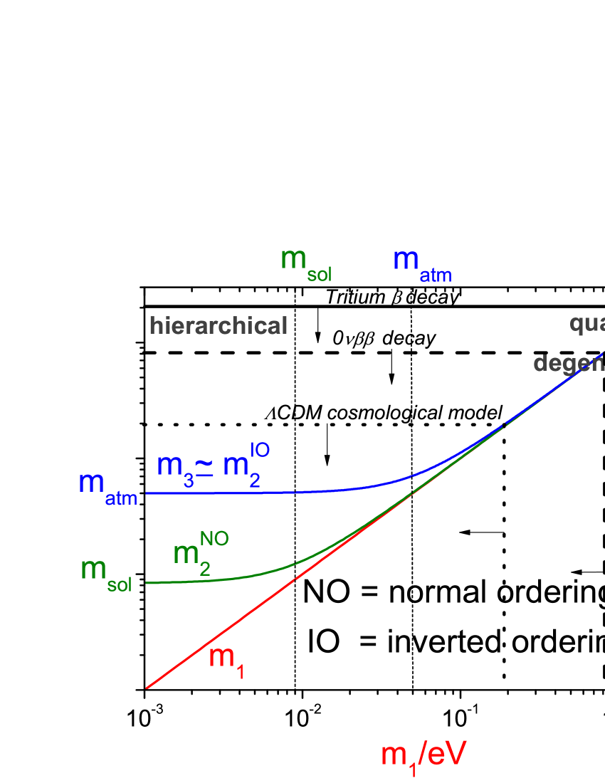
(a)

Figure 1: Neutrino masses $m_{i}$ versus the lightest neutrino mass $m_{1}$. The three upper bounds (at $95\%C.L.$) discussed in the body text from absolute neutrino mass scales phenomenologies are also indicated.

As we discussed, from cosmological observations, within the $\Lambda$CDM model, one obtains a very stringent upper bound on the sum of the neutrino masses eq. (1) that translates into the most stringent upper bound that we currently have on the lightest neutrino mass $m_{1}\lesssim 0.19\,{\rm eV}(95\%C.L.)$, almost excluding quasi-degenerate neutrino models.

3.2 Theory: the see-saw mechanism

A minimal extension of the SM able to explain not only why neutrino are massive but also why they are much lighter than all the other fermions, is given by the see-saw mechanism [5]. The SM is a quantum field theory [19]. All physical laws can ultimately be extracted by a fundamental object that is the Lagrangian, exactly like in classical systems . The difference is that while in classical systems the fundamental entities are either point-like massive particles or classical fields (e.g. the electromagnetic field), in a quantum field theory there is only one kind of fundamental entities, the quantum fields. These are operators acting on the quantum states. The quantum states that correspond to the excitations of the quantum fields correspond to the free elementary particles. In this way both matter and radiation are described in the same way.

The Lagrangian contains not only (kinetic) terms describing the evolution of the free fields but also terms describing interactions among fields. These terms are not arbitrary but emerge once particular ‘symmetries’ are imposed on the Lagrangian. In modern quantum field theories the symmetries are elements of a ‘gauge group’ and the SM is based on symmetries of a non-abelian gauge group called $SU(3)\times SU(2)\times U(1)$. Within the SM, neutrinos play quite a special role since they are massless and since they can have only one helicity, the left-handed one . This means that their spin vector always points opposite to the direction of motion (while for the anti-neutrinos is the other way around). Therefore, in the SM lagrangian there are no right-handed (RH) neutrinos (and no left-handed (LH) anti-neutrinos).

In a minimal version of the see-saw mechanism one adds $N$ RH neutrinos $N_{iR}$ to the SM lagrangian $\mathcal{L}_{\rm SM}$ . These RH neutrinos can interact with the SM leptons through so called Yukawa interactions described by a complex matrix $h$ called the Yukawa coupling matrix. At the same time one can also add a so called right-right Majorana mass term that violates lepton number and that is described by another complex matrix, the Majorana mass matrix $M$. In this way the see-saw lagrangian can be written as

$$\mathcal{L}=\mathcal{L}_{\rm SM}+i\sum_{i}\overline{N_{iR}}\gamma_{\mu}\partial^{\mu}N_{iR}-\sum_{\alpha,i}\overline{\ell_{\alpha L}}\,h_{\alpha i}\,N_{iR}\,{\phi}-{1\over 2}\,\sum_{i,j}\overline{N_{iR}^{c}}\,M_{ij}\,N_{jR}+h.c.\,,$$ (9)

where $\alpha=e,\mu,\tau$ and $i,j=1,\dots,N$ and ‘h.c.’ denotes hermitian conjugated terms. In this equation the ${\ell}_{\alpha L}$’s denote the fields associated to the so called lepton doublets (one for each flavour $\alpha$), each including one charged lepton $\alpha$ (electrons, muons and tauons) and one neutrino $\nu_{\alpha}$, while the symbol $\phi$ denotes the Higgs field.

We do not know in general the number $N$ of RH neutrinos. We just know that, in order to reproduce correctly the observed neutrino masses and mixing parameters with the see-saw mechanism that we are going to discuss in a moment, we need at least two RH neutrinos (i.e. $N\geq 2$). For definiteness we will consider the case $N=3$. This is most attractive case corresponding to have one RH neutrino for each generation in the SM, as, for example, nicely predicted by $SO(10)$ grand-unified models . Notice, however, that all current data from low energy neutrino experiments are also consistent with a more minimal two RH neutrino model, as we will discuss in more detail.

The addition of RH neutrinos in the Lagrangian with Yukawa couplings $h$ to leptons, follows exactly the same recipe that allows all massive fermions in the SM to acquire a mass through the so called Higgs mechanism. Below a certain critical temperature the neutral Higgs field acquires a non zero vacuum expectation value $v$ that breaks the electroweak symmetry of the theory and acts as a background Higgs field that fills the whole space. This is analogous to what happens in ferromagnets where below a certain critical temperature there is a non-vanishing magnetic field that breaks rotational symmetry. This spontaneous electroweak symmetry breaking results in fermion masses due to their interaction with the Higgs background field $v$. The mechanism requires the existence of RH particles. Therefore, in the SM, neutrinos do not acquire any mass simply because they do not couple to $v$. However, when RH neutrinos are added with Yukawa couplings $h$ to $v$, a neutrino Dirac mass term $m_{D}=v\,h$ is generated as for all the other massive fermions. If this were the whole story, one could easily understand why neutrinos are massive but not why they are orders-of-magnitude lighter than all the other particles. However, there is another element to be considered. Differently from all the other massive fermions, neutrinos are neutral and in general the Majorana mass term in the Lagrangian eq. (9) is also present. In this way the neutrino masses that we measure would be the result of an interplay between the usual Dirac neutrino mass term and the Majorana neutrino mass term.

Indeed one can show that in the so called ‘see-saw limit’, for $M\gg m_{D}$ , the spectrum of (ordinary) neutrino masses splits into a light set given by the eigenvalues $m_{1}<m_{2}<m_{3}$ of the neutrino mass matrix

$$m_{\nu}=-m_{D}\,{1\over M}\,m_{D}^{T}\,$$ (10)

and into a (new) heavy set coinciding with very good approximation with the eigenvalues $M_{1}<M_{2}<M_{3}$ of the Majorana mass matrix $M$ and corresponding to eigenstates $N_{i}\simeq N_{iR}$. Notice that in this formula ${1\over M}\equiv M^{-1}$. This notation emphasises the pictorial ‘see-saw’ analogy (see Fig. 2).

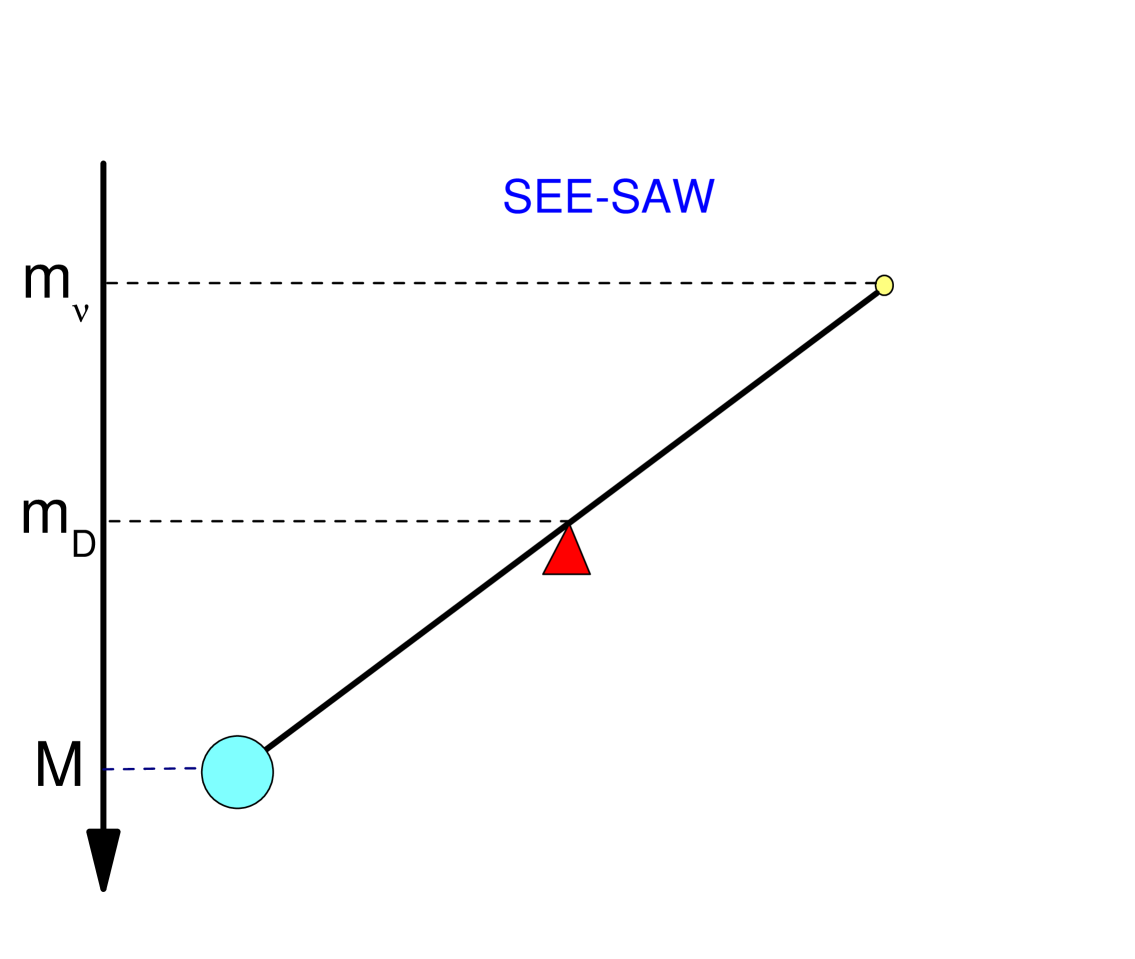
(a)

Figure 2: A pictorial representation of the see-saw formula eq. (10). The large Majorana mass scale $M$, related to some new physics scale like for example the grand-unified scale $M_{GUT}$, pushes up the light neutrino mass scale pivoting on $m_{D}$.

Consider indeed a toy model case where there is only one neutrino mass scale (it can be regarded as an approximation limit case for $m_{\rm sol}/m_{\rm atm}\rightarrow 0$) and all matrices reduces to simple numbers. If one chooses for the neutrino Dirac mass a value $m_{D}\sim v\sim 100\,{\rm GeV}$, the electroweak scale dictating the masses of all other fermions, then one can see that the atmospheric neutrino mass scale $m_{\rm atm}$ is reproduced for a value of $M\sim 10^{14-15}\,{\rm GeV}$, intriguingly very close (order-of-magnitude wise) to the grand-unified scale $M_{GUT}\sim 10^{15-16}\,{\rm GeV}$: as in a see-saw, the huge RH neutrino mass $M$, ‘sitting downstairs’ in the see-saw formula (10) and pivoting on $m_{D}$, is able to push down the light neutrino mass $m_{\nu}$.

It should then be noticed a very important implication of the see-saw mechanism: the light neutrino mass scale is not a fundamental scale, but an algebraic by-product of the combination of two much bigger scales. Within this picture, neutrino physics becomes then a portal, at low energies, of new physics at very high energies.

If we now consider the realistic case with three neutrino masses, the $(3\times 3)$ symmetric neutrino mass matrix $m_{\nu}$ is diagonalised by a unitary matrix $U$, explicitly

$$D_{m}\equiv{\rm diag}(m_{1},m_{2},m_{3})=-U_{\nu}^{\dagger}\,m_{\nu}\,U_{\nu}^{\star}\,.$$ (11)

For all practical purposes, the matrix $U_{\nu}$ here can be assumed to coincide with the leptonic mixing matrix $U$ defined in the eq.(5). The masses of the RH neutrinos are very model dependent. However it is fair to say that in order to reproduce the measured light neutrino mass scales and barring fine tuned choices of the parameters, typical proposed models give an heaviest RH neutrino mass $M_{3}\gtrsim 10^{14}\,{\rm GeV}$. This is the minimal version of the see-saw mechanism, often indicated as type I see-saw mechanism.

The see-saw formula eq. (10) can be recast as an orthogonality condition for a matrix $\Omega$ that, in a basis where simultaneously the charged lepton mass matrix and the Majorana mass matrix are diagonal, provides a useful parametrisation of the neutrino Dirac mass matrix [20],

$$m_{D}=U\,D_{m}^{1/2}\,\Omega\,D_{M}^{1/2}\,,$$ (12)

where we defined $D_{m}\equiv{\rm diag}(m_{1},m_{2},m_{3})$ and $D_{M}\equiv{\rm diag}(M_{1},M_{2},M_{3})$. The orthogonal matrix $\Omega$ encodes the properties of the heavy RH neutrinos, the three life times and the three total $C\!P$ asymmetries. This parametrisation is quite useful since, given a model that specifies $m_{D}$ and the three RH neutrino masses $M_{i}$, through it one can easily impose both the experimental information on the $9$ low energy neutrino parameters in $U$ and $m_{i}$ and, as we will see, also the requirement of successful leptogenesis.

4 The simplest scenario of leptogenesis: vanilla leptogenesis

In the most general approach the asymmetry depends on all the 18 see-saw parameters that can be identified with nine low energy parameters (three light neutrino masses plus the six parameters in the leptonic mixing matrix) and nine high energy neutrino parameters associated to the three RH neutrino properties (masses, lifetimes and total $C\!P$ asymmetries). Moreover the calculation itself presents different technical difficulties. However, there is a simplified scenario [4, 21, 22] that grasps most of the main features of leptogenesis and is able to highlight important connections with the low energy neutrino parameters in an approximated way. We will refer to this scenario as ‘vanilla leptogenesis’. We discuss the main features, assumptions and approximations. The discussion can be conveniently split into two parts: in the first part we discuss how the abundance of the RH neutrinos is calculated during the expansion of the Universe, while in the second part we describe how the baryon asymmetry is calculated.

4.1 Assumptions of minimal leptogenesis

Leptogenesis belongs to a class of models of baryogenesis where the asymmetry is generated from the out-of-equilibrium decays of very heavy particles, quite interestingly the same class as the first model proposed by Sakharov belongs. This class of models became very popular with the advent of grand-unified theories (GUTs) that provided a specific well definite and motivated framework. In GUT baryogenesis models the very heavy particles are the same new gauge bosons predicted by GUTs. However, the final asymmetry depends on too many untestable parameters, so that imposing successful baryogenesis does not lead to compelling experimental predictions. This lack of predictability is made even stronger considering that the decaying particles are too heavy to be produced thermally and one has therefore to invoke a non-thermal production mechanism of the gauge bosons. This is because while the mass of the gauge bosons is about the grandunification scale, $M_{X}\sim 10^{15-16}\,{\rm GeV}$, the reheating temperature at the end of inflation $T_{RH}$ cannot be higher than $\sim 10^{15}\,{\rm GeV}$ from CMB observations. The reheating temperature is the initial value of the temperature at the beginning of the radiation dominated regime after Inflation. Below this temperature the inflationary stage can, therefore, be considered concluded.

The minimal (and original) version of leptogenesis is based on the type I see-saw mechanism and the asymmetry is produced by the three heavy RH neutrinos. We will call ‘minimal leptogenesis scenarios’ those scenarios where a type I see-saw mechanism and a thermal production of the RH neutrinos (thermal leptogenesis), implying that $T_{RH}$ is comparable at least to the lightest RH neutrino mass $M_{1}$, are assumed. At these high temperatures the RH neutrinos can be produced by the Yukawa interactions of leptons and Higgs bosons in the thermal bath. Since in most models of neutrino masses embedding the type I see-saw mechanism the lightest RH neutrino mass $M_{1}\ll 10^{15}\,{\rm GeV}$, the condition of thermal leptogenesis can, therefore, be satisfied compatibly with the above-mentioned upper bound, $T_{RH}\lesssim 10^{15}\,{\rm GeV}$, from CMB observations.

After their production, the RH neutrinos decay either into leptons $N_{i}\rightarrow{\ell}_{i}+\phi^{\dagger}$, with a decay rate $\Gamma_{i}$, or into anti-leptons and Higgs bosons $N_{i}\rightarrow\bar{\ell}_{i}+\phi$, with a decay rate $\bar{\Gamma}_{i}$. Notice that here the leptons ${\ell}_{i}$ and the anti-leptons $\bar{\ell}_{i}$ are by definition the leptons and the anti-leptons produced by the decays of the RH neutrinos. In general, as we will discuss in detail later on, they are described by quantum states that are a linear combination of the flavour eigenstates describing the leptons ${\ell}_{\alpha}$ ($\alpha=e,\mu,\tau$) associated to the left-handed lepton doublet fields ${\ell}_{\alpha L}$ written in the lagrangian eq. (9). Since both the RH neutrinos $N_{i}$ and the Higgs bosons $\phi$ do not carry lepton number, both inverse processes and decays violate lepton number ($|\Delta L|=1$) and in general $C\!P$ as well. It is also important to notice that they also violate the $B-L$ number, ($|\Delta(B-L)|=1$). At temperatures $T\gg 100\,{\rm GeV}$ non perturbative SM processes called sphalerons are in equilibrium. They violate both lepton and baryon number while they still conserve the $B-L$ asymmetry. In this way the lepton asymmetry produced in the elementary processes is reprocessed in a way that at the end approximately $1/3$ of the $B-L$ asymmetry is in the form of a baryon asymmetry and $-2/3$ of the $B-L$ asymmetry is in the form of a lepton number: two Sakharov conditions are, therefore, clearly satisfied. The third Sakharov condition, the departure from thermal equilibrium, is also satisfied since some fraction of the decays occurs out-of-equilibrium. In this way part of the generated asymmetry survives to the wash-out from inverse processes.

4.2 Calculation of the RH neutrino abundances

In the calculation of the RH neutrino abundances a key role is played by the decay parameters $K_{i}$. They are defined as the ratio of the total decay width of the RH neutrinos $N_{i}$, $\widetilde{\Gamma}_{i}\equiv(\Gamma_{i}+\bar{\Gamma}_{i})_{T\ll M_{i}}$, to the (Hubble) expansion rate of the Universe $H$ at $T=M_{i}$, when the $N_{i}$’s start to become non-relativistic , explicitly

$$K_{i}\equiv{\widetilde{\Gamma}_{i}\over H(T=M_{i})}\,.$$ (13)

Considering that the age of the Universe is given by $t=H^{-1}/2$, while the life-times of the RH neutrinos, by definition, are given by $\tau_{i}=\widetilde{\Gamma}_{i}^{-1}$, the decay parameters can also be regarded as a ratio between the age of the Universe when they become non-relativistic, $t(T=M_{i})$, and the $\tau_{i}$’s. Therefore, for $K_{i}\gg 1$, the RH neutrinos life-time is much shorter than $t(T=M_{i})$ and they (on average) decay and inverse-decay many times before they become non-relativistic. In this situation the RH neutrino abundance tracks very closely the equilibrium distribution. On the other hand, for $K_{i}\ll 1$, the bulk of the RH neutrinos will decay completely out-of-equilibrium, when they are already fully non-relativistic and their equilibrium abundance is exponentially suppressed by the Boltzmann factor.

A quantitative calculation of the RH neutrino abundances (and also of the baryon asymmetry as we will discuss in the next subsection) requires a kinetic description. In the ‘vanilla scenario’ this is done with the use of Boltzmann equations averaged over momenta (often called ‘rate equations’). Let us indicate with $N_{N_{i}}$ the RH neutrino abundances and with $N_{N_{i}}^{\rm eq}$ their thermal equilibrium values. The Boltzmann equations for the $N_{N_{i}}$’s are then given by

$${dN_{N_{i}}\over dz}=-D_{i}\,(N_{N_{i}}-N_{N_{i}}^{\rm eq})\,,$$ (14)

where $z\equiv M_{1}/T$. Notice that we are calculating the abundance $N_{X}$ of any particle number or asymmetry $X$ in a portion of co-moving volume containing one heavy neutrino in ultra-relativistic thermal equilibrium, so that $N^{\rm eq}_{N_{i}}(T\gg M_{i})=1$.

Inroducing $x_{i}\equiv M_{i}^{2}/M_{1}^{2}$, the decay factors $D_{i}$ are defined as

$$D_{i}\equiv{\Gamma_{{\rm D},i}\over H\,z}=K_{i}\,x_{i}\,z\,\left\langle{1\over\gamma_{i}}\right\rangle\,,$$ (15)

where $H$ is the expansion rate. The total decay rates, $\Gamma_{{\rm D},i}\equiv\Gamma_{i}+\bar{\Gamma}_{i}$, are the product of the decay widths $\widetilde{\Gamma}_{i}$ times the thermally averaged dilation factors $\langle 1/\gamma\rangle$, given by the ratio ${\cal K}_{1}(z)/{\cal K}_{2}(z)$ of the modified Bessel functions. It should be noticed how for each RH neutrino species $N_{i}$, the associated decay parameter $K_{i}$ is the only parameter that determines its abundance $N_{N_{i}}$ in addition to the initial value $N_{N_{i}}^{\rm in}$.

In Fig. 3 we show the result for the lightest RH neutrino abundance $N_{N_{1}}$ and for the two cases $K_{1}=10^{-2}\ll 1$ and $K_{1}=10\gg 1$. The initial RH neutrino abundance $N_{N_{1}}^{\rm in}$, typically at some $z_{\rm in}\ll 1$, is in general an unknown parameters and it has been here chosen equal to the thermal equilibrium value. It can be clearly seen how in the first case the equilibrium abundance closely tracks the equilibrium value, while in the second case there is a clear departure from thermal equilibrium.

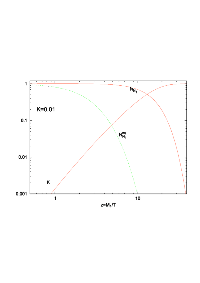
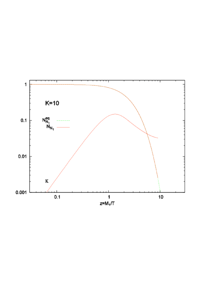
Figure 3: Evolution of the RH neutrino abundance $N_{N_{1}}$ (red line) and of the efficiency factor $\kappa$ (red line) with the temperature for two different values of the decay parameter $K_{1}$: (left) $K_{1}=0.01$ and (right) $K_{1}=10$. The green dotted line is the thermal equilibrium abundance $N_{N_{1}}^{\rm eq}$: in the right panel it is hardly visible since it is closely tracked by $N_{N_{1}}$.

4.3 Calculation of the baryon asymmetry

Let us now turn to discuss how the baryon asymmetry is calculated in the vanilla scenario. The flavour composition of the leptons ${\ell}_{i}$ and anti-leptons $\bar{\ell}_{i}$ produced by (or producing) the RH neutrinos is assumed to have no influence on the final value of the asymmetry and is therefore neglected (assumption of ‘unflavoured’ or ‘one-flavoured’ leptogenesis). This is equivalent to say that the only relevant quantity is the total lepton asymmetry, i.e. the difference between the total number of leptons and the total number of anti-leptons irrespectively whether these leptons are electron, muon or tauon doublets (at these temperatures the electroweak symmetry is not broken). As we said at very high temperatures $T\gg 100\,{\rm GeV}$, part of the total lepton asymmetry is rapidly converted into a baryon asymmetry by sphaleron processes. However sphaleron processes conserve the $B-L$ asymmetry and it can be shown that at the end approximately the final baryon asymmetry $N_{B}^{\rm f}\simeq N_{B-L}^{\rm f}/3$ while the final lepton asymmetry $N^{\rm f}_{L}\simeq-2\,N_{B-L}^{\rm f}/3$.

For this reason it is convenient to track the $B-L$ asymmetry and not the individual lepton or baryon asymmetry. The evolution of $B-L$ asymmetry is described by the following Boltzmann (rate) equation

$${dN_{B-L}\over dz}=\sum_{i=1}^{3}\,\varepsilon_{i}\,D_{i}\,(N_{N_{i}}-N_{N_{i}}^{\rm eq})-N_{B-L}\,[\Delta W(z)+\sum_{i}\,W_{i}^{\rm ID}(z)]\;,$$ (16)

that can be solved as a coupled equation together with the Boltzmann equations for the RH neutrino abundances eqs. (14). The first term in the right-hand side is a source term for the asymmetry and is proportional to the three total $C\!P$ asymmetries defined as

$$\varepsilon_{i}\equiv-{\Gamma_{i}-\bar{\Gamma}_{i}\over\Gamma_{i}+\bar{\Gamma}_{i}}\,,$$ (17)

corresponding to the $B-L$ asymmetry produced, on average, by each single $N_{i}$ decay. A perturbative calculation from the interference of tree level with one loop self-energy and vertex diagrams (see Fig. 4), gives [23]

$$\varepsilon_{i}=\,{3\over 16\pi}\,\sum_{j\neq i}\,{{\rm Im}\,\left[(h^{\dagger}\,h)^{2}_{ij}\right]\over(h^{\dagger}\,h)_{ii}}\,{\xi(x_{j}/x_{i})\over\sqrt{x_{j}/x_{i}}}\,,$$ (18)

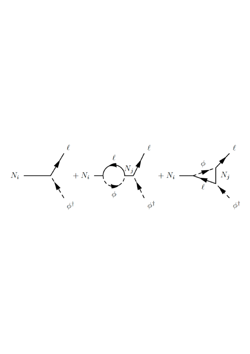
Figure 4: The Feynman diagrams that are employed in the calculation of the expression of the $C\!P$ asymmetry eq. (18): tree level diagram (left), one loop self energy diagram (centre), one loop vertex diagram (right).

where

$$\xi(x)={2\over 3}\,x\,\left[(1+x)\,\ln\left({1+x\over x}\right)-{2-x\over 1-x}\right]\,.$$ (19)

If it were not for the interference, in a pure tree level calculation, one would obtain $\Gamma_{i}=\bar{\Gamma}_{i}$.

The second term in the right-hand side of the eq. (16) is the so called wash-out term. It is a term that tends to re-equilibrate the number of leptons and anti-leptons destroying the asymmetry created by the source $C\!P$ violating term. Differently from that term, it does not depend at all on the $C\!P$ asymmetries and it is present even if these vanish. It is simply a statistical re-equilibrating term that has to be present in order for the third Sakharov condition, on the departure from thermal equilibrium, to be respected. This is because if there is no (permanent) departure from thermal equilibrium, this term would destroy completely any asymmetry previously generated.

The wash-out term is proportional to the wash-out factor that is composed of two terms: a term $\sum_{i}W_{i}^{\rm ID}(z)$ due to inverse decays (i.e. ${\ell}_{i}\,(\bar{\ell}_{i})+\phi^{\dagger}\,(\phi)\rightarrow N_{i}$) and a term $\Delta W(z)$ due to (non-resonant) $\Delta L=2$ processes (${\ell}_{i}+\phi^{\dagger}\leftrightarrow\bar{\ell}_{i}+\phi$). After proper subtraction of the resonant contribution from $\Delta L=2$ processes, the inverse decay washout terms are simply given by

$$W_{i}^{\rm ID}(z)={1\over 4}\,K_{i}\,\sqrt{x_{i}}\,{\cal K}_{1}(z_{i})\,z_{i}^{3}\,,$$ (20)

where $z_{i}\equiv z\,\sqrt{x_{i}}$. The washout term $\Delta W(z)$ gives a non-negligible effect only at $z\gg 1$ and in this case it can be approximated as [21]

$$\Delta W(z)\simeq{\omega\over z^{2}}\,\left(M_{1}\over 10^{10}\,{\rm GeV}\right)\,\left({\overline{m}^{\,2}\over{\rm eV^{2}}}\right)\,,$$ (21)

where $\omega\simeq 0.186$ and $\overline{m}^{2}\equiv m_{1}^{2}+m_{2}^{2}+m_{3}^{2}$.

The solution of the Boltzmann equations for the final $B-L$ asymmetry can be written as the sum of two contributions,

$$N^{\rm f}_{B-L}=N^{\rm pre-ex,f}_{B-L}+N^{\rm lep,f}_{B-L}\,.$$ (22)

The first term, $N^{\rm pre-ex,f}_{B-L}$, is the residual value of a possible pre-existing asymmetry generated by some external mechanism prior to the onset of leptogenesis. Therefore, it represents a possible external contribution whose initial value would originate from some source beyond leptogenesis. Therefore, if one wants to explain the observed asymmetry with leptogenesis, this term has to be negligible.

The second term is the genuine leptogenesis contribution to the final asymmetry and is the sum of three contributions, one for each RH neutrino species,

$$N^{\rm lep,f}_{B-L}=\sum_{i}\,\varepsilon_{i}\,\kappa_{i}^{\rm f}(K_{1},K_{2},K_{3})\,.$$ (23)

Each contribution is the product of the total $C\!P$ asymmetry $\varepsilon_{i}$ times the final value of the efficiency factor, $\kappa_{i}^{\rm f}(K_{i})$, depending on the decay parameter $K_{i}$. The efficiency factors can be simply calculated analytically as

$$\kappa_{i}(z;K_{i})=-\int_{z_{\rm in}}^{z}\,dz^{\prime}\,{dN_{N_{i}}\over dz^{\prime}}\,{\rm e}^{-z^{\prime}\,\Delta W(z^{\prime})+\sum_{i}\,\int_{z^{\prime}}^{\infty}\,dz^{\prime\prime}\,W_{i}^{\rm ID}(z^{\prime\prime};K_{i})]}$$ (24)

and their final values $\kappa_{i}^{\rm f}(K_{i})=\kappa_{i}(z=\infty;K_{i})$. Finally, the predicted baryon-to-photon ratio $\eta_{B}$ can be calculated from the final value of the final $B-L$ asymmetry using the relation

$$\eta_{B}^{\rm lep}=a_{\rm sph}{N_{B-L}^{\rm lep,f}\over N_{\gamma}^{\rm rec}}\simeq 0.96\times 10^{-2}N_{B-L}^{\rm f}\,,$$ (25)

where $N_{\gamma}^{\rm rec}\simeq 37$, and $a_{\rm sph}=28/79\simeq 1/3$. The factor $1/N_{\gamma}^{\rm rec}$ takes into account the photon production after leptogenesis, due to the annihilations of SM particles, that has the effect to dilute the asymmetry with respect to the number of photons. The factor $a_{\rm sph}$ is the fraction of the $B-L$ asymmetry ending up into a baryon asymmetry under the action of sphaleron processes. The condition of successful leptogenesis corresponds to impose that $\eta_{B}^{\rm lep}$ reproduces the measured value of $\eta_{B}^{CMB}$ (cf. eq. (4)).

There is a second important assumption within the vanilla scenario in the calculation of the baryon asymmetry: the RH neutrino mass spectrum is assumed to be hierarchical with $M_{2}\gtrsim 3\,M_{1}$. Together with the assumption of unflavoured leptogenesis, the final asymmetry is in this case dominantly produced by the lightest RH neutrino out-of-equilibrium decays, in a way that the sum in the eq. (22) can be approximated by the first term ($i=1$), explicitly

$$N_{B-L}^{\rm f}\simeq\varepsilon_{1}\,\kappa_{1}^{\rm f}(K_{1})\,,$$ (26)

and a ‘$N_{1}$-dominated scenario’ holds. In Fig. 3 we show a calculation of $\kappa^{\rm f}(K_{1})$ for $K_{1}=0.01$ (weak wash-out regime) and for $K_{1}=10$ (strong wash-out regime) and for initial thermal abundance ($N_{N_{1}}^{\rm in}=1$). In the first case all the asymmetry produced in the decays of the RH neutrino survives and $\kappa_{1}^{\rm f}=N^{\rm in}_{N_{1}}=1$. In the second case only a small fraction of the asymmetry survives and $\kappa_{1}^{\rm f}\simeq 0.01$, still however large enough to reproduce successfully the observed asymmetry if $\varepsilon_{1}\simeq 10^{-6}$.

The ‘$N_{1}$-dominated scenario’ holds either because $|\varepsilon_{2,3}|\ll|\varepsilon_{1}|$ and/or because the asymmetry initially produced by the $N_{2,3}$ decays is afterwards washed-out by the lightest RH neutrino inverse processes in a way that $\kappa_{2,3}^{\rm f}\ll\kappa_{1}^{\rm f}$. Indeed if we indicate with $N_{B-L}^{(2,3)}(T\gtrsim M_{1})$ the contribution to the $N_{B-L}$ asymmetry from the two heavier RH neutrinos prior to the lightest RH neutrino wash-out, the final values are given very simply by

$$N_{B-L}^{(2,3),{\rm f}}=N_{B-L}^{(2,3)}(T\gtrsim M_{1})\,e^{-{3\pi\over 8}\,K_{1}}\,.$$ (27)

The same exponential wash-out factor applies to the residual value of a possible pre-existing asymmetry. In this way it is sufficient to have a strong wash-out condition $K_{1}\gg 1$ in order to have both a pre-existing asymmetry and a contribution from heavier RH neutrinos negligible. The strong wash-out condition $K_{1}\gg 1$ is very easily satisfied since, barring special cases, one has typically $K_{1}\simeq(m_{\rm sol}\div m_{\rm atm})/10^{-3}\,{\rm eV}\gg 1$. The same condition also guarantees independence of the final asymmetry on the initial $N_{1}$-abundance. It is then quite suggestive that the measured values of $m_{\rm sol}$ and $m_{\rm atm}$ have just the right values to produce a wash-out that is strong enough to guarantee independence on the initial conditions but still not too strong to prevent successful leptogenesis. This leptogenesis conspiracy between experimental results and theoretical prediction is one of the main reasons that has determined the success of leptogenesis so far.

There is actually a particular case where $K_{1}\gg 1$ and $|\varepsilon_{2}|\ll|\varepsilon_{1}|$ do not hold and in this case the final asymmetry is dominated by the contribution coming from the next-to-lightest RH neutrinos. However, one still has $K_{2}\gg 1$ so that the independence of the initial conditions still holds. For the time being, as an additional third assumption of the vanilla scenario, we will bar this particular case, we will be back on it in 3.1.

If, additionally, one excludes fine tuned cancelations among the different terms contributing to the neutrino masses in the see-saw formula, one obtains the following upper bound on the lightest RH neutrino $C\!P$ asymmetry [24]

$$\varepsilon_{1}\leq\varepsilon_{1}^{\rm max}\simeq 10^{-6}\,{M_{1}\over 10^{10}\,{\rm GeV}}\,{m_{\rm atm}\over m_{1}+m_{3}}\,.$$ (28)

Imposing $\eta_{B}^{\rm max}\simeq 0.01\,\varepsilon_{1}^{\rm max}\,\kappa_{1}^{\rm f}>\eta_{B}^{CMB}$, one obtains the allowed region in the plane $(m_{1},M_{1})$ shown in the left panel of Fig. 5.

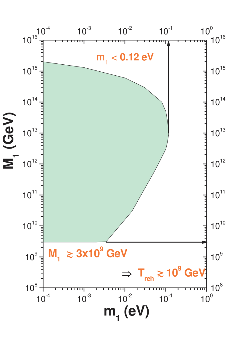
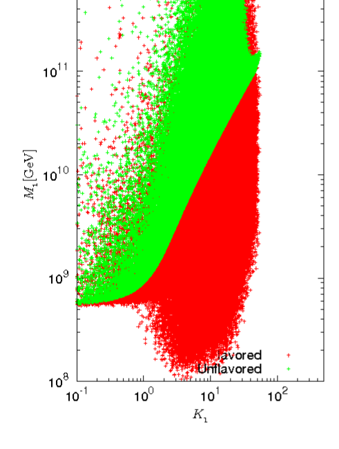
Figure 5: Left: Neutrino mass bounds in the vanilla scenario. Right: Relaxation of the lower bound on $M_{1}$ thanks to additional unbounded flavoured $C\!P$ violating terms.

One can notice the existence of an upper bound on the light neutrino masses $m_{1}\lesssim 0.12\,{\rm eV}$ [21], incompatible with quasi-degenerate neutrino mass models, and a lower bound on $M_{1}\gtrsim 3\times 10^{9}\,{\rm GeV}$ [24, 21] implying a lower bound on the reheat temperature $T_{\rm RH}\gtrsim 10^{9}\,{\rm GeV}$ [21].

An important feature of vanilla leptogenesis is that the final asymmetry does not directly depend on the parameters of leptonic mixing matrix $U$. This implies that one cannot establish a direct model independent connection. In particular a discovery of CP violation in neutrino mixing would not be a smoking gun for leptogenesis and, vice versa, a non-discovery would not rule out leptogenesis. However, within more restricted scenarios, for example imposing some conditions on the neutrino Dirac mass matrix, links can emerge. We will discuss in detail the interesting case of $SO(10)$-inspired models.

5 Beyond vanilla leptogenesis

In the last years different directions beyond the vanilla leptogenesis scenario have been explored, usually aiming at evading the above-mentioned bounds. The most important one is certainly the inclusion of flavour effects and for this reason we will discuss them in detail in the next Section. In this section we briefly mention other important extensions of the vanilla scenario that have been considered and studied.

5.1 Beyond a hierarchical RH neutrino mass spectrum

If $(M_{2}-M_{1})/M_{1}\equiv\delta_{2}\ll 1$, the $C\!P$ asymmetries $\varepsilon_{1,2}$ get resonantly enhanced as $\varepsilon_{1,2}\propto 1/\delta_{2}$ [23]. If, more stringently, $\delta_{2}\lesssim 10^{-2}$, then $\eta_{B}\propto 1/\delta_{2}$ and the degenerate limit is obtained [25]. In this limit the lower bounds on $M_{1}$ and on $T_{\rm RH}$ get relaxed $\propto\delta_{2}$ and at the resonance they completely disappear [26]. However, there are not many models able to justify in a reasonable way such a very closely degenerate limit yielding resonant leptogenesis.

5.2 Non minimal leptogenesis

Other proposals to relax the lower bounds on $M_{1}$ and on $T_{RH}$ rely on extensions beyond minimal leptogenesis. For example a popular scenario relies on the addition of a so called left-left Majorana mass term to the lagrangian (9). However, this implies that the existence of new particles, beyond the SM particles and RH neutrinos, has to be postulated since otherwise it would not be possible to write such a term preserving the symmetries of the lagrangian. The most popular way is to include a new kind of Higgs boson, $\Delta$ with mass $M_{\Delta}$, with different properties than the SM Higgs boson. In this way one can show that in the see-saw formula eq. (10) for the neutrino masses a second term appears. This term is $\propto(v^{2}/M_{\Delta})\times I$, where $I$ is the identity matrix. This extension of the seesaw mechanism is called type II see-saw mechanism [27] and it is particularly suitable to describe quasi-degenerate neutrino masses. However, as shown in Fig. 1, these start to be strongly constrained by cosmology and a simple type II extension does not seem strictly necessary within the current experimental results.

Another popular way to go beyond a minimal scenario of leptogenesis relies on a non thermal production of the RH neutrinos generating the asymmetry [28]. However, these non minimal models spoil somehow the remarkable coincidence between the measured values of the atmospheric and solar neutrino mass scales and the possibility to have successful leptogenesis with $\eta_{B}\sim 10^{-9}$ even independently of the initial conditions. Non-minimal models have been also extensively recently explored in order to get a low scale leptogenesis testable at colliders [29].

5.3 Improved kinetic description

Within vanilla leptogenesis the asymmetry is calculated solving simple rate equations, classical Boltzmann equations integrated over the RH neutrino momenta. Different kinds of extensions have been studied [30], for example accounting for $\Delta L=1$ scatterings, momentum dependence, quantum kinetic effects and thermal effects. All these analyses find significant changes in the weak wash-out regime but within ${\cal O}(1)$ in the strong wash-out regime. This result has quite a straightforward general explanation [21]. In the strong wash-out regime the final asymmetry is produced by the decays of RH neutrinos in a non relativistic regime when a simple classical momentum independent kinetic description provides quite a good approximation. The use of a simple kinetic description in leptogenesis is therefore not just a simplistic approach but is justified in terms of the neutrino oscillation experimental results on the neutrino masses that support a strong wash-out regime with $K_{i}\gg 1$.

6 The importance of flavour

In the last years, the inclusion of flavour effects in the calculation of the final asymmetry proved to yield the most significant changes to the calculation of the final asymmetry going beyond the vanilla scenario.

There are two kinds of flavour effects that are neglected in the vanilla scenario: heavy neutrino flavour effects [31], how heavier RH neutrinos contribute to the final asymmetry, and lepton flavour effects [32, 33], how the flavour composition of the leptons quantum states produced in the RH neutrino decays affects the calculation of the final asymmetry. We first discuss the two effects separately and then we show how their interplay has very interesting consequences.

6.1 Heavy neutrino flavour effects

In the vanilla scenario the contribution to the final asymmetry from the heavier RH neutrinos is negligible because either the $C\!P$ asymmetries are suppressed in the hierarchical limit with respect to $\varepsilon_{1}^{\rm max}$ (cf. eq. (28)) and/or because even assuming that a sizeable asymmetry is produced around $T\sim M_{2,3}$, this is later on washed out by the lightest RH neutrino inverse processes.

However, as we anticipated, there is a particular case when, even neglecting the lepton flavour composition and assuming a hierarchical heavy neutrino mass spectrum, the contribution to the final asymmetry from next-to-lightest RH neutrino decays can be dominant [31]. This case corresponds to a particular choice of the orthogonal matrix such that $N_{1}$ is very weakly coupled (corresponding to have $K_{1}\ll 1$) and its wash-out can be neglected. For the same choice of the parameters, the $N_{2}$ total $C\!P$ asymmetry $\varepsilon_{2}$ is unsuppressed if $M_{3}\lesssim 10^{15}\,{\rm GeV}$. In this case a $N_{2}$-dominated scenario is realised. Notice that in this case the existence of a third heaviest RH neutrino species is crucial in order to have a sizeable $\varepsilon_{2}$.

The contribution from the next-to-lightest RH neutrino species $N_{2}$ is also important in the quasi-degenerate limit when $\delta_{2}\ll 1$. In this case the $C\!P$ asymmetries $\varepsilon_{2}$ is also not suppressed and the wash-out from the lightest RH neutrinos on the asymmetry produced by $N_{2}$ is only partial [26, 25]. Analogously, if $\delta_{3}\equiv(M_{3}-M_{1})/M_{1}\ll 1$, then the contribution to the final asymmetry from $N_{3}$ has also in general to be taken into account.

6.2 Lepton flavour effects

For the time being, let us continue to assume that the final asymmetry is dominantly produced by the contribution of the lightest RH neutrinos $N_{1}$, neglecting the contribution from the decays of the heavier RH neutrinos $N_{2}$ and $N_{3}$. If $M_{1}\gg 10^{12}\,{\rm GeV}$, the flavour composition of the quantum states of the leptons produced in $N_{1}$ decays has no influence on the final asymmetry and the ‘unflavoured regime’, assumed in the vanilla scenario, holds.

This is because for such a large $M_{1}$, the asymmetry is produced at temperatures where all the relevant interactions are flavour blind. In this way the lepton quantum states evolve coherently between the production from a $N_{1}$-decay and a subsequent inverse decay with an Higgs boson and the lepton flavour composition does not play any role in the calculation of the final asymmetry.

However, if $10^{12}\,{\rm GeV}\gtrsim M_{1}\gtrsim 10^{9}\,{\rm GeV}$, during the relevant period of generation of the asymmetry, it can be shown that the rate of the tauon lepton interactions becomes much larger than the inverse decay rate. As a consequence, the produced lepton quantum states on average, between one decay and a subsequent inverse decay, interact with tauons. In this way the tauon component of the lepton quantum states is measured by the thermal bath and the coherent evolution breaks down. Therefore, at the subsequent inverse decay, the leptonic quantum states are an incoherent mixture of a tauon component and of a (still coherent) superposition of an electron and of a muon component that we can indicate with ${\ell}_{e+\mu}$. The fraction of the asymmetry stored in each flavour component is not proportional in general to the branching ratio of that component. This implies that the two flavour asymmetries, the tauon and the $e+\mu$ components, evolve differently and have to be calculated separately. In this way the resulting final asymmetry can considerably differ from the result one would obtain in the unflavoured regime. This regime is called the ‘two fully flavoured regime’.

If $M_{1}\lesssim 10^{9}\,{\rm GeV}$, then even the coherence of the $e+\mu$ component is broken by the muon interactions between decays and inverse decays during the relevant period of generation of the asymmetry. In this situation all three flavoured asymmetries (electron, muon and tauon asymmetries) evolve independently of each other and a ‘three fully flavoured regime’ applies. In the intermediate regimes a density matrix formalism is necessary to properly describe decoherence [32, 34, 35].

It is useful to discuss explicitly how the calculation of the baryon asymmetry proceeds in the three fully flavoured regime. Defining the flavoured asymmetries as $\Delta_{\alpha}\equiv B/3-L_{\alpha}$, their abundances $N_{\Delta_{\alpha}}$, obeying $\sum_{\alpha=e,\mu,\tau}N_{\Delta_{\alpha}}=N_{B-L}$, can be calculated solving the following Boltzmann equations

$${dN_{\Delta_{\alpha}}\over dz}=\varepsilon_{1\alpha}\,D_{1}\,(N_{N_{1}}-N_{N_{1}}^{\rm eq})-p_{1\alpha}^{0}\,N_{\Delta_{\alpha}}\,W_{1}^{\rm ID}(z)\hskip 28.45274pt(\alpha=e,\mu,\tau)\;,$$ (29)

that has to be solved together with the Boltzmann equation for $N_{N_{1}}$ (cf. eq. (14)). In the first term of the right-hand side, we have a source term for the flavoured asymmetry that is proportional to the the flavoured $C\!P$ asymmetry $\varepsilon_{1\alpha}$. In general, for a given RH neutrino $N_{i}$, the flavoured $C\!P$ asymmetries are defined as

$$\varepsilon_{i\alpha}\equiv-{\Gamma_{i\alpha}-\bar{\Gamma}_{i\alpha}\over\Gamma_{i}+\bar{\Gamma}_{i}}\,,$$ (30)

where $\Gamma_{i\alpha}\equiv p_{i\alpha}\,\Gamma_{i}$ and $\bar{\Gamma}_{i\alpha}\equiv\bar{p}_{i\alpha}\,\bar{\Gamma}_{i}$ and $p_{i\alpha}$ and $\bar{p}_{i\alpha}$ are respectively the branching ratios for the decay of the RH neutrino $N_{i}$ into a lepton ${\ell}_{\alpha}$ and into an anti-lepton $\bar{\ell}_{\alpha}$.

The wash-out factor is smaller than in the unflavoured case since $W_{1}^{\rm ID}(z)$ is now replaced by $p^{0}_{1\alpha}\,W_{1}^{\rm ID}(z)$, where $p^{0}_{1\alpha}$ is the average of $p_{1\alpha}$ and $\bar{p}_{1\alpha}$. Correspondingly, it will also prove useful to define the flavoured decay parameters $K_{i\alpha}\equiv p^{0}_{i\alpha}\,K_{i}$.

The final $B-L$ asymmetry has now to be calculated as the sum of the final values of the flavoured asymmetries, $N^{\rm f}_{B-L}=\sum_{\alpha}\,N^{\rm f}_{\Delta_{\alpha}}$. Even though the kinetic equations for the $N_{\Delta_{\alpha}}$ (cf. eq. (29)) are analogous to the eq. (16) for the calculation of $N_{B-L}$ in the unflavoured regime, the final result for $\eta_{B}$ can be in general very different. The most drastic departure from the unflavoured results is the special case $\varepsilon_{1}=0$. In the vanilla scenario, assuming the unflavoured regime, this would simply yield $N^{\rm f}_{B-L}=\eta_{B}=0$, i.e. no asymmetry would be produced at all. This is in agreement with an extension of the Sakharov condition to vanilla leptogenesis that implies that $B-L$ has not to be conserved. However, in the three fully flavoured regime, this condition is too restrictive and it is enough that the $\Delta_{\alpha}$’s are not conserved in order to produced a non-vanishing baryon asymmetry.

The flavoured Boltzmann equations eqs. (29), written in the three fully flavoured regime, can be straightforwardly extended to the two fully flavoured regime: simply the equations for $\Delta_{e}$ and $\Delta_{\mu}$ are replaced by one equation for the asymmetry $\Delta_{e+\mu}\equiv\Delta_{e}+\Delta_{\mu}$, where $\varepsilon_{1e}$ and $\varepsilon_{1\mu}$ are replaced by $\varepsilon_{1,e+\mu}\equiv\varepsilon_{1e}+\varepsilon_{1\mu}$ and $K_{1e}$ and $K_{1\mu}$ are replaced by $K_{1,e+\mu}\equiv K_{1e}+K_{1\mu}$.

We can summarise the results for the calculation of the baryon asymmetry within the fully flavoured regimes (two or three) saying that lepton flavour effects induce three major consequences. i) The wash-out can be considerably lower than in the unflavoured regime [32, 33]. ii) The low energy phases affect directly the final asymmetry since they contribute to a second source of $C\!P$ violation in the flavoured $C\!P$ asymmetries [36]. As a consequence the same source of $C\!P$ violation that could take place in neutrino oscillations, could be sufficient to explain the observed asymmetry, though under quite stringent conditions on the RH neutrino mass spectrum. In the light of the recent overwhelming evidence of a non-vanishing $\theta_{13}$ angle [37], a necessary condition to have $C\!P$ violation in neutrino oscillations, this problem becomes particularly interesting, in particular a precise calculation, within a density matrix formalism, of the lower bound on $\theta_{13}$. iii) Compared to the total $C\!P$ asymmetries, the flavoured $C\!P$ asymmetries contain extra-terms that are not upper bounded if one allows for a cancelations in the see-saw formula among the light neutrino mass terms together with a mild RH neutrino mass hierarchy ($M_{2}/M_{1}\sim 10$). In this way the lower bound on $T_{RH}$ can be relaxed by about one order of magnitude, down to $10^{8}\,{\rm GeV}$ [22] as shown in the right panel of Fig. 5. However for most models, such as sequential dominated models [38], these cancellations do not occur. In this case lepton flavour effects cannot relax the lower bound on $T_{\rm RH}$.

6.3 The interplay between lepton and heavy neutrino flavour effects

As we have seen, when lepton flavour effects are neglected, the possibility that the next-to-lightest RH neutrino decays contribute to the final asymmetry is a special case. On the other hand, when lepton flavour effects are taken into account, the contribution from next-to-lightest RH neutrinos cannot be neglected in general. Even the contribution from the heaviest RH neutrinos can be sizeable in some cases and has to be taken into account in general.

Assuming hierarchical mass patterns and that the RH neutrino processes occur in one of the three fully flavoured regimes, there are 10 possible different mass patterns to consider (see Fig. 6) requiring specific multi-stage sets of classical Boltzmann equations for the calculation of the final asymmetry.

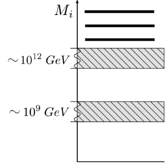
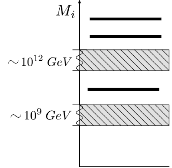
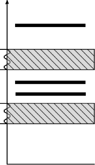
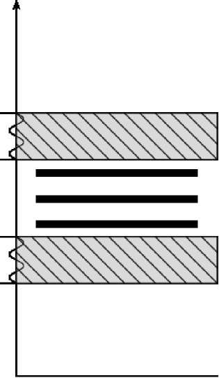
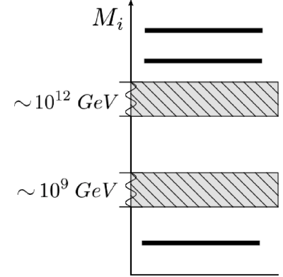
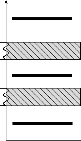
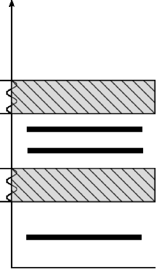
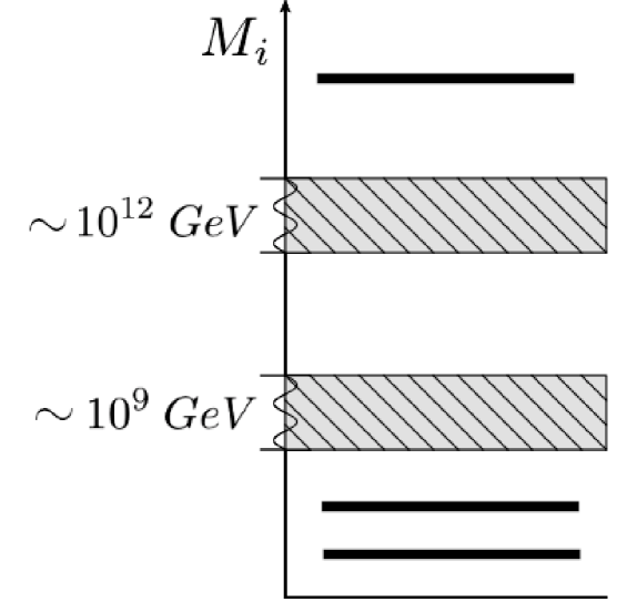
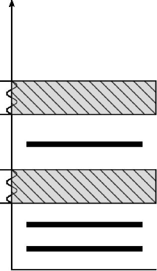
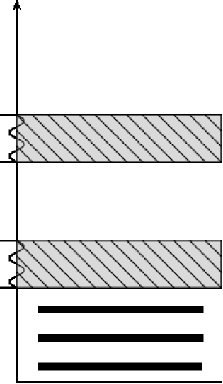
Figure 6: The 10 RH neutrino mass patterns corresponding to leptogenesis scenarios with different sets of classical Boltzmann equations for the calculation of the final asymmetry.

6.3.1 The (flavoured) $N_{2}$-dominated scenario

Among the possible 10 RH neutrino mass patterns shown in Fig. 6, for those three where the $N_{1}$ wash-out occurs in the three fully flavoured regime, for $M_{1}\ll 10^{9}\,{\rm GeV}$, the asymmetry produced by the lightest RH neutrinos is much lower than the observed value eq. (4). The reason is that for these low values of the RH neutrino masses, the flavoured $C\!P$ asymmetries of the lightest RH neutrinos are too small.

Therefore, the final asymmetry has necessarily to be produced by the heavier RH neutrinos, usually from the next-to-lightest RH neutrinos, since the $C\!P$ asymmetries of the heaviest RH neutrinos $N_{3}$ are typically suppressed. The asymmetry can be produced from the $N_{2}$’s either in the unflavoured (for $M_{2}\gg 10^{12}\,{\rm GeV}$) or in the two fully flavoured regime (for $10^{12}\,{\rm GeV}\gg M_{2}\gg 10^{9}\,{\rm GeV}$). These scenarios have some particularly attractive features and correspond to a flavoured $N_{2}$-dominated scenario [39] (it corresponds to the mass patterns (e), (f) and (g) in Fig. 6).

While within the unflavoured approximation, assumed in the vanilla scenario, the wash-out from $N_{1}$ yields a global exponential wash-out factor (cf. eq. (27)), when lepton flavour effects are taken into account the asymmetry produced by the $N_{2}$’s, at the $N_{1}$ wash-out, distributes into an incoherent mixture of lepton flavour quantum eigenstates. It turns out that the $N_{1}$ wash-out in one of the three flavours is negligible, corresponding to have at least one $K_{1\alpha}\lesssim 1$, in quite a wide region of the parameter space [22]. In this way, accounting for flavour effects, the region of applicability of the $N_{2}$-dominated scenario enlarges considerably, since it is not necessary that $N_{1}$ fully decouples but it is sufficient that it decouples just in a specific lepton flavour.

Recently, it has also been realised that, accounting for the Higgs and for the quark asymmetries, the dynamics of the flavour asymmetries couple and the lightest RH neutrino wash-out in a particular flavour can be circumvented even when $N_{1}$ is strongly coupled in that flavour [40]. Another interesting effect arising in the $N_{2}$-dominated scenario is phantom leptogenesis. This is a pure quantum-mechanical effect originating from the fact that parts of the flavoured asymmetries, the phantom terms, escape completely the wash-out at the production. These terms are proportional to the initial $N_{2}$-abundance and, therefore, introduce an additional dependence on the initial abundance of the RH neutrinos. More generally, it has been recently shown that phantom terms associated to a RH neutrino species $N_{i}$ with $M_{i}\gg 10^{9}\,{\rm GeV}$ are non-vanishing if the initial $N_{i}$ abundance is non-vanishing. However, the phantom terms produced by the lightest RH neutrinos cancel with each other and do not contribute to the final total asymmetry though they can contribute to the flavoured asymmetries and could have potential applications, for example, in active-sterile neutrino oscillations in the early Universe [35].

6.3.2 Heavy neutrino flavour projection

Even assuming a strong RH neutrino mass hierarchy, a coupled $N_{1}$ and $M_{1}\gtrsim 10^{12}\,{\rm GeV}$ (it corresponds to the first panel in Fig. 6), the asymmetry produced by the heavier RH neutrino decays, in particular by the $N_{2}$’s decays, can be sizeable and in general is not completely washed-out by the lightest RH neutrino processes. This is because there is in general an (orthogonal) component that escapes the $N_{1}$ wash-out [41] while the remaining (parallel) component undergoes the usual exponential wash-out. For a mild mass hierarchy, $\delta_{3}\lesssim 10$, even the asymmetry produced by the $N_{3}$’s decays can be sizeable and circumvent the $N_{1}$ and $N_{2}$ wash-out.

Due to this effect of heavy neutrino flavour projection and because of an additional contribution to the flavoured $C\!P$ asymmetries $\varepsilon_{2\alpha}$, that is independent of the heaviest RH neutrino mass $M_{3}$ and that is not suppressed in the hierarchical limit, it has been recently noticed that, when lepton flavour effects are consistently taken into account, the contribution from the next-to-lightest RH neutrinos can be dominant even in an effective two RH neutrino model with $M_{3}\gtrsim 10^{15}\,{\rm GeV}$ [42].

6.3.3 The problem of the initial conditions in flavoured leptogenesis

As we have seen, within an unflavoured description, as in the vanilla scenario, the problem of the dependence on the initial conditions reduces just to satisfy the strong washout condition $K_{1}\gg 1$. In other words there is a full correspondence between strong wash-out and independence of the initial conditions.

When (lepton and heavy neutrino) flavour effects are considered, the situation is much more involved and for example imposing strong wash-out conditions on all flavoured asymmetries ($K_{i\alpha}$) is not enough to guarantee independence of the initial conditions. Perhaps the most striking consequence is that in a traditional $N_{1}$-dominated scenario there is no condition that can guarantee independence of the initial conditions. The only possibility to have independence of the initial conditions is represented by a tauon $N_{2}$-dominated scenario [43], that means a scenario where the asymmetry is dominantly produced from the next-to-lightest RH neutrinos, implying $M_{2}\gg 10^{9}\,{\rm GeV}$, in the tauon flavour. The condition $M_{1}\ll 10^{9}\,{\rm GeV}$ is also important to have a projection of the quantum lepton states on the orthonormal three lepton flavour basis prior to the lightest RH neutrino wash-out.

6.3.4 Density matrix formalism

As in the case of the $N_{1}$-dominated scenario, a density matrix formalism allows to extend the calculation of the final asymmetry when the RH neutrino masses fall in one of the two transition regimes between two fully flavoured regimes. In this way, with a density matrix equation, the calculation of the final asymmetry can be performed for a generic choice of the three RH neutrino masses. Moreover within a density matrix formalism, the validity of the multi-stage Boltzmann equations describing the ten asymptotic limits shown in Fig. 6, including the presence of phantom terms and the flavour projection effect, is fully confirmed [35].

7 Testing new physics with leptogenesis

The see-saw mechanism extends the SM introducing eighteen new parameters when three RH neutrinos are added. On the other hand, low energy neutrino experiments can only potentially test nine parameters in the neutrino mass matrix $m_{\nu}$. Nine high energy parameters, those characterising the properties of the three RH neutrinos (three masses and six parameters in the see-saw orthogonal matrix $\Omega$ introduced in the eq. (12) encoding the three life times and the three total $C\!P$ asymmetries), are not tested by low energy neutrino experiments. Quite interestingly, the requirement of successful leptogenesis,

$$\eta_{B}^{\rm lep}(m_{\nu},\Omega,M_{i})=\eta_{B}^{CMB}\,,$$ (31)

provides an additional constraint on a combination of both low energy neutrino parameters and high energy neutrino parameters. However, just one additional constraint does not seem to be still sufficient to over-constraint the parameter space leading to testable predictions. Despite this, as we have seen, in the vanilla leptogenesis scenario there is an upper bound on the neutrino masses. The reason is that in this case $\eta_{B}$ does not depend on the 6 parameters related to the properties of the two heavier RH neutrinos so that the asymmetry depends on a reduced subset of high energy parameters (just three instead of nine). At the same time, the final asymmetry gets strongly suppressed by the absolute neutrino mass scale when this is larger than the atmospheric neutrino mass scale. This is why imposing successful leptogenesis yields an upper bound on the neutrino masses.

When flavour effects are considered, the vanilla leptogenesis scenario holds only under very special conditions. More generally the parameters in the leptonic mixing matrix also directly affect the final asymmetry and, accounting for flavour effects, one could hope to derive definite predictions on the leptonic mixing matrix. However, when flavour effects are taken into account, the final asymmetry depends, in general, also on the 6 parameters associated to the two heavier RH neutrinos that were canceling out in the calculation of the final asymmetry in the vanilla scenario, at the expenses of predictability. For this reason, in a general scenario with three RH neutrinos, it is not possible to derive any prediction on low energy neutrino parameters. An upper bound $m_{i}\lesssim 0.1$ on neutrino masses is still found but only within the regime of applicability of the classical Boltzmann equations [34, 22, 44]. This could somehow get relaxed within a more general density matrix approach [32, 33, 34].

In order to gain predictive power, two possibilities have been explored in the last years. A first one is to consider non minimal scenarios giving rise to additional phenomenological constraints. For example, we have already mentioned how with a non minimal see-saw mechanism it is possible to lower the leptogenesis scale and have signatures at colliders. It has also been noticed that in supersymmetric models one can enhance the branching ratios of lepton flavour violating processes or electric dipole moments and in this way the existing experimental bounds further constrain the see-saw parameter space [45]. A second possibility is to search again, as for vanilla leptogenesis, for a reasonable scenario where the final asymmetry depends on a reduced number of independent parameters over-constrained by the successful leptogenesis bound. Let us briefly discuss some of the main ideas that have been proposed in this second respect.

7.1 Two RH neutrino model

A well motivated scenario that attracted great attention is a two RH neutrino model [46], where the third RH neutrino is either absent or effectively decoupled from the see-saw mechanism. This necessarily happens when $M_{3}\gg 10^{14}\,{\rm GeV}$, implying that the lightest left-handed neutrino mass $m_{1}$ has to vanish. It can be shown that the number of parameters gets reduced from 18 to 11.

The two RH neutrino model has been traditionally considered as a sort of benchmark case for the $N_{1}$-dominated scenario, where the final asymmetry is dominated by the contribution from the lightest RH neutrinos. However recently [42], as we anticipated already, it has been shown that there are some regions in the high energy parameter space (basically one complex angle) that are $N_{2}$-dominated. Even though in this model there is still a lower bound on $M_{1}$, contrarily to the $N_{2}$ dominated scenario with three RH neutrinos, in these new $N_{2}$-dominated regions the lower bound on $M_{1}$ is relaxed by one order of magnitude, down to about $10^{11}\,{\rm GeV}$. Interestingly these regions correspond to so called light sequential dominated models [38]. It should be said that in a general 2 RH neutrino model it is still not possible to make predictions on the low energy neutrino parameters. To this extent one should further reduce the parameter space for example assuming texture zeros in the neutrino Dirac mass matrix.

7.2 $SO(10)$ inspired models

In order to gain predictive power, one can impose conditions within some model of new physics embedding the see-saw mechanism. An interesting example is represented by the ‘$SO(10)$-inspired scenario’ [47], where $SO(10)$-inspired conditions are imposed on the neutrino Dirac mass matrix $m_{D}$. In the basis where the charged leptons mass matrix and the Majorana mass matrix are diagonal, one can write in the bi-unitary parametrisation $m_{D}=V_{L}^{\dagger}\,D_{m_{D}}\,U_{R}$, where $D_{m_{D}}\equiv{\rm diag}({\lambda_{1},\lambda_{2},\lambda_{3}})$ is the diagonalised neutrino Dirac mass matrix. In $SO(10)$-inspired models, the unitary matrix $V_{L}$ is related and not too different from the so called Cabibbo-Kabayashi-Maskawa quark mixing matrix $V_{CKM}$. The $U_{R}$ can then be calculated from $V_{L}$, $U$ and $m_{i}$, considering that, as it can be seen from the see-saw formula eq. (10), it provides a Takagi factorisation of $M^{-1}\equiv D^{-1}_{m_{D}}\,V_{L}\,U\,D_{m}\,U^{T}\,V_{L}^{T}\,D^{-1}_{m_{D}}$, or explicitly $M^{-1}=U_{R}\,D_{M}^{-1}\,U_{R}^{T}$. Moreover the three eigenvalues $\lambda_{1},\lambda_{2},\lambda_{3}$ are assumed to be order-of-magnitude wise equal to the three up quark masses.

In this way the RH neutrino masses and the matrix $U_{R}$ are expressed in terms of the low energy neutrino parameters, of the eigenvalues $\lambda_{i}$ of $m_{D}$ and of the parameters in $V_{L}$. Since one has typically $M_{1}\sim 10^{5}\,{\rm GeV}$ and $M_{2}\sim 10^{11}\,{\rm GeV}$, the asymmetry produced from the lightest RH neutrino decays is negligible and the $N_{2}$-dominated scenario is realised [48]. Imposing the leptogenesis bound and considering that the final asymmetry does not depend on $\lambda_{1}$ and on $\lambda_{3}$, one obtains constraints on all low energy neutrino parameters slightly depending just on the parameter $\lambda_{2}$ typically parameterised in terms of $\alpha_{2}\equiv\lambda_{2}/m_{c}$, where $m_{c}$ is the charm quark mass. Some examples of the constraints on the low energy neutrino parameters are shown in Fig. 7 for a scan over the $2\sigma$ ranges of the allowed values of the low energy parameters and over the parameters in $V_{L}$ assumed to be $I<V_{L}<V_{CKM}$ [48] and for three values of $\alpha_{2}=5,4,\alpha_{\rm min}\simeq 1$. This scenario has been also extended including a type II contribution to the see-saw mechanism usually arising in left-right symmetric models [49].

 

 

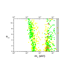
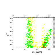
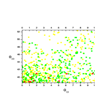
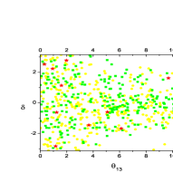
Figure 7: Constraints on some of the low energy neutrino parameters in the $SO(10)$-inspired scenario for normal ordering and $I<V_{L}<V_{CKM}$ [48]. The yellow, green and red points correspond respectively to $\alpha_{2}=5,4,1$.

7.3 Discrete flavour symmetries

An account of heavy neutrino flavour effects is important when leptogenesis is embedded within theories that try to explain tribimaximal mixing for the leptonic mixing matrix via flavour symmetries. It has been shown in particular that if the symmetry is unbroken then the $C\!P$ asymmetries of the RH neutrinos would exactly vanish since the basis of the three heavy neutrino flavours would be exactly orthonormal. On the other hand when the symmetry is broken, for the naturally expected values of the symmetry breaking parameters, then the observed matter-antimatter asymmetry can be successfully reproduced [50]. It is interesting that in a minimal picture based on a $A4$ symmetry , one has a RH neutrino mass spectrum with $10^{15}\,{\rm GeV}\gtrsim M_{3}\gtrsim M_{2}\gtrsim M_{1}\gg 10^{12}\,{\rm GeV}$. One has therefore that all the asymmetry is produced in the unflavoured regime and that the mass spectrum is only mildly hierarchical (it has actually the same kind of hierarchy of light neutrinos). At the same time the small symmetry breaking implies corresponds to quasi-orthonormality of the three lepton quantum states produced in the RH neutrino decays. Under these conditions the wash-out of the asymmetry produced by one RH neutrino species from the inverse decays of a lighter RH neutrino species is essentially negligible. The final asymmetry then receives a non negligible contribution from the decays of all three RH neutrinos species.

7.4 Supersymmetric models

Within a supersymmetric framework the final asymmetry calculated in the vanilla leptogenesis scenario undergoes minor changes [51]. However, supersymmetry introduces a conceptual important issue: the stringent lower bound on the reheat temperature, $T_{\rm RH}\gtrsim 10^{9}\,{\rm GeV}$, is typically marginally compatible with an upper bound from the avoidance of the so called gravitino problem $T_{\rm RH}\lesssim 10^{6-10}\,{\rm GeV}$, with the exact value depending on the parameters of the model [52] . It is quite remarkable that the solution of such a issue inspired an intense research activity on supersymmetric models able to reconcile minimal leptogenesis and the gravitino problem. Of course on the leptogenesis side, some of the discussed extensions beyond the vanilla scenario that relax the neutrino mass bounds also relax the $T_{\rm RH}$ lower bound. However, notice that in the $N_{2}$ dominated scenario, while the lower bound on $M_{1}$ simply disappears, there is still a lower bound on $T_{\rm RH}$ that is even more stringent, $T_{\rm RH}\gtrsim 6\times 10^{9}\,{\rm GeV}$ [31]. As mentioned already, with flavour effects one has the possibility to relax the lower bound on $T_{\rm RH}$ if a mild hierarchy in the RH neutrino masses is allowed together with a mild cancellation in the see-saw formula [22]. However for most models, such as sequential dominated models [38], this solution does not apply.

A major modification introduced by supersymmetry is that the critical value of the mass of the decaying RH neutrinos setting the transition from an unflavoured regime to a two-flavour regime and from a two-flavour regime to a three flavour regime is enhanced by a factor $\tan^{2}\beta$ [32, 53]. This has a practical relevance in the calculation of the asymmetry within supersymmetric models and it is quite interesting that leptogenesis becomes sensitive to such a relevant supersymmetric parameter.

8 A wish list for leptogenesis

In 2011 two important experimental results have been announced that, if confirmed, can be interpreted as quite important toward the possibility of a positive test of leptogenesis . The first result is the strong hint of a non-vanishing $\theta_{13}\simeq 9^{\circ}$ from T2K results first and then confirmed by many other experiments at more than $5\sigma$ standard deviations [37]. Very interestingly, such a value is sufficiently large to open realistically the possibility of a measurement of the neutrino oscillation $C\!P$ violating invariant $J_{CP}\propto\sin\theta_{13}\,\sin\delta$ during next years.

If this measurement will give a non-vanishing result, this will have some direct model independent important consequences. First of all, even the small contribution to the final asymmetry uniquely stemming from a Dirac phase could be sufficient to reproduce the observed final asymmetry [36, 22]. In any case, the presence of $C\!P$ violation at low energies would certainly support also the presence of $C\!P$ violation at high energies, since given a generic theoretical model predicting the neutrino Dirac mass matrix $m_{D}$, these are in general both present. However, there is an even more important practical relevance of such a measurement, even if in the end this will indicate a vanishing value of $J_{CP}$ within the experimental error. The reason is that such a measurement of $J_{CP}$ will provide an additional constraint in specific see-saw models able to produce simultaneous predictions on the low energy neutrino parameters and on the final asymmetry in leptogenesis. The interesting case of $SO(10)$-inspired leptogenesis offers a definite example. By plugging more and more information from low energy neutrino experiments, we will be able more and more strongly to test the models.

At the same time the hint of a $\simeq 125\,{\rm GeV}$ Higgs boson reported by the ATLAS and CMS collaborations can be also interpreted as a positive result for leptogenesis. First of all because leptogenesis relies on the Higgs mechanism and second because the measurement of the Higgs boson mass could in future open new opportunities for additional phenomenological information to be imposed on leptogenesis scenarios for example relying on the requirement of vacuum stability [55].

What are other possible future experimental developments that could be important for testing leptogenesis? An improved information from absolute neutrino mass scale experiments, both on the sum of the neutrino masses from cosmology and on $m_{ee}$ from $0\nu\beta\beta$ experiments could be crucial especially if these phenomenologies will definitively confirm the upper bound $m_{1}\lesssim 0.1\,{\rm eV}$ but at the same time will detect a positive signal $m_{1}\sim 10^{-2}\,{\rm eV}$, within the reach of future experiments in next 5-10 years. In this case the a desirable leptogenesis neutrino mass window $10^{-3}\,{\rm eV}\lesssim m_{1}\lesssim 10^{-1}\,{\rm eV}$ would be confirmed . At the same time it is likely that a measurement of the neutrino mass ordering will be possible when the information from absolute neutrino mass scale experiments is combined with neutrino oscillation experiments. Moreover, with a large $\theta_{13}\sim 9^{\circ}$ value, even just neutrino oscillation experiments could be sufficient to determine the mass ordering within next years. In this case a precise measurement of the allowed region in the plane $m_{ee}-\sum_{i}\,m_{i}$ would provide a positive test of specific leptogenesis scenarios, such as $SO(10)$-inspired leptogenesis, especially when a condition of independence of the initial conditions is imposed [54]. It is therefore quite exciting that even just the expected new information from (in most cases already data taking) low energy neutrino experiments will be able to test models of leptogenesis in a substantial way during next years. In conclusion, with leptogenesis, we have the fascinating opportunity to probe at the same time both a new stage in the early Universe history in cosmology and physics beyond the SM.

8.1 Acknowledgements

PDB acknowledges financial support from the NExT/SEPnet Institute, from the STFC Rolling Grant ST/G000557/1 and from the EU FP7 ITN INVISIBLES (Marie Curie Actions, PITN- GA-2011- 289442). I wish to thank S. Antusch, E. Bertuzzo, S. Blanchet, W. Buchmuller, F. Feruglio, D. Jones, S. King, L. Marzola, M. Plumacher, G. Raffelt, A. Riotto for a fruitful collaboration on leptogenesis. I also wish to thank Asmaa Abada, Steve Blanchet and Wilfried Buchmüller for useful comments and the Laboratoire de Physique Théorique, Université de Paris-Sud 11 (Orsay) for the warm hospitality during the completion of this work. This review is dedicated in memory of Alexey Anisimov.

References

- [1] A. D. Sakharov, Pisma Zh. Eksp. Teor. Fiz. 5 (1967) 32 [JETP Lett. 5 (1967) 24] [Sov. Phys. Usp. 34 (1991) 392] [Usp. Fiz. Nauk 161 (1991) 61].
- [2] J. H. Christenson, J. W. Cronin, V. L. Fitch and R. Turlay, Phys. Rev. Lett. 13 (1964) 138.
- [3] Y. Fukuda et al. [Super-Kamiokande Collaboration], Phys. Rev. Lett. 81 (1998) 1562 [hep-ex/9807003].
- [4] M. Fukugita and T. Yanagida, Phys. Lett. B 174, 45 (1986).
- [5] P. Minkowski, Phys. Lett. B 67, 421 (1977); M. Gell-Mann, P. Ramond and R. Slansky, Proceedings of the Supergravity Stony Brook Workshop, New York 1979, eds. P. Van Nieuwenhuizen and D. Freedman, North-Holland publisher; T. Yanagida, Proceedings of the Workshop on Unified Theories and Baryon Number in the Universe, Tsukuba, Japan 1979, ed.s A. Sawada and A. Sugamoto, KEK publisher; R. N. Mohapatra, G. Senjanovic, Phys. Rev. Lett. 44, 912 (1980).
- [6] A. G. Riess et al. [Supernova Search Team Collaboration], Observational Evidence from Supernovae for an Accelerating Universe and a Cosmological Constant, Astron. J. 116 (1998) 1009; S. Perlmutter et al. [Supernova Cosmology Project Collaboration], Astrophys. J. 517 (1999) 565 [astro-ph/9812133].
- [7] A. H. Guth, Phys. Rev. D 23 (1981) 347.
- [8] E. Komatsu et al. [WMAP], Astrophys. J. Suppl. 192 (2011) 18.
- [9] A. G. Riess et al., “A Redetermination of the Hubble Constant with the Hubble Space Telescope from a Differential Distance Ladder,” Astrophys. J. 699 (2009) 539.
- [10] R. I. Epstein, J. M. Lattimer and D. N. Schramm, Nature 263 (1976) 198.
- [11] D. Kirkman, D. Tytler, N. Suzuki, J. M. O’Meara and D. Lubin, Astrophys. J. Suppl. 149 (2003) 1 [astro-ph/0302006].
- [12] A. G. Cohen, A. De Rujula and S. L. Glashow, Astrophys. J. 495 (1998) 539 [astro-ph/9707087].
- [13] V. A. Kuzmin, V. A. Rubakov and M. E. Shaposhnikov, Phys. Lett. B 155 (1985) 36.
- [14] M. Carena, G. Nardini, M. Quiros and C. E. M. Wagner, Nucl. Phys. B 812 (2009) 243 [arXiv:0809.3760 [hep-ph]].
- [15] For a detailed review on neutrino physics see S. F. King, “Neutrino mass,” [arXiv:0712.1750 [physics.pop-ph]].
- [16] G. L. Fogli, E. Lisi, A. Marrone, A. Palazzo and A. M. Rotunno, Phys. Rev. D 84 (2011) 053007; T. Schwetz, M. Tortola, J. W. F. Valle, [arXiv:1108.1376 [hep-ph]].
- [17] C. .Kraus, B. Bornschein, L. Bornschein, J. Bonn, B. Flatt, A. Kovalik, B. Ostrick and E. W. Otten et al., Eur. Phys. J. C 40 (2005) 447; V. N. Aseev et al. [Troitsk Collaboration], Phys. Rev. D 84 (2011) 112003. E. W. Otten and C. Weinheimer, Rept. Prog. Phys. 71 (2008) 086201.
- [18] E. Andreotti et al., Astropart. Phys. 34 (2011) 822.
- [19] See for example: F. Mandl and G. Shaw, “Quantum Field Theory,” Chichester, Uk: Wiley (2010) 478 p.
- [20] J. A. Casas and A. Ibarra, Nucl. Phys. B 618 (2001) 171.
- [21] See W. Buchmuller, P. Di Bari and M. Plumacher, Annals Phys. 315 (2005) 305 and references therein.
- [22] S. Blanchet and P. Di Bari, Nucl. Phys. B 807 (2009) 155.
- [23] L. Covi, E. Roulet and F. Vissani, Phys. Lett. B 384 (1996) 169.
- [24] S. Davidson and A. Ibarra, Phys. Lett. B 535, 25 (2002).
- [25] S. Blanchet and P. Di Bari, JCAP 0606 (2006) 023.
- [26] A. Pilaftsis, Phys. Rev. D 56 (1997) 5431.
- [27] T. Hambye and G. Senjanovic, Phys. Lett. B 582 (2004) 73; S. Antusch and S. F. King, Phys. Lett. B 597 (2004) 199.
- [28] G. Lazarides and Q. Shafi, Phys. Lett. B 258 (1991) 305; T. Asaka, K. Hamaguchi, M. Kawasaki and T. Yanagida, Phys. Lett. B 464 (1999) 12; G. F. Giudice, M. Peloso, A. Riotto and I. Tkachev, JHEP 9908 (1999) 014.
- [29] See S. Blanchet, Z. Chacko, S. S. Granor, R. Mohapatra. Phys. Rev. D82 (2010) 076008 and references therein.
- [30] A. Basboll and S. Hannestad, JCAP 0701 (2007) 003; A. De Simone and A. Riotto, JCAP 0708 (2007) 002; M. Beneke, B. Garbrecht, M. Herranen and P. Schwaller, Nucl. Phys. B 838 (2010) 1; A. Anisimov, W. Buchmuller, M. Drewes, S. Mendizabal, Annals Phys. 326 (2011) 1998-2038; G. F. Giudice, A. Notari, M. Raidal, A. Riotto and A. Strumia, Nucl. Phys. B 685 (2004) 89.
- [31] P. Di Bari, Nucl. Phys. B 727 (2005) 318.
- [32] A. Abada, S. Davidson, A. Ibarra, F. X. Josse-Michaux, M. Losada and A. Riotto, JHEP 0609 (2006) 010.
- [33] E. Nardi, Y. Nir, E. Roulet and J. Racker, JHEP 0601 (2006) 164.
- [34] S. Blanchet, P. Di Bari and G. G. Raffelt, JCAP 0703 (2007) 012; A. De Simone and A. Riotto, JCAP 0702 (2007) 005; M. Beneke, B. Garbrecht, C. Fidler, M. Herranen and P. Schwaller, Nucl. Phys. B 843 (2011) 177.
- [35] S. Blanchet, P. Di Bari, D. A. Jones and L. Marzola, arXiv:1112.4528 [hep-ph].
- [36] A. Abada, S. Davidson, A. Ibarra, F. X. Josse-Michaux, M. Losada and A. Riotto, JHEP 0609 (2006) 010; S. Blanchet and P. Di Bari, JCAP 0703 (2007) 018; A. Anisimov, S. Blanchet and P. Di Bari, JCAP 0804 (2008) 033.
- [37] K. Abe et al. [T2K Collaboration], Phys. Rev. Lett. 107 (2011) 041801 [arXiv:1106.2822 [hep-ex]]; P. Adamson et al. [MINOS Collaboration], arXiv:1108.0015 [hep-ex]; Y. Abe et al. [DOUBLE-CHOOZ Collaboration], arXiv:1112.6353 [hep-ex]. F. P. An et al. [DAYA-BAY Collaboration], arXiv:1203.1669 [hep-ex]; J. K. Ahn et al. [RENO Collaboration], Phys. Rev. Lett. 108 (2012) 191802 [arXiv:1204.0626 [hep-ex]].
- [38] S. F. King, Rept. Prog. Phys. 67 (2004) 107.
- [39] O. Vives, Phys. Rev. D 73 (2006) 073006.
- [40] S. Antusch, P. Di Bari, D. A. Jones and S. F. King, arXiv:1003.5132.
- [41] R. Barbieri, P. Creminelli, A. Strumia and N. Tetradis, Nucl. Phys. B 575 (2000) 61; G. Engelhard, Y. Grossman, E. Nardi and Y. Nir, Phys. Rev. Lett. 99 (2007) 081802.
- [42] S. Antusch, P. Di Bari, D. A. Jones and S. F. King, arXiv:1107.6002 [hep-ph].
- [43] E. Bertuzzo, P. Di Bari and L. Marzola, Nucl. Phys. B 849 (2011) 521.
- [44] F. X. Josse-Michaux and A. Abada, JCAP 0710 (2007) 009 [hep-ph/0703084 [HEP-PH]].
- [45] S. Pascoli, S. T. Petcov and W. Rodejohann, Phys. Rev. D 68 (2003) 093007; B. Dutta and R. N. Mohapatra, Phys. Rev. D 68 (2003) 113008.
- [46] S. F. King, Nucl. Phys. B 576 (2000) 85; P. H. Frampton, S. L. Glashow and T. Yanagida, Phys. Lett. B 548 (2002) 119; S. F. King, Phys. Rev. D 67 (2003) 113010.
- [47] G. C. Branco, R. Gonzalez Felipe, F. R. Joaquim and M. N. Rebelo, Nucl. Phys. B 640, 202 (2002); E. K. Akhmedov, M. Frigerio and A. Y. Smirnov, JHEP 0309, 021 (2003).
- [48] P. Di Bari and A. Riotto, Phys. Lett. B 671 (2009) 462; P. Di Bari and A. Riotto, JCAP 1104 (2011) 037.
- [49] A. Abada, P. Hosteins, F. X. Josse-Michaux and S. Lavignac, Nucl. Phys. B 809 (2009) 183.
- [50] E. E. Jenkins and A. V. Manohar, Phys. Lett. B 668 (2008) 210; E. Bertuzzo, P. Di Bari, F. Feruglio and E. Nardi, JHEP 0911 (2009) 036; C. Hagedorn, E. Molinaro and S. T. Petcov, JHEP 0909 (2009) 115.
- [51] P. Di Bari, arXiv:hep-ph/0406115.
- [52] M. Y. Khlopov and A. D. Linde, Phys. Lett. B 138 (1984) 265; J. R. Ellis, J. E. Kim and D. V. Nanopoulos, Phys. Lett. B 145 (1984) 181; K. Kohri, T. Moroi and A. Yotsuyanagi, Phys. Rev. D 73 (2006) 123511.
- [53] S. Antusch, S. F. King and A. Riotto, JCAP 0611 (2006) 011.
- [54] P. Di Bari and L. Marzola, in preparation.
- [55] J. Elias-Miro, J. R. Espinosa, G. F. Giudice, G. Isidori, A. Riotto and A. Strumia, Phys. Lett. B 709 (2012) 222.