Drift instability in the motion of a fluid droplet with a chemically reactive surface driven by Marangoni flow

Abstract

We theoretically derive the amplitude equations for a self-propelled droplet driven by Marangoni flow. As advective flow driven by surface tension gradient is enhanced, the stationary state becomes unstable and the droplet starts to move. The velocity of the droplet is determined from a cubic nonlinear term in the amplitude equations. The obtained critical point and the characteristic velocity are well supported by numerical simulations.

I Introduction

Spontaneous motion or self-propulsion has been attracting attention in recent decades because of its potential application to biological problems such as cell motility BernheimGroswasser:2002 ; gucht:2005 ; Wiesner:2003 ; gerbal:2000 ; Cantat:2003 . These intensive studies have stemmed from the fact that mechanical properties of cells can be measured thanks to recent developments in visualization techniques lenz:2008a . In addition, several model experiments showing spontaneous motion have been carried out dosSantos:1995 ; Toyota:2009 ; sumino:2005 ; nagai:2005 ; Thutupalli2011 ; thakur:2006 . These systems consisted of relatively simple components such as oil droplets in the water Toyota:2009 . Nevertheless, the droplets give the impression of being alive in that they move spontaneously without being pushed or pulled, and they travel in straight lines, turn, and deform.

Motion in the absence of an external mechanical force has been discussed in terms of the Marangoni effect in which a liquid droplet is driven by a surface tension gradient Young:1959 ; levan:1981 . The non-uniform surface tension can be controlled by an field variable such as temperature and a chemical (typically surfactants) concentration darhuber:2005 . The mechanism is that the gradient induces convective flow inside and outside of a droplet, which leads to motion of the droplet itself. Similar flow and resulting motion are observed for a solid particle in phoretic phenomena such as thermophoresis anderson:1989 ; jiang:2009 . In both systems, objects are swimming in a fluid.

The velocity of the above-mentioned motion is reasonably well described using linear theories Young:1959 ; anderson:1989 ; julicher:2009 . This implies that the direction of motion is determined by some asymmetry in the system such as a temperature gradient (and/or a concentration gradient). In the case of solid, an asymmetric particle has recently been created by coating half of its surface with a different material. Using this so-called Janus particle, the motion along a gradient created by the particle itself, which is referred to as self-phoresis, was realized Paxton:2004 ; jiang:2010 ; golestanian:2010 . The asymmetric field in this case is not given externally but is created by consuming the energy supplied uniformly from outside. Nevertheless, linear theory still works sufficiently well since the particle has inherently asymmetric surface properties.

In contrast to the solid particle, fluid droplets are dynamic and their surface properties cannot be fixed due to internal diffusion. Motion in an isotropic system cannot be described using a linear approach; it requires symmetry breaking arising from a nonlinear term john:2008 . In fact, spontaneous motion has been discussed using reaction-diffusion equations, which are nonlinear partial differential equations, and is called as drift instability or drift bifurcation krischer:1994 ; schweitzer:1998 ; ohta:2009 . Despite this, there has been few attempts to consider the mechanics and hydrodynamics of spontaneous motion.

In the present work, we derive amplitude equations showing drift bifurcation from a set of equations for concentration fields taking hydrodynamics into consideration. All of the coefficients have clear physical meanings, and can in principle be measured. Our study is inspired by earlier pioneering works on the motion of reactive droplets ryazantsev:1985 ; rednikov:1989 . While these studies mainly focused on linear stability and response to an external force, our purpose is to derive equations containing nonlinear terms and obtain the characteristic velocity of a droplet.

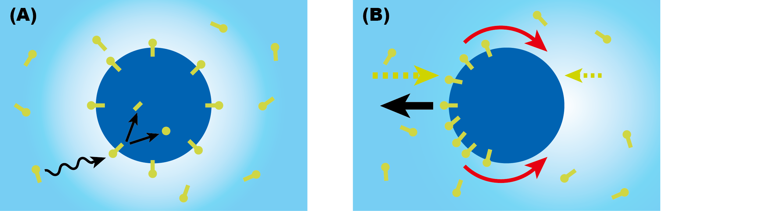
Figure 1: (Color Online) Schematic illustration of the system in this study. Surfactants dissolve in the outer fluid and some are adsorbed at the interface between the inner and the outer fluids. These surfactants reduce the surface tension of the droplet. (A) No droplet motion occurs for an isotropic distribution of surfactants. (B) When the surfactant distribution becomes asymmetric, the flow (thin red arrows) occurs and the droplet starts to move in the direction of the thick black arrow. The flux of surfactants are shown in broken arrows. The background gradation represents surfactant concentration.

II model

We consider an axisymmetric system containing a spherical droplet in a fluid which has an inner and/or outer surfactant concentration of $c(r,\theta)$, and a velocity field of ${\bf v}(r,\theta)=(v_{r}(r,\theta),v_{\theta}(r,\theta))$ in the co-moving frame with the droplet sadhal:1996 . Near the critical point of drift bifurcation, the velocity of the droplet is slow so that ${\bf v}(r,\theta)$ can be described by low-Reynolds hydrodynamics, that is, the Stokes equation

$$\eta\nabla^{2}{\bf v}=\nabla p,$$ (1)

with the incompressible condition $\nabla\cdot{\bf v}=0$. $\eta$ is the viscosity of the inner or outer fluid and $p$ is the pressure. We assume a linear relationship between the concentration of surfactants at the interface $\Gamma(\theta)$ and surface tension

$$\gamma(\theta) =\gamma_{0}+\gamma_{c}\Gamma(\theta)$$ (2)

using the surface tension $\gamma_{0}$ without surfactants. The surfactant concentration at the interface can be expanded using Legendre polynomials as

$$\Gamma(\theta,t) =\sum_{n=0}^{\infty}A_{n}(t)P_{n}(\cos\theta).$$ (3)

Here we restrict our attention to non-deformable droplets. We consider only the $n=0$ and $n=1$ modes, and neglect the higher modes. The solution of the Stokes equation for Marangoni flow for a given surface tension with an arbitrary distribution has been derived levan:1981 ; Kitahata:2011 . It can be seen that the velocity of a droplet is proportional to the first mode as

$$u=u_{1}A_{1},$$ (4)

where

$$u_{1} =-\frac{2\gamma_{c}}{3(3\eta_{i}+2\eta_{o})},$$ (5)

and the subscripts “i” and “o” denote the inner and outer fluid, respectively. $\gamma_{c}$ is the strength of surface activity. Since the surface tension is typically smaller for higher concentrations of surfactants at the interface, $\gamma_{c}$ is negative and accordingly $u_{1}>0$. $u_{1}$ determines the strength of the chemomechanical coupling; the flow field is sensitive to the anisotropy when $|u_{1}|$ is large. Stronger coupling can be found for surfactants with higher surface activity.

The concentration of molecules adsorbed at the interface is in balance with the bulk concentration field near the interface due to the adsorption-desorption equilibrium as

$$\alpha\Gamma(\theta)=c(R,\theta),$$ (6)

where $\alpha$ is interpreted as the inverse of Henry’s constant $K_{\rm H}$ for adsorption equilibrium and has the dimensions of inverse length chang:1995 . For a low surfactant concentration at the interface, $\alpha$ is simply described as $k_{d}/k_{a}$ where $k_{a}$ and $k_{d}$ are the adsorption rate from bulk and desorption rate from surface, respectively. For this reason, $\alpha$ is not dimensionless but has the dimension of length. For surfactants with higher surface activity $\alpha$ can be small, for instance, $\alpha\simeq 10^{-1}$ m^-1 chang:1995 . The concentration of surfactants at the interface can be expressed assadhal:1996

$$\frac{\partial\Gamma}{\partial t}+v_{\theta}(R)\nabla_{s}\Gamma=D_{s}\nabla_{s}^{2}\Gamma-\kappa_{s}\Gamma+\left[D_{o}\frac{\partial c}{\partial r}-D_{i}\frac{\partial c}{\partial r}\right]_{r=R},$$ (7)

where the surface derivative is defined as $\nabla_{s}=(1/R)\partial/\partial\theta$ for a sphere. $D$ ($D_{i}$ and $D_{o}$) and $D_{s}$ are the bulk and surface diffusion constants, respectively. The surfactants are reactive; molecules dissolved in the bulk are adsorbed onto the interface, and after a characteristic time $\kappa_{s}^{-1}$ they lose their surfactant functionality, for instance by decomposing into a head and a tail (see Fig.1). We describe this by a linear reaction $-\kappa_{s}\Gamma$ with a consumption rate $\kappa_{s}$. In this model, we implicitly assume addition and removal of surfactants at the interface, which depend on the divergence of the two-dimensional velocity fields.

We derive the amplitude equation near the onset of drift instability where $A_{1}\sim\epsilon$ is small so that $u\sim\epsilon$. Our goal is to obtain the equation for the first mode

$$m\frac{dA_{1}}{dt}=gA_{1}+\epsilon\mathcal{F}_{1}(A_{1})+\epsilon^{2}\mathcal{F}_{2}(A_{1})+\cdots,$$ (8)

with coefficients $m$ and $g$, and some functions $\mathcal{F}_{1}$, $\mathcal{F}_{2},\cdots$. Taking (4) into consideration, this is equivalent to a Landau-type equation for the droplet velocity

$$\tilde{m}{du}/{dt}=\tilde{g}u+\epsilon\tilde{\mathcal{F}}_{1}(u)+\epsilon^{2}\tilde{\mathcal{F}}_{2}(u)+\cdots.$$ (9)

The basic idea is to eliminate the velocity and bulk concentration fields in order to obtain a closed form of the equations for $A_{1}$.

We hereafter focus only on the surfactant concentration in the outer fluid and therefore drop the subscript “o”. The two fluids under consideration could, for example, be water and oil, and the surfactants preferentially dissolve in either one or the other. The bulk concentration can be expressed using the Helmholtz equation with advection,

$$\frac{\partial c}{\partial t}+{\bf v}\cdot\nabla c=D\nabla^{2}c-\kappa(c-c_{\infty}).$$ (10)

The model takes into account the supply of surfactants to the bulk in order to maintain a constant concentration $c_{\infty}$ far from the interface. The time scale is given by $\kappa$. We expand (10) around the critical point of drift instability; the velocity of the droplet, $u$, or the Péclet number $Ru/D$ is set as a small parameter $\epsilon$. We can solve this equation perturbatively as

$$c(r,\theta)=c_{\infty}+c^{(0)}(r,\theta)+\epsilon c^{(1)}(r,\theta)+\cdots$$ (11)

with the boundary conditions at infinity $c(\infty,\theta)=c_{\infty}$ and at the interface (see (6)). For the orders of $\epsilon^{0}$ and $\epsilon$ , (10) is expressed as

$$\frac{dc^{(0)}}{dt} =D\nabla^{2}c^{(0)}-\kappa c^{(0)},$$ (12)

$$\frac{dc^{(1)}}{dt}+{\bf v}\cdot\nabla c^{(0)} =D\nabla^{2}c^{(1)}-\kappa c^{(1)}.$$ (13)

The resulting $c(r)$ is then substituted back into (7). Due to the boundary condition (6), the solution of $c(r,\theta)$ contains the individual modes $A_{n}$ and coupled modes $A_{n}A_{m}$. The nonlinear time evolution equations of $A_{n}$ are then obtained (see (16) and (17)).

II.1 uniform distribution

We assume that the relaxation of the bulk concentration field is fast. The zeroth order solution of (12) is then

$$c^{(0)}(r,t)=\left(\alpha A_{0}(t)-c_{\infty}\right)\frac{k_{0}(r/\lambda)}{k_{0}(R/\lambda)},$$ (14)

where $k_{n}(x)$ is an $n$th-order modified spherical Bessel function of the second kind arfken:1968 . The result is plotted in Fig.2(A). A steep gradient can be observed in the typical length scale $\lambda=\sqrt{D/\kappa}$. The gradient is sustained by surface reaction characterized by $\kappa_{s}$ in (7). For $R\gg\lambda$, the surface concentration is given by

$$A_{0} \simeq\frac{c_{\infty}}{\kappa_{s}\lambda/D+\alpha},$$ (15)

leading to a gap $c_{\infty}-\alpha A_{0}$ between the concentration near the surface and at infinity. Since this gap is proportional to $\kappa_{s}$, the concentration gradient is driven by surface reactions.

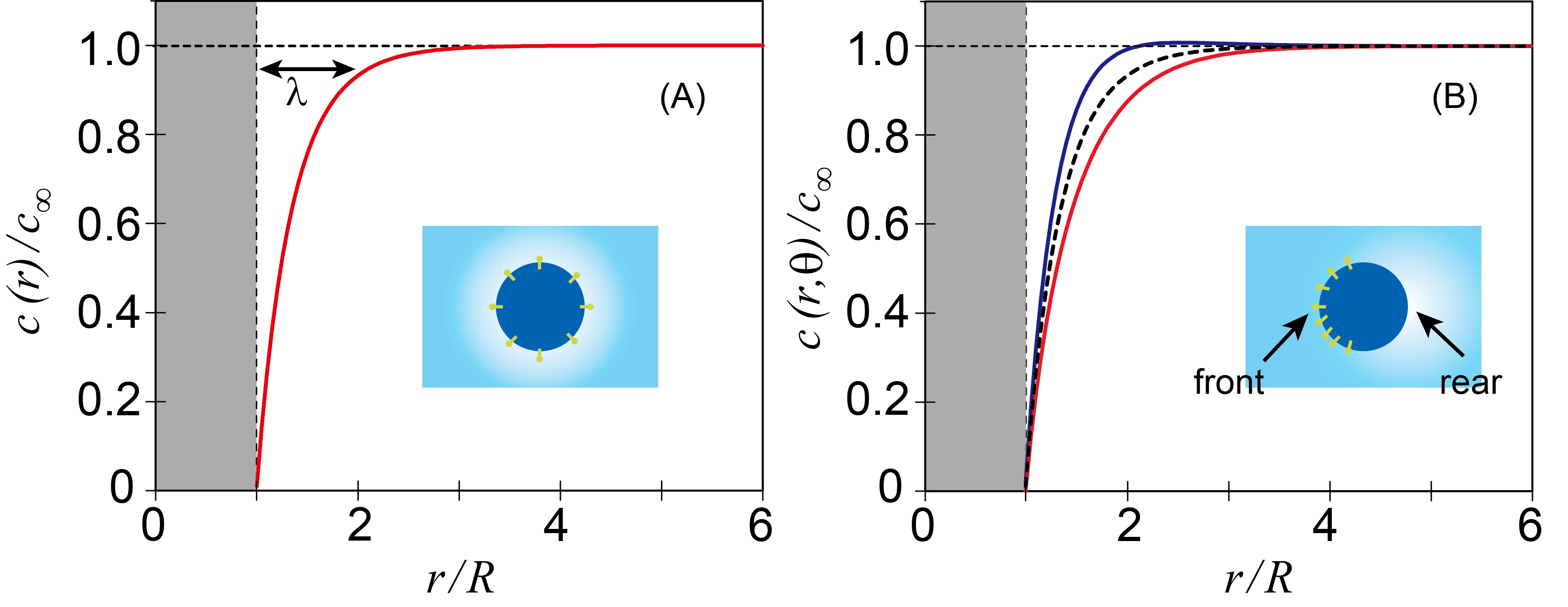
Figure 2: (Color Online) Distribution of bulk concentration field. (A) Isotropic distribution when $\lambda=0.5$, $\alpha=0.01$, and $u_{1}/D=0$. (B) Anisotropic distribution with $u_{1}/D=2.0$. The blue (dark grey) line shows $c(r,\theta=0)$ (front) and the red (light grey) line shows $c(r,\theta=\pi)$ (rear). The uniform distribution of (A) is shown in (B) as a dashed line.

II.2 Amplitude equations

A weakly nonlinear analysis up to the order of $\epsilon^{3}$ shows

$$\frac{dA_{0}}{dt}= -\kappa_{s}A_{0}+\frac{\lambda+R}{\lambda R}D(c_{\infty}-\alpha A_{0})+\Lambda^{(2)}_{0}A_{1}^{2},$$ (16)

$$\frac{dA_{1}}{dt}= -\Lambda^{(1)}_{1}\left(1-\frac{u_{1}}{u_{1}^{*}}\right)A_{1}-\Lambda^{(3)}_{1}A_{1}^{3},$$ (17)

where the coefficients are

$$\Lambda^{(2)}_{0} =\Lambda_{02}u_{1}\alpha+\Lambda_{03}\frac{u_{1}^{2}}{D}(c_{\infty}-\alpha A_{0})-\frac{3u_{1}}{2R},$$ (18)

$$\Lambda^{(1)}_{1} =\frac{2D_{s}}{R^{2}}+\kappa_{s}+\frac{D\alpha}{\lambda},$$ (19)

$$\Lambda^{(3)}_{1} =\Lambda_{13}\frac{\alpha u_{1}^{2}}{D}+\Lambda_{14}\frac{u_{1}^{3}}{D^{2}}(c_{\infty}-\alpha A_{0}),$$ (20)

with the coefficients $\Lambda_{ab}$ being dependent only on $\lambda$ and $R$. The explicit forms of $\Lambda_{ab}$ are shown in the Appendix (see (74)-(78)). The critical point of the drift bifurcation occurs when the first term on the right-hand side of (17) changes its sign;

$$u_{1}^{*} =\frac{\frac{2D_{s}}{R^{2}}+\kappa_{s}+\frac{D\alpha}{\lambda}}{\Lambda_{12}(c_{\infty}-\alpha A_{0})}.$$ (21)

For $u_{1}\leq u_{1}^{*}$, a stationary state is stable whereas it becomes destabilized and the droplet moves for $u_{1}>u_{1}^{*}$. For $\alpha\ll\kappa_{s}\lambda/D$, the steady-state velocity of the droplet is given by

$$u\simeq u_{0}\sqrt{1-\frac{u_{1}^{*}}{u_{1}}},$$ (22)

where the characteristic velocity is $u_{0}=\sqrt{D\kappa R/\lambda}$ for $R\gg\lambda\gtrsim 0.01R$.

The instability can be explained as follows. First, small fluctuations in the surfactant concentration at the interface give rise to a small $A_{1}$, which induces convective flow around the droplet. The flow then distorts the bulk concentration field through the advection term. Above the critical point, the distortion overcomes the relaxation due to diffusion and amplifies the first mode $A_{1}$ leading to further flow and motion of the droplet. In fact, Fig. 2(B) shows that the gradient in the bulk concentration at the front of the droplet (relative to the direction of motion) is steeper than that at the rear. This steeper gradient causes a larger flux from the bulk to the surface, and thus leads to an inhomogeneous surface concentration. Above the critical point, the velocity increases with $u_{1}$ as in Fig.3. In actual experiments, the size of a droplet may be the suitable parameter to vary. We find that there is an optimal droplet size for producing the highest velocity (Fig.3B). The two critical radii $R^{*}_{1}\simeq D_{s}/c_{\infty}u_{1}\lambda$ and $R^{*}_{2}\simeq c_{\infty}u_{1}\lambda^{2}/(\lambda\kappa_{s}+D\alpha)$ arise from two stabilizing factors: surface diffusion and surface reaction. Both of them are balanced with the effect of advection. The size range for efficient self-propulsion increases with $u_{1}$. The time evolution of the first mode below the critical point can be expressed as $A_{1}\sim e^{-t/\tau_{\rm relax}},$where the relaxation time is

$$\tau_{\rm relax} =\left[\frac{2D_{s}}{R^{2}}+\kappa_{s}+\frac{D\alpha}{\lambda}\right]^{-1}\left(1-\frac{u_{1}}{u_{1}^{*}}\right)^{-1},$$ (23)

which diverges at $u_{1}=u_{1}^{*}$.

In the linear term of (17), $\Lambda_{1}^{(1)}/u_{1}^{*}=\Lambda_{12}(c_{\infty}-\alpha A_{0})$, which corresponds to (50) with (76), destabilizes the stationary state. The physical origin of the destabilization is motion of the droplet. This can be seen in the first bracket in the velocity in radial direction (29), which leads to the destabilization term. The first term in the bracket $-uP_{1}(\cos\theta)$ corresponds to translational motion of the droplet in the co-moving frame while the second term $u(R/r)^{3}P_{1}(\cos\theta)$ arises from convective flow around the droplet. We investigated the contributions from both terms separately, and found that two terms have opposite effects; the first term (translational motion) destabilizes the stationary state while the latter (convection) stabilizes the instability. The instability is realized because the former always has stronger effect.

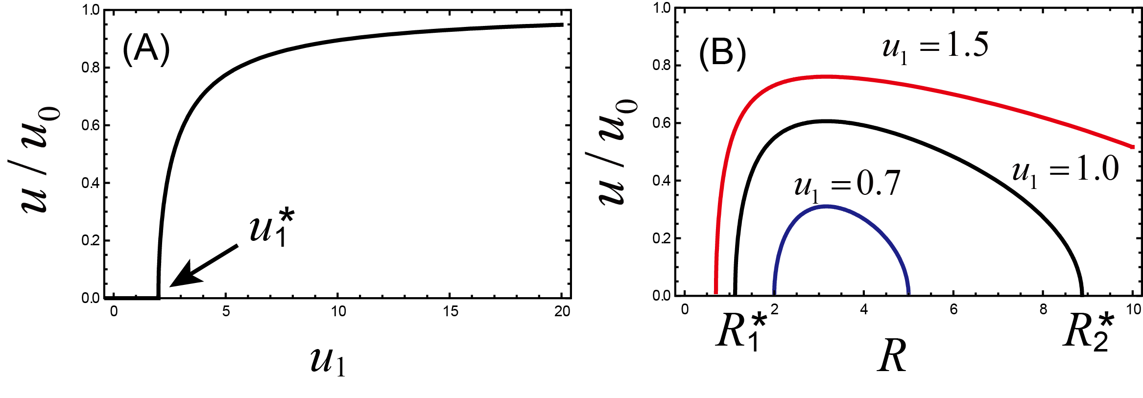
Figure 3: (Color Online) Bifurcation diagram for spontaneous motion. The bifurcation parameters are chosen to be $u_{1}$ (A) and $R$ (B).

III Numerical simulations

Numerical simulations are performed using spherical coordinates for an axisymmetric three-dimensional system. Both the radial and angular directions are discretized with $N+1$ mesh points. It is convenient to use the non-dimensionalized form of equations (7) and (10).

$$\frac{\partial\tilde{\Gamma}}{\partial\tilde{t}}+\frac{\tilde{v}_{\theta}(\tilde{R},\theta)}{\tau}\tilde{\nabla}_{s}\tilde{\Gamma} =l^{2}_{s}\tilde{\nabla}_{s}^{2}\tilde{\Gamma}-\tilde{\Gamma}+\frac{\partial\tilde{c}}{\partial\tilde{r}},$$ (24)

$$\tau\frac{\partial\tilde{c}}{\partial\tilde{t}}+\tilde{{\bf v}}\cdot\tilde{\nabla}\tilde{c} =l^{2}\tilde{\nabla}^{2}\tilde{c}-\tilde{c},$$ (25)

where $\tilde{\Gamma}=(R\kappa_{s}/Dc_{\infty})\Gamma,$ $\tilde{c}=(c-c_{\infty})/c_{\infty},$ $\tilde{{\bf v}}={\bf v}/\kappa R$, $\tilde{t}=\kappa_{s}t,$ $\tilde{r}=r/R,$ $\tau=\kappa_{s}/\kappa,$ $l_{s}=\sqrt{D_{s}/\kappa_{s}R^{2}},$ and $l=\sqrt{D/\kappa R^{2}}$. The velocity field is also non-dimensionalized as $\tilde{u}=\tilde{u}_{1}\tilde{A}_{1},$ where $\tilde{u}_{1}=(Dc_{\infty}/\kappa\kappa_{s}R^{2})u_{1},$ and $\tilde{A}_{n}=(R\kappa_{s}/Dc_{\infty})A_{n}.$ The boundary condition is rewritten as $\tilde{\alpha}\tilde{\Gamma}=\tilde{c}(1)+1$ with $\tilde{\alpha}=(D/\kappa_{s}R)\alpha$. We choose $\tilde{u}_{1}$ to be a bifurcation parameter, which induces instability above a certain threshold. $\tau$ is assigned a small value of 0.04. We estimate the critical point from the relaxation time using (23).

We estimate the critical point from the relaxation time above the transition with (23). Since the time evolution of $A_{1}$ decays exponentially, we estimate the relaxation time by fitting the semi-log plot of $A_{1}$ as a function of time. From the $x$-intercept of the plot of relaxation time as a function of $u_{1}$, we obtain the value of $u_{1}$ at the critical point. The critical point weakly depends on the number of mesh points; for instance, for $\tilde{l}=0.2$ and $\tilde{l}_{s}=1.0$, our theory predicts $\tilde{u}^{*}_{1}=1.03$ while the numerical results show $\tilde{u}^{*}_{1}=1.09$ for $N=100$. As the mesh number is increased, the estimated critical point becomes closer to the predicted value $\tilde{u}_{1}^{*}=1.08$ for $N=200$ and $\tilde{u}_{1}^{*}=1.04$ for $N=400$. Nevertheless, Fig. 4 shows that the normalized plot using numerically estimated values does not depend on the number of mesh points. We have mainly used $N=100$ for saving computational time and for earning data points.

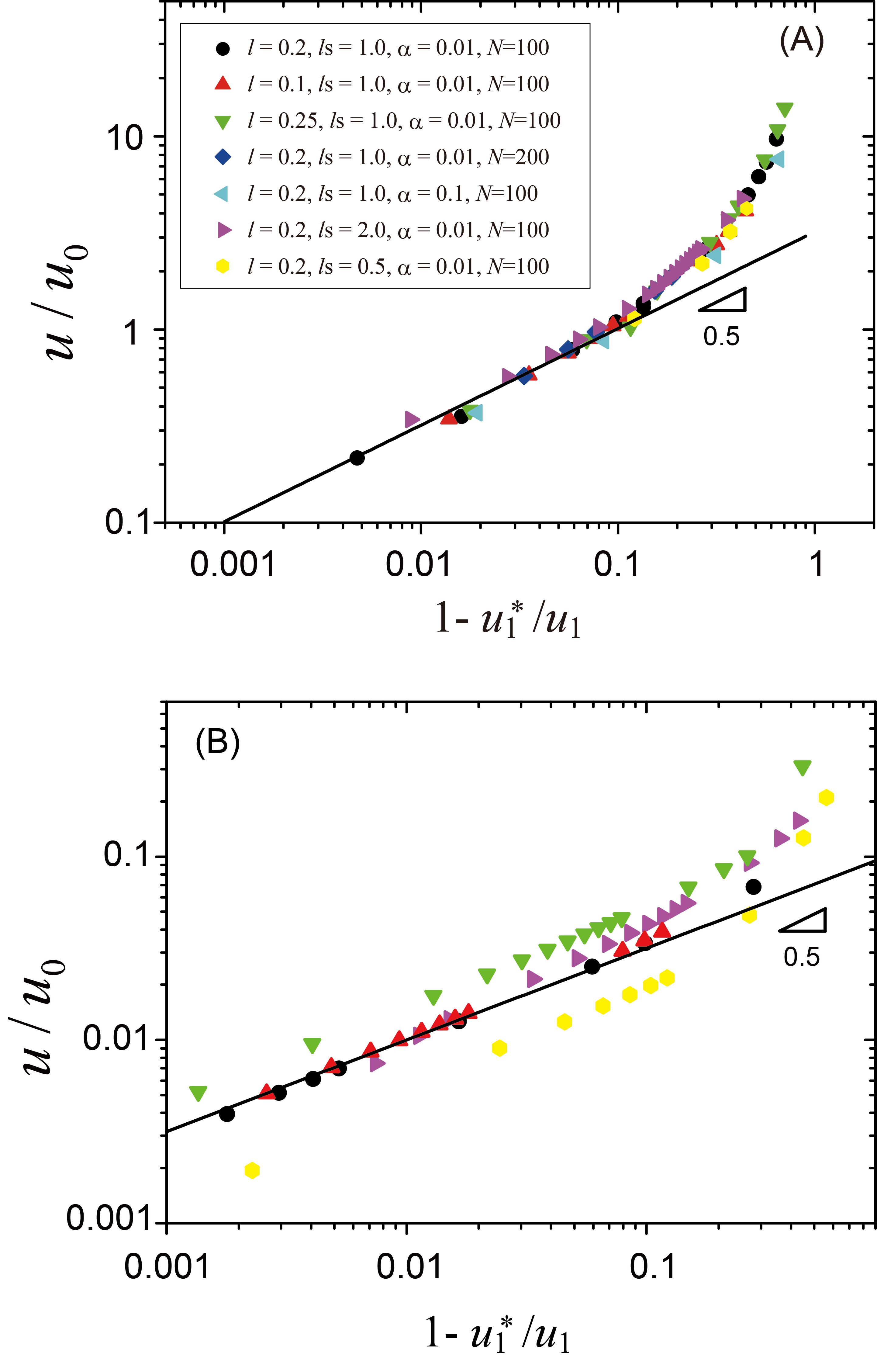
Figure 4: (Color Online) Normalized velocity of a droplet without (A) and with (B) surface advection in (24). The slope of the line is 0.5.

The numerical results show the concentration distribution around a droplet moving in the left direction . It can be seen that the concentration distribution around the droplet is asymmetric. The droplet is stationary for small $u_{1}$ whereas it moves when $u_{1}$ becomes larger. Note that the direction of motion is determined by an initially introduced small noise, and is therefore random. The velocity normalized by $u_{0}$ is plotted against the distance from the critical point in Fig. 4. Near the critical point the slope has a value of 0.5, which is comparable to the analytical result (22). A bifurcation is observed both with and without the surface advection term in (7). The characteristic velocities deviate slightly from the analytical results for some choices of parameters when the surface advection is included. This may be due to the effects of higher modes. Without the surface advection, all of the data points lie on the same curve irrespective of the parameters used.

IV Summary and Remarks

In summary, we derive amplitude equations for drift instability of a droplet driven by Marangoni flow. The critical point and the droplet velocity are calculated analytically, and good agreement is found with the results of numerical calculations. Our system is out of equilibrium due to the reaction at the interface by which the supplied energy is consumed (see (7)). This reaction maintains a concentration gradient in the radial direction. An additional key factor is the nonlinear advection term in the bulk concentration field, which leads to coupling between modes and breaks the symmetry of the system. The concentration gradient in the radial direction as well as the flux of surfactants onto the interface then becomes asymmetric. This leads to a surface tension gradient which results in motion. By contrast, surface advection is not essential for motility. Despite the linear nature of the velocity fields associated with the Stokes equation, we show that the addition of a nonlinear term in the concentration field can lead to steady motion in an isotropic system. Further studies are required in order to clarify the kinds of nonlinear effects that are necessary for motility.

Our model does not necessarily require the presence of surfactants. For instance, a uniformly heated droplet or a droplet with a source of chemicals can be tractable as the same manner with appropriate limits: $\alpha\rightarrow 1$, $D_{s}\rightarrow 0$, and $\kappa_{s}\gg 1$. In this situation, (7) is equivalent to a boundary condition for flux in the concentration field $\left[D_{o}{\bf n}\cdot\nabla c-D_{i}{\bf n}\cdot\nabla c\right]_{r=R}-\kappa_{s}c(R)=0,$ where the first and second terms represent the flux from outside and inside of the droplet, respectively. Here, the surface concentration $\Gamma$ independent of $c(r)$ does not exist. However, it is convenient to introduce a virtual surface concentration because velocity fields are essentially created by the concentrations at the surface (see (4)). It should also be stressed that similar results can be obtained using a phase-field model without explicitly considering a surface Yabunaka:2012 .

Although we focus on an outer fluid, generalization of the models to include the inner concentration is straightforward. We may also consider production rather than consumption of surfactants at an interface, in which case spontaneous motion is realized for $\gamma_{c}<0$. In fact, spontaneous motion has been observed for complexes of surfactants and ions that exhibit lower surface activity than the surfactants alone Thutupalli2011 .

Appendix A derivation of Eqs.(18)-(20)

In this appendix, we give a detailed derivation of the coefficients $\Lambda_{ab}$ in the amplitude equations (11) and (12). The dimensional analysis show that the coefficients have the dimension of length; they are functions of $\lambda$ and $R$. Introducing length and time scales, $L$ and $\tau$, the parameters are scaled as $D\sim L^{2}/\tau$, $\alpha\sim 1/L$, $A_{1}\sim 1/L^{2}$, $u=u_{1}A_{1}\sim L/\tau$, and $u_{1}\sim L^{3}/\tau$ . Then the coefficients of amplitude equations are expressed as $\Lambda_{02}\sim L^{0}$, $\Lambda_{03}\sim L$, $\Lambda_{11}\sim 1/L$, $\Lambda_{12}\sim L^{0}$, $\Lambda_{13}\sim L$, and $\Lambda_{14}\sim L^{2}$ . Using the coefficients, the steady velocity of a droplet is obtained from (12) as

$$u=u_{1}A_{1}=\sqrt{\frac{-\left(\frac{D_{s}}{R^{2}}+\kappa_{s}+\frac{D\alpha}{\lambda}\right)+\Lambda_{12}u_{1}(c_{\infty}-\alpha A_{0})}{\Lambda_{13}\frac{\alpha}{D}+\Lambda_{14}\frac{u_{1}}{D^{2}}(c_{\infty}-\alpha A_{0})}}.$$ (26)

Later, we will find $\Lambda_{12}\simeq\lambda/R$ and $\Lambda_{14}\simeq\lambda^{4}/R^{2}$ which leads to the characteristic droplet velocity under $\alpha\ll\kappa_{s}\lambda/D$ as

$$u\simeq u_{0}=\sqrt{\frac{D\kappa R}{\lambda}}.$$ (27)

In order to obtain the concrete form of the coefficients, the Helmholtz equation with nonlinear advection is solved neglecting time derivative in (6),

$$\nabla^{2}c-\frac{1}{\lambda^{2}}(c-c_{\infty}) =\frac{{\bf v}\cdot\nabla c}{D},$$ (28)

where the velocity field in the co-moving frame with the droplet is given explicitly here as levan:1981 ; Kitahata:2011

$$v^{o}_{r}(r,\theta) =-u\left(1-\frac{R^{3}}{r^{3}}\right)P_{1}(\cos\theta)$$

$$-\sum_{n=2}^{\infty}\frac{n(n+1)}{2n+1}u_{n}A_{n}\left[\left(\frac{R}{r}\right)^{n}-\left(\frac{R}{r}\right)^{n+2}\right]P_{n}(\cos\theta),$$ (29)

$$v^{o}_{\theta}(r,\theta) =-u\left(1+\frac{R^{3}}{2r^{3}}\right)\frac{dP_{1}}{d\theta}(\cos\theta)$$

$$-\sum_{n=2}^{\infty}\frac{u_{n}A_{n}}{2n+1}\left[\frac{(n-2)R^{n}}{r^{n}}-\frac{nR^{n+2}}{r^{n+2}}\right]\frac{dP_{n}(\cos\theta)}{d\theta},$$ (30)

$$v^{i}_{r}(r,\theta) =-\frac{3}{2}u\left[\left(\frac{r}{R}\right)^{2}-1\right]\cos\theta$$

$$-\sum_{n=2}^{\infty}\frac{n(n+1)}{2n+1}u_{n}A_{n}\left[\left(\frac{r}{R}\right)^{n+1}-\left(\frac{r}{R}\right)^{n-1}\right]P_{n}(\cos\theta),$$ (31)

$$v^{i}_{\theta}(r,\theta)$$

$$=-\frac{3}{2}u\left[2\left(\frac{r}{R}\right)^{2}-1\right]\frac{dP_{1}}{d\theta}$$

$$-\sum_{n=2}^{\infty}\frac{u_{n}A_{n}}{2n+1}\left[(n+3)\left(\frac{r}{R}\right)^{n+1}-(n+1)\left(\frac{r}{R}\right)^{n-1}\right]\frac{dP_{n}(\cos\theta)}{d\theta},$$ (32)

where $P_{n}(\cos\theta)$ is the $n$th-degree Legendre polynomial and

$$u_{n}=-\frac{\gamma_{c}}{2(\eta_{i}+\eta_{o})}.$$ (33)

Near the critical point of drift bifurcation, the velocity of the droplet is small and accordingly the advection term is small. The solution is expanded perturbatively as $c=c_{\infty}+c^{(0)}+c^{(1)}+c^{(2)}+\cdots$ and at each order (28) becomes

$$D_{o}\nabla^{2}c^{(0)}-\kappa_{o}c^{(0)} =0$$ (34)

,

$$D_{o}\nabla^{2}c^{(1)}-\kappa_{o}c^{(1)} =\frac{{\bf v}^{o}\cdot\nabla c^{(0)}}{D},$$ (35)

$$D_{o}\nabla^{2}c^{(2)}-\kappa_{o}c^{(2)} =\frac{{\bf v}^{o}\cdot\nabla c^{(1)}}{D}$$ (36)

for the order of $\epsilon^{2}$, and so on. Note that although we focus only on the outer concentration field, the inner concentration field yields essentially the same equations. Hereafter, we drop the subscript “o”.

The solution of the zeroth-order equation (34) satisfying the boundary condition (3) is given in (9) using $n$th-order modified spherical Bessel function of the second kind $k_{n}(x)=\sqrt{2/(\pi x)}\mathcal{K}_{n+1/2}(x)$ where $\mathcal{K}_{n}(x)$ is the $n$th-order modified Bessel function of second kind arfken:1968 . At the first order in the expansion, we will solve

$$\nabla^{2}c^{(1)}-\frac{1}{\lambda^{2}}c^{(1)}=-\frac{u_{1}A_{1}}{D}\left(1-\frac{R^{3}}{r^{3}}\right)\frac{\partial c^{(0)}}{\partial r}P_{1}(\cos\theta).$$ (37)

This equation is the form of the inhomogeneous Helmholtz equation:

$$\nabla^{2}\psi-\frac{1}{\lambda^{2}}\psi=-f(r,\theta),$$ (38)

which corresponds to $\psi=c^{(l)}$ and $f=f^{(l)}$ using $l$-th order expansion in (35) and (36). The inhomogeneous term is expanded as

$$f^{(l)}(r,\theta)=\sum_{n=0}^{\infty}f^{(l)}_{n}(r)P_{n}(\cos\theta).$$ (39)

The general solution yieldsacrivos:1962

$$\psi(r,\theta)=\sum_{n=0}^{\infty}\psi_{n}k_{n}(r/\lambda)P_{n}(\cos\theta)+\int G({\bf r,r^{\prime}})f(r,\theta)d^{3}{\bf r},$$ (40)

where the Green’s function satisfiesarfken:1968

$$\left(\nabla^{2}-\frac{1}{\lambda^{2}}\right)G({\bf r},{\bf r}^{\prime})=-\delta({\bf r}-{\bf r}^{\prime}).$$ (41)

For the Helmholtz equation in three dimensions, the Green’s function is given as

$$G({\bf r,r^{\prime}})=\frac{e^{-|{\bf r-r^{\prime}}|/\lambda}}{4\pi|{\bf r-r^{\prime}}|}.$$ (42)

The inhomogeneous term $f^{(1)}$ at the first order in expansion (37) is expressed as

$$f^{(1)}_{1}(r)=\frac{e^{-(r-R)/\lambda}}{r^{2}}R\left(1-\frac{R^{3}}{r^{3}}\right)\frac{r+\lambda}{\lambda}A_{1}(c_{\infty}-\alpha A_{0})\frac{u_{1}}{D},$$ (43)

and $f^{(1)}_{n}=0$ for $n\neq 1$. The boundary condition (3) is given as

$$c^{(1)}(R,\theta)=\alpha A_{1}P_{1}(\cos\theta).$$ (44)

The solution would be

$$c^{(1)}(r,\theta)= \left[\alpha A_{1}-\mathcal{R}_{1}(R)\right]\frac{k_{1}(r/\lambda)}{k_{1}(R/\lambda)}P_{1}(\cos\theta)$$

$$+\mathcal{R}_{1}(r)P_{1}(\cos\theta).$$ (45)

where $\mathcal{R}_{1}(r)$ is

$$\mathcal{R}^{(1)}(r)= \frac{1}{\lambda}\left[k_{1}(r/\lambda)\int_{R}^{r}f_{1}(r^{\prime})i_{1}(r^{\prime}/\lambda)r^{\prime 2}dr^{\prime}\right.$$

$$\left.+i_{1}(r/\lambda)\int_{r}^{\infty}f_{1}(r^{\prime})k_{1}(r^{\prime}/\lambda)r^{\prime 2}dr^{\prime}\right].$$ (46)

$i_{n}(x)$ is the $n$th-order modified spherical Bessel function of first kind $i_{n}(x)=\sqrt{\pi/(2x)}\mathcal{I}_{n+1/2}(x)$ using the $n$th-order modified Bessel function of first kind $\mathcal{I}_{n}(x)$. This function has a simple form

$$\mathcal{R}^{(1)}(R)=\frac{1}{\lambda}i_{1}(R/\lambda)\int_{R}^{\infty}f_{1}(r^{\prime})k_{1}(r^{\prime}/\lambda)r^{\prime 2}dr^{\prime}.$$ (47)

The flux is expressed as

$$\frac{\partial c^{(1)}(R)}{\partial r}= \frac{\alpha A_{1}}{\lambda}\frac{k^{\prime}_{1}(r/\lambda)}{k_{1}(R/\lambda)}P_{1}(\cos\theta)$$

$$+\left[\frac{i^{\prime}_{1}(R/\lambda)}{i_{1}(R/\lambda)}-\frac{k^{\prime}_{1}(R/\lambda)}{k_{1}(R/\lambda)}\right]\frac{\mathcal{R}^{(1)}(R)}{\lambda}P_{1}(\cos\theta).$$ (48)

For $R\gg\lambda$ (47) becomes

$$\mathcal{R}^{(1)}(R)\simeq\frac{3}{8}\frac{\lambda^{2}}{R}A_{1}(c_{\infty}-\alpha A_{0})\frac{u_{1}}{D},$$ (49)

and we obtain the flux as

$$D\frac{\partial c^{(1)}(R)}{\partial r}\simeq\left[-\frac{\alpha D}{\lambda}+\frac{3}{4}\frac{\lambda}{R}(c_{\infty}-\alpha A_{0})u_{1}\right]A_{1}P_{1}(\cos\theta).$$ (50)

The concrete form of $\mathcal{R}^{(1)}(r)$ is

$$\mathcal{R}^{(1)}(r) =\frac{u_{1}A_{1}e^{-(r-R)/\lambda}}{8Dr^{3}}\left[2(r-R)^{2}R(2r+R)\right.$$

$$\left.+6r(r-R)R\lambda-3r(r-2R)\lambda^{2}-3r\lambda^{3}\right](c_{\infty}-\alpha A_{0}),$$ (51)

and the concentration is

$$c^{(1)}(r,\theta) =\frac{A_{1}Re^{-(r-R)/\lambda}}{4r^{3}(R+\lambda)}\left[4R\alpha r(r+\lambda)\right.$$

$$\left.+\frac{u_{1}}{D}\left(-3r^{2}R^{2}-3rR^{2}\lambda+2r^{3}(R+\lambda)+R^{3}(R+\lambda)\right)\right.$$

$$\left.\times(c_{\infty}-\alpha A_{0})\right]P_{1}(\cos\theta),$$ (52)

which is shown in Fig.2(B). Note that without the assumption of $R\gg\lambda$ the second term inside the bracket of (50) is replaced by $\frac{3R\lambda}{4(R+\lambda)^{2}}(c_{\infty}-\alpha A_{0})u_{1}$, which is always positive. This implies that this term destabilizes the stationary state irrespective of the value of $\lambda$, that is, $\kappa$.

Calculation of the higher order terms is tedious but straightforward. The second order term in bulk concentration field satisfies

$$\left(\nabla^{2}-\frac{1}{\lambda^{2}}\right)c^{(2)}(r,\theta)=-f^{(2)}(r,\theta),$$ (53)

where

$$f^{(2)}(r,\theta)= \frac{u_{1}A_{1}}{D}\left(1-\frac{R^{3}}{r^{3}}\right)\frac{\partial c^{(1)}}{\partial r}P_{1}$$

$$+\frac{u_{1}A_{1}}{D}\left(1+\frac{R^{3}}{2r^{3}}\right)\frac{1}{r}\frac{\partial c^{(1)}}{\partial\theta}\frac{dP_{1}}{d\theta}.$$ (54)

This is decomposed as

$$f^{(2)}(r,\theta)=f^{(2)}_{0}(r)P_{0}(\cos\theta)+f^{(2)}_{2}(r)P_{2}(\cos\theta)$$ (55)

using

$$P_{1}(\cos\theta)P_{1}(\cos\theta)=\frac{1}{3}P_{0}(\cos\theta)+\frac{2}{3}P_{2}(\cos\theta),$$ (56)

$$\frac{dP_{1}(\cos\theta)}{d\theta}\frac{dP_{1}(\cos\theta)}{d\theta}=\frac{2}{3}P_{0}(\cos\theta)-\frac{2}{3}P_{2}(\cos\theta).$$ (57)

Since we focus on the zeroth and first modes and the boundary condition is

$$c^{(2)}(R)=0,$$ (58)

the general solution is expressed as

$$c^{(2)}(r,\theta)= -\mathcal{R}^{(2)}(R)\frac{k_{0}(r/\lambda)}{k_{0}(R/\lambda)}+\mathcal{R}^{(2)}(r),$$ (59)

where

$$\mathcal{R}^{(2)}(r) =\frac{1}{\lambda}\left[k_{0}(r/\lambda)\int_{R}^{r}f^{(2)}_{0}(r^{\prime})i_{0}(r^{\prime}/\lambda)r^{\prime 2}dr^{\prime}\right.$$

$$\left.+i_{0}(r/\lambda)\int_{r}^{\infty}f^{(2)}_{0}(r^{\prime})k_{0}(r^{\prime}/\lambda)r^{\prime 2}dr^{\prime}\right].$$ (60)

Similar to (50), the flux is expressed as

$$\frac{\partial c^{(2)}(R)}{\partial r} =\left[\frac{i^{\prime}_{0}(R/\lambda)}{i_{0}(R/\lambda)}-\frac{k^{\prime}_{0}(R/\lambda)}{k_{0}(R/\lambda)}\right]\frac{\mathcal{R}^{(2)}(R)}{\lambda}P_{0}(\cos\theta)$$

$$\simeq\frac{2\mathcal{R}^{(2)}(R)}{\lambda}P_{0}(\cos\theta).$$ (61)

with

$$\mathcal{R}^{(2)}(R) =\frac{u_{1}A_{1}^{2}\alpha\lambda^{2}}{8D(R+\lambda)}+\frac{u_{1}^{2}A_{1}^{2}}{480D^{2}\lambda^{4}(R+\lambda)}$$

$$\times\left[\lambda\left(4R^{6}+2R^{5}\lambda-R^{3}\lambda^{3}+3R^{2}\lambda^{4}-9R\lambda^{5}+30\lambda^{6}\right)\right.$$

$$\left.-8e^{2R/\lambda}R^{6}(R+\lambda)\Gamma[2R/\lambda]\right](c_{\infty}-\alpha A_{0}).$$ (62)

$\Gamma[x]$ is the Gamma function. Note that the concentration at this order is uniform since the coupling of two $A_{1}$ modes results in $A_{0}$ mode. For $R\gg\lambda$, it is known that expansion does not converge arfken:1968 . Nevertheless, truncation at finite terms in the series of expansion gives better approximation.

The similar calculation is applied for the third-order equation:

$$\left(\nabla^{2}-\frac{1}{\lambda^{2}}\right)c^{(3)}(r,\theta)=-f^{(3)}(r,\theta),$$ (63)

where

$$f^{(3)}(r,\theta)=\frac{u_{1}A_{1}}{D}\left(1-\frac{R^{3}}{r^{3}}\right)\frac{\partial c^{(2)}}{\partial r}P_{1}(\cos\theta).$$ (64)

The solution is expressed as

$$c^{(3)}(r,\theta)= \left[-\mathcal{R}_{3}(R)\frac{k_{1}(r/\lambda)}{k_{1}(R/\lambda)}+\mathcal{R}_{3}(r)\right]P_{1}(\cos\theta),$$ (65)

where

$$\mathcal{R}^{(3)}(r)= \frac{1}{\lambda}\left[k_{1}(r/\lambda)\int_{R}^{r}f^{(3)}_{1}(r^{\prime})i_{1}(r^{\prime}/\lambda)r^{\prime 2}dr^{\prime}\right.$$

$$\left.+i_{1}(r/\lambda)\int_{r}^{\infty}f^{(3)}_{1}(r^{\prime})k_{1}(r^{\prime}/\lambda)r^{\prime 2}dr^{\prime}\right],$$ (66)

with

$$f^{(3)}(r,\theta) =f^{(3)}_{1}(r)P_{1}(\cos\theta)+f^{(3)}_{3}(r)P_{3}(\cos\theta).$$ (67)

The flux is calculated as

$$\frac{\partial c^{(3)}(R)}{\partial r} =\left[\frac{i^{\prime}_{1}(R/\lambda)}{i_{1}(R/\lambda)}-\frac{k^{\prime}_{1}(R/\lambda)}{k_{1}(R/\lambda)}\right]\frac{\mathcal{R}^{(3)}(R)}{\lambda}P_{1}(\cos\theta)$$

$$\simeq\frac{2\mathcal{R}^{(3)}(R)}{\lambda}P_{1}(\cos\theta)$$ (68)

with

$$\mathcal{R}^{(3)}(R)$$

$$\simeq\frac{3u_{1}^{2}A_{1}^{3}\alpha\lambda^{4}(R-\lambda)(R^{2}-3R\lambda+3\lambda^{2})(2R^{2}+6R\lambda+3\lambda^{2})^{2}}{80D^{2}R^{6}(R+\lambda)(R^{2}+3R\lambda+3\lambda^{2})}$$

$$-\frac{u_{1}^{3}A_{1}^{3}R^{9}}{240D^{3}\lambda^{5}(R+\lambda)}\left[\mathcal{C}_{1}e^{-2R/\lambda}-\mathcal{C}_{2}\Gamma[2R/\lambda]\right](c_{\infty}-\alpha A_{0}),$$ (69)

where

$$\mathcal{C}_{1}\simeq \frac{877}{19305}+\frac{6139}{38610}\frac{\lambda}{R}+\frac{26617}{4290}\left(\frac{\lambda}{R}\right)^{2}+\frac{541417}{15444}\left(\frac{\lambda}{R}\right)^{3}$$

$$+94\left(\frac{\lambda}{R}\right)^{4}+\cdots$$ (70)

and

$$\mathcal{C}_{2}\simeq \frac{7016}{19305}+\frac{1754}{19305}\frac{R}{\lambda}+\frac{80728}{6435}\frac{\lambda}{R}+\frac{490814}{6435}\left(\frac{\lambda}{R}\right)^{2}$$

$$+220\left(\frac{\lambda}{R}\right)^{3}+312\left(\frac{\lambda}{R}\right)^{4}+\cdots.$$ (71)

We have used the integral including the Gamma function

$$\int_{r}^{\infty}r_{1}^{n}\Gamma[0,r_{1}/\lambda]dr_{1} =-\frac{r^{n+1}}{n+1}\Gamma[0,r/\lambda]+\frac{\lambda^{n+1}}{n+1}\Gamma[n+1,r/\lambda]$$ (72)

for $n\neq-1$. In the limit of $\lambda\rightarrow 0$, the second term of (69) becomes $1071\lambda^{6}u_{1}^{3}A_{1}^{3}/(128D^{3}R)$. For the finite value of $\lambda$, as mentioned above, the number of terms necessary for better approximation of the Gamma function depends on the value of $\lambda$. For $R\gg\lambda\gtrsim 0.01R$, we have confirmed numerically (69) is well approximated by

$$\mathcal{R}^{(3)}(R)\simeq\frac{3u_{1}^{2}A_{1}^{3}\alpha\lambda^{4}}{20D^{2}R^{2}}-\frac{5u_{1}^{3}A_{1}^{3}\lambda^{5}}{6D^{3}R^{2}}(c_{\infty}-\alpha A_{0}).$$ (73)

The solution of $c(r)$ is plugged into $D\partial c/\partial r$ in (4) and we obtain the set of amplitude equations (11) and (12). The coefficients are given as

$$\Lambda_{02} =\frac{\lambda}{4(R+\lambda)},$$ (74)

$$\Lambda_{03} \simeq\frac{15\lambda^{3}}{32R^{2}},$$ (75)

$$\Lambda_{12} =\frac{3R\lambda}{4(R+\lambda)^{2}},$$ (76)

$$\Lambda_{13} \simeq\frac{3\lambda^{3}}{10R^{2}},$$ (77)

$$\Lambda_{14} \simeq\frac{5\lambda^{4}}{3R^{2}}.$$ (78)

References

(1)A. Bernheim-Groswasser,
S. Wiesner, R. Golsteyn, M. Carlier, and C. Sykes, Nature 417, 308 (2002)
(2)J. van der Gucht, E. Paluch, J. Plastino, and C. Sykes, Proc. Nat.
Acad. Sci.102, 7847 (2005)
(3)S. Wiesner, E. Helfer, D. Didry, G. Ducouret, F. Lafuma, M. Carlier, and D. Pantaloni, J. Cell Bio. 160, 387 (2003)
(4)F. Gerbal, P. Chaikin, Y. Rabin, and J. Prost, Biophys. J.79, 2259 (2000)
(5)I. Cantat, K. Kassner, and C. Misbah, Eur. Phys. J. E 10, 175 (2003)
(6)Cell Motility, edited by P. Lenz (Springer-Verlag, 2008) (Biological and
Medical Physics, Biomedical Engineering)
(7)F. D. Dos Santos and T. Ondarçuhu, Phys. Rev. Lett.75, 2972 (1995)
(8)T. Toyota, N. Maru, M. M. Hanczyc, T. Ikegami, and T. Sugawara, J. Am. Chem. Soc. 131, 5012 (2009)
(9)Y. Sumino, N. Magome, T. Hamada, and K. Yoshikawa, Phys. Rev. Lett.94, 068301 (2005)
(10)K. Nagai, Y. Sumino, H. Kitahata, and K. Yoshikawa, Phys. Rev. E71, 065301 (2005)
(11)S. Thutupalli, R. Seemann, and S. Herminghaus, New J. Phys. 13, 073021 (2011)
(12)S. Thakur, P. B. S. Kumar, N. V. Madhusudana, and P. A. Pullarkat, Phys. Rev.
Lett.97, 115701 (2006)
(13)N. Young, J. Goldstein, and M. Block, J. Fluid Mech. 6, 350 (1959)
(28)S. S. Sadhal, P. S. Ayyaswamy, and J. N. Chung, Transport Phenomena with Drops and Bubbles, Mechanical Engineering Series (Springer, New York, 1996) p. 540
(29)H. Kitahata, N. Yoshinaga, K. H. Nagai, and Y. Sumino, Phys. Rev. E84, 015101 (2011)