Locating the eigenvalues of matrix polynomials

Abstract

Some known results for locating the roots of polynomials are extended to the case of matrix polynomials. In particular, a theorem by A.E. Pellet [Bulletin des Sciences Mathématiques, (2), vol 5 (1881), pp.393-395], some results of D.A. Bini [Numer. Algorithms 13:179-200, 1996] based on the Newton polygon technique, and recent results of M. Akian, S. Gaubert and M. Sharify (see in particular [LNCIS, 389, Springer p.p.291-303] and [M. Sharify, Ph.D. thesis, École Polytechnique, ParisTech, 2011]). These extensions are applied for determining effective initial approximations for the numerical computation of the eigenvalues of matrix polynomials by means of simultaneous iterations, like the Ehrlich-Aberth method. Numerical experiments that show the computational advantage of these results are presented.

AMS classification: 15A22,15A80,15A18,47J10.

Keywords: Polynomial eigenvalue problems, matrix polynomials, tropical algebra, location of roots, Rouché theorem, Newton’s polygon.

1 Introduction

Consider a square matrix polynomial $A(x)=\sum_{i=0}^{n}A_{i}x^{i}$, where $A_{i}$ are $m\times m$ matrices with complex entries and assume that $A(x)$ is regular, i.e., $a(x):=\det A(x)$ is not identically zero. We recall that the roots of $a(x)$ coincide with the eigenvalues of the matrix polynomial $A(x)$ that is, the complex values $\lambda$ for which there exists a nonzero vector $v$ such that $A(\lambda)v=0$. Computing the eigenvalues of a matrix polynomials, known as polynomial eigenvalue problem, has recently received much attention [15].

In this paper we extend to the case of matrix polynomials some known bounds valid for the moduli of the roots of scalar polynomials like the Pellet theorem [21, 24], the Newton polygon construction used in [3], applied in [4] and implemented in the package MPSolve (http://en.wikipedia.org/wiki/MPSolve) for computing polynomial roots to any guaranteed precision. We also extend a recent result by S. Gaubert and M. Sharify [8, 22] who shed more light on why the Newton polygon technique is so effective. Our results improve some of the upper and lower bounds to the moduli of the eigenvalues of a matrix polynomial given by N. Higham and F. Tisseur in [13, Lemma 3.1].

1.1 Motivation

In the design of numerical algorithms for the simultaneous approximation of the roots of a polynomial $a(x)=\sum_{i=0}^{n}x^{i}a_{i}$ with complex coefficients, it is crucial to have some effective criterion to select a good set of starting values. In fact, the performance of methods like the Ehrlich-Aberth iteration [1, 7] or the Durand-Kerner [6, 14] algorithm, is strongly influenced by the choice of the initial approximations [3]. A standard approach, followed in [1, 11], is to consider $n$ values uniformly placed along a circle of center 0 and radius $r$, say $r=1$. This choice is effective only if the roots have moduli of the same order of magnitude. If there are roots which differ much in modulus, then this policy is not convenient since the number of iterations needed to arrive at numerical convergence might become extremely large.

In [3] a technique has been introduced, based on a theorem by A.E. Pellet [21, 24], [18] and on the computation of the Newton polygon, which allows one to strongly reduce the number of iterations of the Ehrlich-Aberth method. This technique has been applied in [4] and implemented in the package MPSolve (http://en.wikipedia.org/wiki/MPSolve). This package, which computes guaranteed approximations to any desired precision to all the roots of a given polynomial, takes great advantage from the Newton polygon construction and is one of the fastest software tools available for polynomial root-finding.

Let us introduce the following notation to denote an annulus centered at the origin of the complex plane:

$$\mathcal{A}(a,b):=\{x\in\mathbb{C},\ \ a\leq|x|\leq b\},$$ (1)

where $0<a<b$.

The theorem by A.E. Pellet, integrated by the results of [24] and [3], states the following property.

Theorem 1.

Given the polynomial $w(x)=\sum_{i=0}^{n}w_{i}x^{i}$ with $w_{0},w_{n}\neq 0$, the equation

$$w_{\kappa}x^{\kappa}=\sum_{i=0,\,i\neq\kappa}^{n}|w_{i}|x^{i}$$ (2)

has one real positive solution $t_{0}$ if $\kappa=0$, one real positive solution $s_{n}$ if $\kappa=n$, and either 0 or 2 positive real solutions $s_{\kappa}\leq t_{\kappa}$ if $0<\kappa<n$. Moreover, any polynomial $b(x)=\sum_{i=0}^{n}b_{i}x^{i}$ such that $|b_{i}|=|w_{i}|$, for $i=0,\ldots,n$, has no roots of modulus less than $t_{0}$, no roots of modulus greater than $s_{n}$, and no roots in the inner part of the annulus $\mathcal{A}(s_{\kappa},t_{\kappa})$ if $s_{\kappa}$ and $t_{\kappa}$ exist. Furthermore, denoting $0=h_{0}<h_{1}<\ldots<h_{p}=n$ the values of $\kappa$ for which equation (2) has two real positive solutions, then the number of roots of $b(x)$ in the closed annulus $\mathcal{A}(t_{h_{i-1}},s_{h_{i}})$ is exactly $h_{i}-h_{i-1}$, for $i=1,\ldots,p$.

The bounds provided by the Pellet theorem are strict since there exist polynomials $w(x)$ with roots of modulus $s_{h_{i-1}}$ and $t_{h_{i}}$. Moreover, there exists a converse version of this theorem, given by J.L. Walsh [24, 18].

The Newton polygon technique, as used in [3], works this way. Given $a(x)=\sum_{i=0}^{n}a_{i}x^{i}$, where $a_{0},a_{n}\neq 0$, the upper part of the convex hull of the discrete set $\{(i,\log|a_{i}|),~{}i=0,\ldots,n\}$ is computed. Denoting $k_{i}$, $i=0,...,q$ the abscissas of the vertices such that $k_{0}=0<k_{1}<\cdots<k_{q}=n$, the radii

$$r_{i}=|a_{k_{i-1}}/a_{k_{i}}|^{1/(k_{i}-k_{i-1})},\quad i=1,\ldots,q$$ (3)

are formed and $m_{i}=k_{i}-k_{i-1}$ approximations are chosen in the circle of center 0 and radius $r_{i}$ for $i=1,\ldots,q$. The integer $m_{i}$ is called multiplicity of the radius $r_{i}$. Observe that the sequence $r_{i}$ is such that $r_{1}\leq r_{2}\leq\cdots\leq r_{q}$ and that $-\log r_{i}$ are the slopes of the segments forming the Newton polygon. Figure 1 shows the Newton polygon for the polynomial $a(x)=x^{5}+10^{6}x^{4}+x^{3}+\frac{1}{100}x^{2}+10^{3}x+1$.

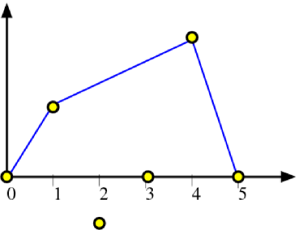
Fig. 1: Newton’s polygon for the polynomial $a(x)=x^{5}+10^{6}x^{4}+x^{3}+\frac{1}{100}x^{2}+10^{3}x+1$.

The effectiveness of this technique is explained in [3] where the following result is shown.

Theorem 2.

Under the assumptions of Theorem 1, it holds $p\leq q$,

$$\{h_{0},h_{1},\ldots,h_{p}\}\subset\{k_{0},k_{1},\ldots,k_{q}\}.$$

Moreover, $\{r_{1},\ldots,r_{q}\}\cap]s_{h_{j}},t_{h_{j}}[=\emptyset$ for $j=1,\ldots,p$.

Therefore, the approximations chosen in the previously described way lie in the union of the closed annuli $\mathcal{A}(t_{h_{i-1}},s_{h_{i}})$, $i=1,\ldots,p$ which, according to the Pellet theorem contain all the roots of all the polynomials having coefficients with the same moduli of the coefficients of $a(x)$. Moreover, the number of initial approximations chosen this way in each annulus coincides with the number of roots that the polynomial has in the same annulus. The advantage of this approach is that the computation of the Newton polygon and of the radii $r_{i}$ is almost inexpensive since it requires $O(n)$ operations, while computing the roots $s_{h_{i}}$ and $t_{h_{i}}$ is costly since it requires the solution of several polynomial equations. Recently, A. Melman [16] has proposed a cheap algorithm for approximating $s_{\kappa}$ and $t_{\kappa}$.

In [3] it is observed that any vertex $(k_{i},\log|a_{k_{i}}|)$ of the Newton polygon satisfies the following property

$$\begin{array}[]{l}u_{k_{i}}\leq v_{k_{i}},\quad v_{k_{i}}=u_{k_{i+1}}=r_{i+1},\quad i=0,\ldots,q-1,\\ u_{k_{i}}:=\max_{j<k_{i}}|a_{j}/a_{k_{i}}|^{1/(k_{i}-j)},\quad v_{k_{i}}:=\min_{j>k_{i}}|a_{j}/a_{k_{i}}|^{1/(k_{i}-j)}.\end{array}$$ (4)

In certain cases, the radii $r_{i}$ given by the Newton polygon provide approximations to the moduli of the roots which are better than the ones given by the Pellet theorem. The closeness of the radii $r_{i}$ to the moduli of the roots of $a(x)$, holds in particular when the radii differ relatively much from each other, or, equivalently, when the vertices of the Newton polygon are sufficiently sharp.

This has been recently proved by S. Gaubert and M. Sharify [8, 22]. In fact, using the theory of tropical polynomials, it turns out that the values $r_{i}$, for $i=1,\ldots,q$ coincide with the so called tropical roots of $a(x)$, and that the values $m_{i}=k_{i}-k_{i-1}$ are the multiplicities of the tropical roots $r_{i}$, for $i=1,\ldots,q$. This fact is used in [8, 22] to prove the following interesting result.

Theorem 3.

If $r_{i-1}/r_{i},r_{i}/r_{i+1}<1/9$, for $i=1,\ldots,p$, then any polynomial $b(x)$ having coefficients with the same modulus of the corresponding coefficients of $a(x)$ has $k_{i}-k_{i-1}$ roots in the annulus $\mathcal{A}(r_{i}/3,3r_{i})$.

That is, if three consecutive radii $r_{i-1},r_{i}$ and $r_{i+1}$ are sufficiently relatively far from each other, then the roots of any polynomial having coefficients with the same modulus of the corresponding coefficients of $a(x)$ are relatively close to the circle of center $0$ and radius $r_{i}$. This explains the good performances of the software MPSolve where only the sufficiently sharp vertices of the Newton polygon are considered for placing initial approximation to the roots.

An attempt to extend the Newton polygon technique to matrix polynomials is performed in [9] by relying on tropical algebra. The idea consists in associating with a matrix polynomial $A(x)=\sum_{i=0}^{n}A_{i}x^{i}$ the Newton polygon constructed from the scalar polynomial $w(x)=\sum_{i=0}^{n}\|A_{i}\|x^{i}$. An application of the results of [9] yields a scaling technique wich is shown to improve the backward stability of computing the eigenvalues of $A(x)$, particularly in situations where the data have various orders of magnitude. The same idea of relying on the Newton polygon constructed from $w(x)$ is used in [5] in the context of solving the polynomial eigenvalue problem with a root-finding approach.

Moreover, it is proved in [9] for the quadratic matrix polynomial and in [22, Chapter 4] for the general case, that under assumptions involving condition numbers, there is one group of “large” eigenvalues, which have a maximal order of magnitude, given by the largest tropical root. A similar result holds for a group of small eigenvalues. Recently it has been proved in [2] that the sequence of absolute values of the eigenvalues of $A(x)$ is majorized by a sequence of these tropical roots, $r_{i}$s. This extends to the case of matrix polynomials some bounds obtained by Hadamard [12], Ostrowski and Pólya [19, 20] for the roots of scalar polynomials. An attempt to extend Pellet’s theorem to matrix polynomial by relying on the Gerschgorin disks has been performed by A. Melman [17].

1.2 New results

In this paper we provide extension to matrix polynomials of Theorems 1, 2, 3 and arrive at an effective tool for selecting initial approximations to the eigenvalues of a matrix polynomial. This tool, coupled with the Ehrlich-Aberth iteration, provides a robust solver for the polynomial eigenvalue problem. A preliminary description of an implementation of this solver is given in [5].

The Pellet theorem is extended by considering the equations

$$x^{\kappa}=\sum_{i=0,\,i\neq\kappa}^{n}\|A_{\kappa}^{-1}A_{i}\|x^{i},$$

valid for all the $\kappa$ such that $\det A_{\kappa}\neq 0$, which have either 2 or no positive solutions for $\kappa=1,\ldots,n-1$ and the same equations for $\kappa=0$ and $\kappa=n$ which have one positive solution if $\det A_{0}\neq 0$ or $\det A_{n}\neq 0$, respectively.

The Newton polygon technique is extended by considering separately either the set of polynomials $\sum_{i=0}^{n}\|A_{\kappa}^{-1}A_{i}\|x^{i}$ for $\kappa$ such that $\det A_{\kappa}\neq 0$, or the single polynomial $\sum_{i=0}^{n}\|A_{i}\|x^{i}$. The latter case is subjected to the condition that $A_{i}$, $i=0,\ldots,n$ are well conditioned matrices.

Theorem 3 is extended to matrix polynomials such that $A_{i}=Q_{i}$, $Q_{i}Q_{i}^{*}=\sigma_{i}I$ for $i=0,\ldots,n$ where the constants 3 and 9 are replaced by slightly different values. For general polynomials, computational evidence shows that the bounds deteriorates when the condition number of coefficients increases.

The paper is organized as follows. In Section 2 we report the extensions of Theorems 1, 2, 3. Section 3 contains the proofs of these extension. Finally, Section 4 describes the results of the numerical experiments that confirm the effectiveness of our extensions.

2 The main extensions

Throughout the paper $A^{*}$ denotes the conjugate transpose of the matrix $A$, $\rho(A)$ is the spectral radius and $\|A\|=\rho(A^{*}A)^{1/2}$ is the 2-norm. We denote by ${\bf i}$ the imaginary unit such that ${\bf i}^{2}=-1$.

Define the class $\mathcal{P}_{m,n}$ of all the $m\times m$ matrix polynomials $A(x)=\sum_{i=0}^{n}A_{i}x^{i}$ with $A_{i}\in\mathbb{C}^{m\times m}$, satisfying the following properties:

• $A(x)$ is regular and has degree $n$, that is, $a(x)=\det A(x)$ is not identically zero and $A_{n}\neq 0$;

• $A_{0}\neq 0$.

The latter condition is no loss of generality. In fact, in this case we may just consider the polynomial $A(x)/x^{\kappa}$, where $\kappa$ is the smallest integer such that $A_{\kappa}\neq 0$.

Define also the class $\mathcal{Q}_{m,n}\subset\mathcal{P}_{m,n}$ such that

$$\mathcal{Q}_{m,n}=\{\sum_{i=0}^{n}A_{i}x^{i},\quad A_{i}=\sigma_{i}Q_{i},~{}~{}Q_{i}^{*}Q_{i}=I,~{}~{}\sigma_{i}\geq 0\}.$$ (5)

The class $\mathcal{Q}_{m,n}$ is given by all the matrix polynomials whose nonzero coefficients have unit spectral condition number. The expression $\sigma Q$ provides a first step in extending the complex number $\rho e^{{\bf i}\theta}$ to a matrix, where $\sigma$ plays the role of $\rho$ and $Q$ of $e^{{\bf i}\theta}$.

The following result provides a first extension of the Pellet theorem.

Theorem 4.

Let $A(x)\in\mathcal{P}_{m,n}$.

1. If $0<\kappa<n$ is such that $\det A_{\kappa}\neq 0$ then the equation

   $$x^{\kappa}=\sum_{i=0,\,i\neq\kappa}\|A_{\kappa}^{-1}A_{i}\|x^{i}$$ (6)

   has either no real positive solution or two real positive solutions $s_{\kappa}\leq t_{\kappa}$.

2. In the latter case, the polynomial $a(x)=\det A(x)$ has no roots in the inner part of the annulus $\mathcal{A}(s_{\kappa},t_{\kappa})$, while it has $m\kappa$ roots of modulus less than or equal to $s_{\kappa}$.

3. If $\kappa=0$ and $\det A_{0}\neq 0$ then (6) has only one real positive root $t_{0}$, moreover, the polynomial $a(x)$ has no root of modulus less than $t_{0}$.

4. If $\kappa=n$ and $\det A_{n}\neq 0$, then (6) has only one real positive solution $s_{n}$ and the polynomial $a(x)$ has no roots of modulus greater than $s_{n}$.

A consequence of the above result is given by the following corollary which provides a further extension of Theorem 1.

Corollary 5.

Let $h_{0}<h_{1}<...<h_{p}$ be the values of $\kappa$ such that $\det A_{\kappa}\neq 0$ and there exist positive real solution(s) of (6). Then

1. $t_{h_{i-1}}\leq s_{h_{i}}$, $i=1,\ldots,p$;

2. there are $m(h_{i}-h_{i-1})$ roots of $a(x)$ in the annulus $\mathcal{A}(t_{h_{i-1}},s_{h_{i}})$;

3. there are no roots of the polynomial $a(x)$ in the inner part of the annulus $\mathcal{A}(s_{h_{i}},t_{h_{i}})$, where $i=0,1,\ldots,p$ and we assume that $s_{h_{0}}=s_{0}:=0,t_{h_{p}}=t_{n}:=\infty$.

Observe that in the case where $m=1$, i.e., the matrix polynomial is a scalar polynomial, Corollary 5 coincides with Theorem 1. Moreover, the bounds to the moduli of the eigenvalues of $A(x)$ given in the above results are strict since there exist matrix polynomials, say, polynomials with coefficients $A_{i}=\sigma_{i}I$, which attain these bounds.

Theorem 4 improves [13, Lemma 3.1] where the upper and lower bounds to the moduli of the eigenvalues of a matrix polynomial are given by the positive solutions of the polynomial equations

$$\begin{split}x^{n}&=\sum_{i=0}^{n-1}\|A_{i}\|\|A_{n}^{-1}\|x^{i};\\ 1&=\sum_{i=1}^{n}\|A_{i}\|\|A_{0}^{-1}\|x^{i}.\end{split}$$

The improvement comes from the simple observation that $\|AB\|\leq\|A\|\|B\|$ for any pair of square matrices $A,B$.

If $\det A_{0}=0$, clearly the lower bound $t_{0}$ on the modulus of the roots of $a(x)$ stated in part 3 of Theorem 4 is missing. In fact, there is at least one eigenvalue of $A(x)$ equal to zero. Similarly, if $\det A_{n}=0$ there is no upper bound $s_{n}$ to the modulus of the roots of $a(x)$ stated in part 4 of Theorem 4. In fact, in this case there exist infinite eigenvalues.

Notice that in Corollary 5 the value $h_{0}=0$ exists if $\det A_{0}\neq 0$, and the value $h_{p}=n$ exists if $\det A_{n}\neq 0$. However, if the remaining coefficients $A_{\kappa}$, for $\kappa=1,\ldots,n-1$, even though non-singular, are very ill-conditioned, then it may happen that the set $\{h_{1},\ldots,h_{p-1}\}$ is empty so that Corollary 5 does not provide much information.

If $A(x)\in\mathcal{Q}_{m,n}$, then the following extension of Theorem 1 holds.

Theorem 6.

Let $A(x)\in\mathcal{Q}_{m,n}$ so that $A_{i}=\sigma_{i}Q_{i}$ and $Q_{i}^{*}Q_{i}=I$. Let $s_{h_{i}},t_{h_{i}}$, $i=1,\ldots,p$ be the quantities given by Theorem 1 applied to $w(x)=\sum_{i=0}^{n}\sigma_{i}x^{i}$. Then any matrix polynomial $B(x)=\sum_{i=0}^{n}\sigma_{i}S_{i}x^{i}\in\mathcal{Q}_{m,n}$ for $S_{i}^{*}S_{i}=I$, has

1. $m(h_{i}-h_{i-1})$ eigenvalues in the annulus $\mathcal{A}(t_{h_{i-1}},s_{h_{i}})$;

2. no eigenvalues with modulus in the inner part of the annulus $\mathcal{A}(s_{h_{i}},t_{h_{i}})$.

2.1 The Newton polygon technique

The results given in the previous subsection provide a useful tool for selecting initial approximations to the eigenvalues of $A(x)$ to be refined by a polynomial root-finder based on simultaneous iterations. However, we may avoid to compute roots of polynomials and rely on the Newton polygon construction.

In this section we provide some new results by using the Newton polygon technique. We start by stating the following theorem.

Theorem 7.

Let $A(x)\in\mathcal{P}_{m,n}$. If $\kappa$ is such that (6) has two real positive solutions $s_{\kappa}\leq t_{\kappa}$, then $u_{\kappa}\leq s_{\kappa}\leq t_{\kappa}\leq v_{\kappa}$ where

$$\begin{array}[]{l}u_{\kappa}:=\max_{i<\kappa}||A_{\kappa}^{-1}A_{i}||^{1/(\kappa-i)},\\[4.30554pt] v_{\kappa}:=\min_{i>\kappa}||A_{\kappa}^{-1}A_{i}||^{1/(\kappa-i)}\end{array}$$

If $\det A_{0}\neq 0$ then for $\kappa=0$ (6) has a solution $t_{0}$ and

$$t_{0}\leq v_{0}:=\min_{i>0}||A_{0}^{-1}A_{i}||^{-1/i}$$

If $\det A_{n}\neq 0$ then for $\kappa=n$ (6) has a solution $s_{n}$ and

$$s_{n}\geq u_{n}:=\max_{i<n}||A_{n}^{-1}A_{i}||^{1/(n-i)}$$

Observe that for scalar polynomials the values $u_{k_{i}}$ and $v_{k_{i}}$ are such that $v_{k_{i}}=u_{k_{i+1}}=r_{i}$, where $r_{i}$ are defined in (3) and $k_{i}$ are the abscissas of the vertices of the Newton polygon.

The following result extends Theorem 2 to matrix polynomials.

Theorem 8.

Given $A(x)\in\mathcal{P}_{m,n}$, let $\mathcal{S}=\{k_{i}:\quad i=0,...,q\}$ be such that $u_{\kappa}<v_{\kappa}$ if and only if $\kappa\in\mathcal{S}$, where $u_{\kappa}$ and $v_{\kappa}$ are defined in Theorem 7. Then,

1. $p\leq q$ and $\{h_{0},...,h_{p}\}\subseteq\{k_{0},...,k_{q}\}$;

2. $\left(\{u_{1},...,u_{q}\}\cup\{v_{1},\ldots,v_{q}\}\right)\cap[s_{k_{i}},t_{k_{i}}]=\emptyset$;

3. $v_{k_{i}}\leq u_{k_{i+1}}$, $i=0,\ldots,q-1$;

4. if $A(x)\in\mathcal{Q}_{m,n}$, then $v_{k_{i}}=u_{k_{i+1}}$ and $v_{k_{i}}$ coincide with the vertices of the Newton polygon of the polynomial $w(x)=\sum_{i=0}^{n}\|A_{i}\|x^{i}=\sum_{i=0}^{n}\sigma x^{i}$.

Therefore, the strategy of choosing $m(k_{i}-k_{i-1})$ approximations placed along the circle of center 0 and radius either $r_{i}=v_{k_{i}}$ or $r_{i}=u_{k_{i+1}}$ is effective. In fact, these approximations lie in the union of the closed annuli $\mathcal{A}_{i}$ of radii $t_{h_{i-1}}$ and $s_{h_{i}}$, $i=1,\ldots,p$, in the complex plane which, according to the extension of the Pellet theorem, contain all the eigenvalues of $A(x)$. The computation of the radii $r_{i}$ is cheap since it is reduced to compute the values $k_{i}$, $i=0,\ldots,q$ defined in Theorem 8 by evaluating the quantities $u_{k_{i}}$ and $v_{k_{i}}$ defined in Theorem 7. In the case of polynomials in $\mathcal{Q}_{m,n}$ this computation is even cheaper since it is reduced to computing the Newton polygon of the polynomial $w(x)$.

Observe that for general matrix polynomials, $u_{k_{i+1}}$ does not generally coincide with $v_{k_{i}}$ nor with the values obtained by computing the Newton polygon of $w(x)$. However, in the practice of the computations, when the matrix coefficients corresponding to the vertices are well conditioned, there is not much difference between the values obtained in these different ways.

The effectiveness of this strategy of selecting starting approximations is strengthened by the following result which generalizes Theorem 3.

Theorem 9.

Let $A(x)=\sum_{i=0}^{n}\sigma_{i}Q_{i}x^{i}\in\mathcal{Q}_{m,n}$ be a matrix polynomial of degree $n$ and let $r_{1},\dots,r_{q}$ denote the radii of the Newton polygon associated with the polynomial $w(x)=\sum_{i=0}^{n}\sigma_{i}x^{i}$. Also, let $k_{0},\dots,k_{q}$ be the abscissas of the vertices of the Newton polygon and set $m_{i}=k_{i}-k_{i-1}$. There exist constants $f,g$ such that $12.11<f<12.12$, $4.371<g<4.372$ and

1. for $1<i<q$, if $r_{i-1}/r_{i},\,r_{i}/r_{i+1}<1/f$, then $A(x)$ has exactly $mm_{i}$ eigenvalues in the annulus $\mathcal{A}(r_{i}/g,r_{i}g)$;

2. for $i=1$, if $r_{i}/r_{i+1}<1/f$ then, $A(x)$ has exactly $mm_{i}$ eigenvalues in the annulus $\mathcal{A}(r_{i}/g^{\prime},r_{i}g)$, where $g^{\prime}=2+\sqrt{2}$;

3. for $i=q$, if $r_{i-1}/r_{i}<1/f$ then, $A(x)$ has exactly $mm_{i}$ eigenvalues in the annulus $\mathcal{A}(r_{i}/g,r_{i}g^{\prime})$.

Observe that in the scalar case the values of the constants $f$ and $g$ are given by $f=9$ and $g=3$ which are slightly better.

3 The proofs

The key tool on which the proofs of our results rely is the generalization of Rouché theorem to the case of matrix polynomials provided in [10], see also [23]. In this statement and throughout, we use the notation $H\succ 0$ if the Hermitian matrix $H$ is positive definite.

Theorem 10.

Let $P(x)$ and $Q(x)$ be square matrix polynomials, and $\Gamma$ be a simple closed Jordan curve. If $P(x)^{*}P(x)-Q(x)^{*}Q(x)\succ 0$ for all $x\in\Gamma$, then the polynomials $p(x):=\det(P(x))$ and $f(x):=\det(P(x)+Q(x))$ have the same number of roots in the open set bounded by $\Gamma$.

We provide the proofs of the results listed in Section 2. Assume that $\det A_{\kappa}\neq 0$ and consider the matrix polynomial $\widehat{A}(x)=\sum_{i=0}^{n}A_{\kappa}^{-1}A_{i}x^{i}$ which has the same eigenvalues as $A(x)$. We start simply by applying Theorem 10 to the matrix polynomials $P(x)=x^{\kappa}I$ and $Q(x)=\widehat{A}(x)-P(x)$ where $\Gamma$ is the circle of center $0$ and radius $r$.

The condition $P(x)^{*}P(x)-Q(x)^{*}Q(x)\succ 0$ turns into $|x|^{2\kappa}I-Q(x)^{*}Q(x)\succ 0$. Moreover, since

$$\begin{split}\rho(Q(x)^{*}Q(x))=&\|Q(x)^{*}Q(x)\|\leq\|Q(x)^{*}\|\cdot\|Q(x)\|=\|Q(x)\|^{2}\\ \leq&(\sum_{i=0,\,i\neq\kappa}^{n}\|A_{\kappa}^{-1}A_{i}\|\cdot|x|^{i})^{2},\end{split}$$

we deduce that the condition $P(x)^{*}P(x)-Q(x)^{*}Q(x)\succ 0$ is implied by

$$|x|^{\kappa}>\sum_{i=0,\,i\neq\kappa}^{n}\|A_{\kappa}^{-1}A_{i}\|\cdot|x|^{i}.$$ (7)

Thus, we may conclude with the following

Lemma 11.

If (7) is satisfied for $|x|=r$, then $A(x)$ has $m\kappa$ eigenvalues in the disk of center 0 and radius $r$.

Proof.

If (7) is satisfied for $|x|=r$, then $P(x)P^{*}(x)\succ Q(x)Q^{*}(x)$ for $P(x)=x^{\kappa}I$, $Q(x)=\widehat{A}(x)-P(x)$ and $|x|=r$. Therefore, by Theorem 10, the matrix polynomial $P(x)+Q(x)=\widehat{A}(x)$ has as many eigenvalues of modulus less than $r$ as the matrix polynomial $P(x)=x^{\kappa}I$, that is $m\kappa$. ∎

We recall this known result which in [3] is proved by induction on $\kappa$.

Lemma 12.

Let $w(x)=\sum_{i=0}^{n}w_{i}x^{i}$, $w_{0},w_{n}>0$, $w_{i}\geq 0$. The equation $w_{\kappa}x^{\kappa}=\sum_{i=0,\,i\neq\kappa}^{n}w_{i}x^{i}$ has only one real positive solution if $\kappa\in\{0,n\}$, and either 2 or no real positive solutions if $0<\kappa<n$.

Applying Lemma 12 to the equation $x^{\kappa}=\sum_{i=0,\,i\neq\kappa}^{n}\|A_{\kappa}^{-1}A_{i}\|\cdot x^{i}$, in view of Lemma 11 one obtains Theorem 4.

Now, consider the set of indices $\mathcal{H}=\{h_{0}<h_{1}<\ldots<h_{p}\}$ such that $\det A_{\kappa}\neq 0$ and the equation

$$x^{\kappa}=\sum_{i=0,\,i\neq\kappa}^{n}\|A_{\kappa}^{-1}A_{i}\|\cdot x^{i}.$$

has real positive solutions for $\kappa\in\mathcal{H}$. Denote $s_{h_{i}}\leq t_{h_{i}}$, $i=0,\ldots,p$ these solutions, where we have set $s_{h_{0}}=0$ and $t_{h_{p}}=\infty$. Observe that if $\det A_{0}\neq 0$ then $h_{0}=0$ and if $\det A_{n}\neq 0$ then $h_{p}=n$.

By applying Theorem 4 one deduces that the closed disk of center 0 and radius $s_{h_{i}}$ contains exactly $mh_{i}$ eigenvalues of $A(x)$ for $i=1,\ldots,p$, while there are none in the inner part of the annulus $\mathcal{A}(s_{h_{i}},t_{h_{i}})$. This implies that $s_{h_{i+1}}\geq t_{h_{i}}$, that is, part 1 of Corollary 5, and that there are $m(h_{i}-h_{i-1})$ eigenvalues in the annulus $\mathcal{A}(t_{h_{i-1}},s_{h_{i}})$, i.e., part 2 of Corollary 5. Part 3 follows from a direct application of Theorem 4 so that the proof of Corollary 5 is complete.

In the case where the matrix polynomial $A(x)$ belongs to $\mathcal{Q}_{m,n}$, we find that $A_{\kappa}^{-1}A_{i}=(\sigma_{i}/\sigma_{\kappa})I$ so that condition (7) turns into

$$|x|^{\kappa}>\sum_{i=0,\,i\neq\kappa}^{n}\left|\frac{\sigma_{i}}{\sigma_{\kappa}}\right|\cdot|x|^{i}.$$

This way, the proof of Theorem 6 follows from Theorem 4.

3.1 Proofs related to the Newton polygon

Assume that $0<\kappa<n$ and that equation (6) has real positive solutions $s_{\kappa}\leq t_{\kappa}$. Then, for any $x\in\{s_{\kappa},t_{\kappa}\}$ one has

$$x^{\kappa}=\sum_{i=0,\,i\neq\kappa}^{n}\|A_{\kappa}^{-1}A_{i}\|x^{i}\geq\|A_{\kappa}^{-1}A_{j}\|x^{j}$$

for any $j\neq\kappa$. This implies that $x\geq\max_{j<\kappa}\|A_{\kappa}^{-1}A_{j}\|^{1/(\kappa-j)}=u_{\kappa}$ and $x\leq\min_{j>\kappa}\|A_{\kappa}^{-1}A_{j}\|^{1/(\kappa-j)}=v_{\kappa}$. This proves the first part of Theorem 7. The cases $\kappa=0$ and $\kappa=n$ are treated similarly.

Now consider Theorem 8. Parts 1 and 2 follow from Theorem 7. Concerning the inequality $v_{k_{i}}\leq u_{k_{i+1}}$, we rely on the property $\|H\|\geq 1/\|H^{-1}\|$ valid for any non-singular matrix $H$. In fact, for the sake of simplicity, denote $k:=k_{i}$ and $h:=k_{i+1}$ so that $k<h$. Then

$$\begin{split}u_{h}=&\max_{j<h}\|A_{h}^{-1}A_{j}\|^{1/(h-j)}\geq\|A_{h}^{-1}A_{k}\|^{1/(h-k)}\geq\|(A_{h}^{-1}A_{k})^{-1}\|^{-1/(h-k)}\\ &\geq\min_{j>k}\|(A_{j}^{-1}A_{k})^{-1}\|^{-1/(j-k)}=\min_{j>k}\|A_{k}^{-1}A_{j}\|^{1/(k-j)}=v_{k}.\end{split}$$

Concerning part 4, if $A(x)\in\mathcal{Q}_{m,n}$, then in view of Theorem 6, the values of $k_{i}$ are the abscissas of the vertices of the Newton polygon for the polynomial $w(x)=\sum_{i=0}^{n}\sigma_{i}x^{i}$, therefore $v_{k_{i}}=u_{k_{i+1}}$, and the proof of Theorem 8 is complete.

3.2 Proof of Theorem 9

Let $A(x)=\sum_{i=0}^{n}\sigma_{i}Q_{i}\in\mathcal{Q}_{m,n}$ and $w(x)=\sum_{i=0}^{n}\sigma_{i}x^{i}$. Consider the Newton polygon corresponding to $w(x)$ where $k_{i-1},k_{i}$ are the abscissas of two consecutive vertices corresponding to the $i$th edge. Also, let $r_{1},\dots,r_{q}$, denote the radii corresponding to different edges of the Newton polygon so that $r_{1}<r_{2}<\dots<r_{q}$. Along the proof we refer to the radii as the tropical roots. Also, for the sake of notational simplicity we set $k:=k_{i-1}$ and $h:=k_{i}$.

Let $r_{i}$ be the tropical root corresponding to the $i$th edge of the Newton polygon and consider the substitution $y=r_{i}x$. We define the matrix polynomial $\tilde{A}(y)=\sum_{j=0}^{n}\tilde{A_{j}}y^{j}$ as follows:

$$\tilde{A}(y)=(\sigma_{k}r_{i}^{k})^{-1}(\sum_{j=0}^{n}A_{j}(r_{i}y)^{j})\enspace.$$ (8)

Notice that $\lambda$ is an eigenvalue of $\tilde{A}(y)$ if and only if $r_{i}\lambda$ is an eigenvalue of $A(x)$. The scaled matrix polynomial $\tilde{A}(y)$ has the following property.

Lemma 13 (Corollary of [22, Lemma 3.3.2]).

Let $\tilde{A}(y)$ be the matrix polynomial defined in (8) and let $\tilde{\sigma_{j}}:=\|\tilde{A_{j}}\|$ for $j=0,\dots,n$. Also let $\epsilon:=r_{i-1}/r_{i}$, $\delta:=r_{i}/r_{i+1}$, be the parameters measuring the separation between $r_{i}$ and the previous and the next tropical roots, $r_{i-1}$ and $r_{i+1}$, respectively. We have:

$$\tilde{\sigma_{j}}\leq\begin{cases}\epsilon^{k-j}&\mathrm{if}\quad j<k,\\ 1&\mathrm{if}\quad k\leq j\leq h,\\ \delta^{j-h}&\mathrm{if}\quad j>h.\end{cases}$$

Proof.

We only prove the first inequality since the other ones can be established by using a similar argument. Note that $\tilde{\sigma_{j}}=(\sigma_{k}r_{i}^{k})^{-1}\sigma_{j}r_{i}^{j}$. Due to [22, Lemma 3.3.2], $\sigma_{j}\leq\sigma_{k}r_{i-1}^{k-j}$ for all $0\leq j<k$. Thus,

$$\tilde{\sigma_{j}}\leq(\sigma_{k}r_{i}^{k})^{-1}\sigma_{k}r_{i-1}^{k-j}r_{i}^{j}=(\frac{r_{i-1}}{r_{i}})^{k-j}=\epsilon^{k-j}.$$

∎

Now consider the decomposition of $\tilde{A}(y)$ as the sum of two matrix polynomials:

$$P(y)=\sum_{j=k}^{h}\tilde{A}_{j}y^{j},\qquad Q(y)=\sum_{j=0}^{k-1}\tilde{A}_{j}y^{j}+\sum_{j=h+1}^{n}\tilde{A}_{j}y^{j}\enspace.$$

Remark 14.

Notice that, although for the sake of notational simplicity we do not explicitly express this dependence, the definitions of $\tilde{A}(y)$, $P(y)$ and $Q(y)$ depend on which edge of the Newton polygon we are considering.

The following lemma provides the upper and lower bounds to the moduli of the eigenvalues of $P(y)$.

Lemma 15 (Corollary of [13, Lemma 4.1]).

All the nonzero eigenvalues of $P(y)$ lie in the annulus $\mathcal{A}(1/2,2)$.

Proof.

Consider the polynomial $y^{-k}P(y)$. Due to [13, Lemma 4.1] we have:

$$(1+\|\tilde{A}_{k}^{-1}\|)^{-1}\min_{k\leq j\leq h}\|\tilde{A}_{j}\|^{-1/j}\leq|\lambda|\leq(1+\|\tilde{A}_{h}^{-1}\|)\max_{k\leq j\leq h}\|\tilde{A}_{j}\|^{1/(h-k-j)}$$

where $\lambda$ is any eigenvalue of $y^{-k}P(y)$. The result is established by applying Lemma 13 to the above inequalities. ∎

The idea of the proof is to look for the conditions on $\epsilon=r_{i-1}/r_{i}$ and $\delta=r_{i}/r_{i+1}$ such that $P(y)^{*}P(y)-Q(y)^{*}Q(y)\succ 0$ holds on the boundaries of two disks of center zero and radius $r_{1}<1/2$ and $r_{2}>2$. Then, by the generalized Rouché theorem (Theorem 10), $P(y)$ and $\tilde{A}(y)$ will have the same number of eigenvalues inside these disks. Using Lemma 15, this implies that $\tilde{A}(y)$ has $m(h-k)$ eigenvalues which lie in the annulus $\mathcal{A}(r_{1},r_{2})$; therefore, $A(x)$ has $m(h-k)$ eigenvalues which lie in the annulus $\mathcal{A}(r_{i}r_{1},r_{i}r_{2})$. This argument is akin to the one which is used in [22, Chapter 3] to prove Theorem 3, valid for scalar polynomials. The proof relies on the following lemmas.

Lemma 16.

Let $r:=|y|$ and $\ell:=h-k$. Also, define the diagonal matrices $D_{i}=d_{i}I_{m}$, $i=1,\dots,3$, and the Hermitian matrices $H_{i}$, $i=1\dots 4$, as follows:

$$D_{1}(y) := (\sum_{j=k}^{h}\|\tilde{A}_{j}\|^{2}|y|^{2j})I_{m}\enspace,\quad D_{2}(y):=(\sum_{j=0}^{k-1}\|\tilde{A}_{j}\|^{2}|y|^{2j})I_{m}\enspace,$$

$$D_{3}(y) := (\sum_{j=h+1}^{n}\|\tilde{A}_{j}\|^{2}|y|^{2j})I_{m}\enspace;$$

$$H_{1}(y) := \sum_{k\leq j_{1}<j_{2}\leq h}\tilde{A}_{j_{1}}^{*}\tilde{A}_{j_{2}}(y^{*})^{j_{1}}y^{j_{2}}+\left(\sum_{k\leq j_{1}<j_{2}\leq h}\tilde{A}_{j_{1}}^{*}\tilde{A}_{j_{2}}(y^{*})^{j_{1}}y^{j_{2}}\right)^{*},$$

$$H_{2}(y) := \sum_{0\leq j_{1}<j_{2}\leq k-1}\tilde{A}_{j_{1}}^{*}\tilde{A}_{j_{2}}(y^{*})^{j_{1}}y^{j_{2}}+\left(\sum_{0\leq j_{1}<j_{2}\leq k-1}\tilde{A}_{j_{1}}^{*}\tilde{A}_{j_{2}}(y^{*})^{j_{1}}y^{j_{2}}\right)^{*},$$

$$H_{3}(y) := \sum_{h+1\leq j_{1}<j_{2}\leq n}\tilde{A}_{j_{1}}^{*}\tilde{A}_{j_{2}}(y^{*})^{j_{1}}y^{j_{2}}+\left(\sum_{h+1\leq j_{1}<j_{2}\leq n}\tilde{A}_{j_{1}}^{*}\tilde{A}_{j_{2}}(y^{*})^{j_{1}}y^{j_{2}}\right)^{*},$$

$$H_{4}(y) := \sum_{j_{1}=0}^{k-1}\sum_{j_{2}=h+1}^{n}\tilde{A}_{j_{1}}^{*}\tilde{A}_{j_{2}}(y^{*})^{j_{1}}y^{j_{2}}+\left(\sum_{j_{1}=0}^{k-1}\sum_{j_{2}=h+1}^{n}\tilde{A}_{j_{1}}^{*}\tilde{A}_{j_{2}}(y^{*})^{j_{1}}y^{j_{2}}\right)^{*}.$$

Then we have:

1. $[P(y)]^{*}P(y)-[Q(y)]^{*}Q(y)=D_{1}(y)+H_{1}(y)-D_{2}(y)-D_{3}(y)-H_{2}(y)-H_{3}(y)-H_{4}(y)$;

2. if $r>1$, $d_{1}\geq r^{2h}\frac{r^{2}-2+r^{-2\ell}}{r^{2}-1}$;

3. if $r<1$, $d_{1}\geq r^{2k}\frac{1-2r^{2}+r^{2\ell+2}}{1-r^{2}}$;

4. $\|H_{1}\|\leq 2r^{k+1}\frac{r^{2h-k+1}-r^{h+1}-r^{h}+r^{k}}{(r^{2}-1)(r-1)}$;

5. $d_{2}+d_{3}+\sum_{i=2}^{4}\|H_{i}\|\leq\left(\epsilon\frac{\epsilon^{k}-r^{k}}{\epsilon-r}+\delta r^{h+1}\frac{1-(r\delta)^{n-h}}{1-r\delta}\right)^{2}$.

Proof.

The first equation is easily verified by direct computation.

The proofs of inequalities 2. and 3. have been presented in [22, Lemma 3.3.5].

1. Note that

   $$\|H_{1}\|\leq 2\sum_{k\leq j_{1}<j_{2}\leq h}\|\tilde{A}_{j_{1}}\|\|\tilde{A}_{j_{2}}\|r^{j_{1}+j_{2}} \leq 2\sum_{k\leq j_{1}<j_{2}\leq h}r^{j_{1}+j_{2}}\quad{\textit{ (using Lemma~{}\ref{lem3})}}$$

   $$= 2(1-r)^{-1}\sum_{j_{1}=k}^{h-1}r^{2j_{1}+1}(1-r^{h-j_{1}})\enspace.$$

   Taking the sum over $j_{1}$ completes the proof.

2. It follows from Lemma 13 that

   $$d_{2}\leq\epsilon^{2k}\sum_{j=0}^{k-1}(r/\epsilon)^{2j},\quad d_{3}\leq\delta^{-2h}\sum_{j=h+1}^{n}(\delta r)^{2j},\quad\|H_{2}\|\leq 2\epsilon^{2k}\sum_{0\leq j_{1}<j_{2}\leq k-1}(r/\epsilon)^{j_{1}+j_{2}},$$

   $$\|H_{3}\|\leq 2\delta^{-2h}\sum_{h+1\leq j_{1}<j_{2}\leq n}(\delta r)^{j_{1}+j_{2}},\quad\|H_{4}\|\leq 2\epsilon^{k}\delta^{-h}\sum_{j_{1}=0}^{k-1}\sum_{j_{2}=h+1}^{n}(r/\epsilon)^{j_{1}}(r\delta)^{j_{2}}.$$

   Then we have

   $$d_{2}+d_{3}+\sum_{i=2}^{4}\|H_{i}\|\leq\big{(}\epsilon^{k}\sum_{j=0}^{k-1}(r/\epsilon)^{j}+\delta^{-h}\sum_{j=h+1}^{n}(\delta r)^{j}\big{)}^{2}\enspace.$$

   The proof is achieved by computing the right hand side of the above inequality.

∎

Lemma 17.

For any edge $i=1,\dots,q-1$ of the Newton polygon, if $\delta=r_{i}/r_{i+1}<1/f$, where $12.11<f<12.12$, then $\tilde{A}(y)$ and $P(y)$ have the same number of eigenvalues in the disk centered at zero and with radius $g$, where $4.371<g<4.372$. For the last edge of the Newton polygon where $i=q$, $\tilde{A}(y)$ and $P(y)$ have the same number of eigenvalues in the disk centered at zero with radius $g>2+\sqrt{2}$.

Proof.

Along the proof we assume that $r>1$. Using Lemma 16, a sufficient condition for $[P(y)]^{*}P(y)-[Q(y)]^{*}Q(y)\succ 0$ is that

$$d_{1}>d_{2}+d_{3}+\rho(-H_{1}+H_{2}+H_{3}+H_{4})\enspace.$$ (9)

Since $\rho(-H_{1}+H_{2}+H_{3}+H_{4})\leq\sum_{i=1}^{4}\|H_{i}\|$,  (9) is implied by

$$d_{1}-\|H_{1}\|>d_{2}+d_{3}+\sum_{i=2}^{4}\|H_{i}\|\enspace.$$ (10)

Observe that, by Lemma 16,

$$d_{1}-\|H_{1}\|\geq r^{2h}\big{(}\frac{r^{2}-4r+2}{(r-1)^{2}}+\frac{2r^{-\ell+1}-r^{-2\ell}}{(r-1)^{2}}\big{)}\enspace.$$

Thus, (10) is deduced from the following inequality:

$$\frac{r^{2}-4r+2}{(r-1)^{2}}+\frac{2r^{-\ell+1}-r^{-2\ell}}{(r-1)^{2}}>\left[\epsilon\ \frac{r^{-\ell}-\epsilon^{k}r^{-h}}{r-\epsilon}+\delta r\ \frac{1-(\delta r)^{n-h}}{1-\delta r}\right]^{2}.$$ (11)

Assume now that $\delta r<1$; since $\epsilon<1$ we get

$$\left[\epsilon\ \frac{r^{-\ell}-\epsilon^{-\ell}}{r-\epsilon}+\delta r\ \frac{1-(\delta r)^{n-h}}{1-\delta r}\right]^{2}\leq\left[\frac{r^{-\ell}}{r-1}+\frac{\delta r}{1-\delta r}\right]^{2}\quad\enspace.$$

Then (11) follows from

$$\frac{r^{2}-4r+2}{(r-1)^{2}}+\frac{2r^{-\ell+1}-r^{-2\ell}}{(r-1)^{2}}>\left[\frac{r^{-\ell}}{r-1}+\frac{\delta r}{1-\delta r}\right]^{2}\enspace,$$ (12)

which is equivalent to

$$\frac{r^{2}-4r+2}{(r-1)^{2}}+2r^{-2\ell}\frac{r^{\ell+1}-1+\delta r^{\ell+1}-2\delta r^{\ell+2}+\delta r}{(r-1)^{2}(1-\delta r)}>(\frac{\delta r}{1-\delta r})^{2}\enspace.$$ (13)

Now, assume that $\delta\leq\frac{1}{2r}$; since $\ell\geq 1$, we have

$$r^{\ell+1}-1+\delta r^{\ell+1}-2\delta r^{\ell+2}+\delta r\geq r^{\ell+1}-1-2\delta r^{\ell+2}+2\delta r=(r^{\ell+1}-1)(1-2\delta r)\geq 0\enspace.$$

Then (13) follows from the following inequality:

$$\frac{r^{2}-4r+2}{(r-1)^{2}}>\frac{\delta^{2}r^{2}}{(1-\delta r)^{2}}\enspace,$$ (14)

which can be written in the polynomial form

$$p(\delta):=a(r)\delta^{2}+b(r)\delta+c(r)>0,$$

where $a(r):=r^{2}(1-2r)$, $b(r):=-2rc(r)$, $c(r):=r^{2}-4r+2$. Note first that $r>1$ implies $a(r)<0$; let us consider the discriminant of $p(\delta)$, i.e. $\Delta(r):=[b(r)]^{2}-4a(r)c(r)=4r^{2}(r-1)^{2}c(r)$. We see that $\Delta(r)$ cannot be negative, otherwise $p(\delta)<0\ \forall r>1$. Thus, it must hold $c(r)>0$, which implies that $r>2+\sqrt{2}$.

We deduce that $p(\delta)>0$ for all the values of $\delta$ which satisfy

$$\delta<\delta_{+}(r):=\frac{-c(r)+(r-1)\sqrt{c(r)}}{r(2r-1)}\enspace.$$ (15)

The graph of $\delta_{+}(r)$ is demonstrated in Figure 2.

Fig. 2: The graph of $\delta_{+}(r)$ as a function of $r$.

The maximum value of $\delta_{+}(r)$ is $\delta_{\max}=\frac{7+3\sqrt{3}}{2}-\sqrt{18+\frac{21\sqrt{3}}{2}}\simeq 0.08255\simeq\frac{1}{12.1136}$ which is obtained at $r=r_{0}:=\frac{3+\sqrt{3}}{2}+\sqrt{2+\frac{7\sqrt{3}}{6}}\simeq 4.3712$. So for $\delta<\delta_{\max}$ inequality (14) holds, which implies that $[P(y)]^{*}P(y)-[Q(y)]^{*}Q(y)\succ 0$ on the boundary of a disk of radius $r_{0}\simeq 4.3712$. Then, by the Rouché theorem (Theorem 10), $P(y)$ and $\tilde{A}(y)=P(y)+Q(y)$ have the same number of zeros inside a disk of radius $r_{0}$. This completes the proof of the first part of the lemma.

Note now that for the last edge of the Newton polygon, since the terms $D_{3},H_{3},H_{4}$ are zero, inequality (12) becomes

$$\frac{r^{2}-4r+2}{(r-1)^{2}}+\frac{2r^{-\ell+1}-r^{-2\ell}}{(r-1)^{2}}>\left[\frac{r^{-\ell}}{r-1}\right]^{2}\enspace,$$

or equivalently, $r^{2}-4r+2+2r^{-\ell+1}-2r^{-2\ell}>0$ which holds for any $r>2+\sqrt{2}$. ∎

Lemma 18.

For any edge $i=2,\dots,q$ of the Newton polygon, if $\epsilon=r_{i-1}/r_{i}<1/f$, where $12.11<f<12.12$, then $\tilde{A}(y)$ and $P(y)$ have the same number of eigenvalues in the disk centered at zero and with radius $1/g$, where $4.371<g<4.372$. For the first edge of the Newton polygon where $i=1$, $\tilde{A}(y)$ and $P(y)$ have the same number of eigenvalues in the disk centered at zero, with radius $1/g$ where $g>2+\sqrt{2}$.

Proof.

Along the proof we assume that $r<1$. We follow a similar argument to the previous lemma: the formulae that we will obtain are akin to those that we had gotten for the case $r>1$. We will therefore give fewer details.

Starting from (10) we get:

$$\frac{2r^{2}-4r+1}{(1-r)^{2}}+\frac{2r^{l+1}-r^{2l+2}}{(1-r)^{2}}>\left[\epsilon\frac{1-(\epsilon r^{-1})^{k}}{r-\epsilon}+\delta r^{l+1}\ \frac{1-(\delta r)^{n-h}}{1-\delta r}\right]^{2},$$ (16)

which is analogous to (11). Assume that $\epsilon<r$; we have

$$\left[\epsilon\frac{1-(\epsilon r^{-1})^{k}}{r-\epsilon}+\delta r^{l+1}\ \frac{1-(\delta r)^{n-h}}{1-\delta r}\right]^{2}\leq\left[\frac{\epsilon}{r-\epsilon}+\frac{\delta r^{l+1}}{1-\delta r}\right]^{2}\leq\left[\frac{\epsilon}{r-\epsilon}+\frac{r^{l+1}}{1-r}\right]^{2}\enspace.$$

Thus,  (16) is deduced from the following inequality:

$$\frac{2r^{2}-4r+1}{(1-r)^{2}}+\frac{2r^{l+1}-r^{2l+2}}{(1-r)^{2}}>\left[\frac{\epsilon}{r-\epsilon}+\frac{r^{l+1}}{1-r}\right]^{2}\enspace,$$ (17)

which is equivalent to

$$\frac{2r^{2}-4r+1}{(1-r)^{2}}+2r^{l+1}\frac{r-r^{l+2}-2\epsilon+\epsilon r^{l+1}+\epsilon r}{(1-r)^{2}(r-\epsilon)}>\frac{\epsilon^{2}}{(r-\epsilon)^{2}}\enspace.$$ (18)

Now assume that $\epsilon<\frac{r}{2}$; we have

$$r-r^{l+2}-2\epsilon+\epsilon r^{l+1}+\epsilon r\geq r-r^{l+2}+2\epsilon r^{l+1}-2\epsilon=(1-r^{\ell+1})(r-2\epsilon)>0\enspace.$$

Thus,  (18) is deduced from

$$\frac{2r^{2}-4r+1}{(1-r)^{2}}>\frac{\epsilon^{2}}{(r-\epsilon)^{2}}\enspace.$$

Setting $\rho=r^{-1}$ we get inequality (14) and, following the arguments already used in the proof of Lemma 17, we find a maximal value equal to $\epsilon_{\max}=\frac{7+3\sqrt{3}}{2}-\sqrt{18+\frac{21\sqrt{3}}{2}}\simeq 0.08255\simeq\frac{1}{12.1136}$, which is obtained at $r=r_{0}^{-1}=\frac{3-\sqrt{3+2\sqrt{3}}}{2}\simeq 0.22877\simeq\frac{1}{4.3712}$. For $\epsilon<\epsilon_{\max}$, $[P(y)]^{*}P(y)-[Q(y)]^{*}Q(y)\succ 0$ on the boundary of a disk of radius $r_{0}^{-1}$.

Concerning the first edge of the Newton polygon, since the terms $D_{2},H_{2},H_{4}$ are zero,  (17) is replaced with

$$\frac{2r^{2}-4r+1}{(1-r)^{2}}+\frac{2r^{l+1}-r^{2l+2}}{(1-r)^{2}}>\left[\frac{r^{l+1}}{1-r}\right]^{2}\enspace,$$

or equivalently, $2r^{2}-4r+1+2r^{l+1}-2r^{2l+2}>0$, which holds for any $r<1-\frac{\sqrt{2}}{2}$. ∎

Proof of Theorem 9.

By Lemmas 15, 17, 18, $\tilde{A}(y)$ has $m(h-k)$ eigenvalues lying in the annulus $\mathcal{A}(1/g,g)$, where $4.371<g<4.372$. This fact implies that $A(x)$ has $m(h-k)$ eigenvalues in the annulus $\mathcal{A}(r_{i}/g,gr_{i})$, where $r_{i}$ denotes the tropical root corresponding to the $i$th edge of Newton polygon. ∎

Remark 19.

The value of $g$ that we obtained in Lemmas 17 and 18 yields uniform bounds, independent of the exact values of $\delta$ and $\epsilon$. Yet, it is possible to get tighter bounds if either $\delta$ or $\epsilon$ are smaller than the threshold value $1/f$. More precisely, due to inequality (15), the condition to be satisfied is

$$-c(r)+(r-1)\sqrt{c(r)}-\delta(2r^{2}-r)>0\enspace.$$

Suppose that one has a given value of $\delta$, say $\delta=\delta_{0}<\delta_{\max}=1/f$. One can find the smallest $r>2+\sqrt{2}$ such that the above inequality holds. Notice that the function $\delta_{+}(r)$, defined as in (15), is increasing on the interval $(2+\sqrt{2},r_{0}]$. Therefore, given any $\delta_{0}<1/f$ there is a unique optimal radius $r=\hat{r}$ satisfying $\delta_{+}(\hat{r})=\delta_{0}$.

As an example, when $\delta=0.05$, the smallest $r$ which satisfies the above inequality is $r\simeq 3.5142$, while for $\delta=0.01$ the smallest $r$ is $r\simeq 3.4168$ which is very close to $2+\sqrt{2}$. Following symmetric arguments, one one can show that when $\epsilon$ is much smaller than the threshold value $\epsilon_{\max}=1/f$, the bound on the inner radius of the annulus can be improved. In this way, when either $\delta$ or $\epsilon$ are smaller than $1/f$, Theorem 9 can be modified accordingly, providing sharper bounds for the eigenvalues of $A(x)$.

4 Numerical experiments

We have created a Matlab function which implements the technique of choosing initial approximations to the eigenvalues of a matrix polynomial based on the results of Theorem 7. Even though this function is designed to deal with polynomials in the class $\mathcal{Q}_{m,n}$, it can be applied to any matrix polynomial in $\mathcal{P}_{m,n}$. The function works in this way: the coefficient of the polynomial $w(x)=\sum_{i=0}^{n}\|A_{i}\|x^{i}$ are computed together with the associated Newton polygon which provides the values $k_{i}$ and $r_{i}=v_{k_{i}}$, $i=1,\ldots,q$. Then $m(k_{i+1}-k_{i})$ initial approximations are uniformly placed in the circle of center 0 and radius $r_{i}$, for $i=1,\ldots,q$.

We have also implemented the Ehrlich Aberth iteration applied to the polynomial $a(x)=\det A(x)$ defined by

$$\begin{split}&x^{(\nu+1)}_{i}=x^{(\nu)}_{i}-\frac{N(x^{(\nu)}_{i})}{1-N(x^{(\nu)}_{i})\sum_{j=1,\,j\neq i}^{n}\frac{1}{x^{(\nu)}_{i}-x^{(\nu)}_{j}}},\quad i=1,\ldots,mn,\quad\nu=0,1,\ldots,\\ &N(x)=a(x)/a^{\prime}(x)\end{split}$$ (19)

starting from the initial approximations $x^{(0)}_{i}$, $i=1,\ldots,mn$, where the Newton correction $N(x)$ is computed with the formula $N(x)=1/\hbox{trace}(A(x)^{-1}A^{\prime}(x))$. In this implementation, the iteration (19) is applied only to the components $x^{(\nu)}_{i}$ for which the numerical convergence has not occurred yet. We say that $x^{(\nu)}_{i}$ is numerically converged if either the Newton correction is relatively small, i.e., if $|N(x^{(\nu)}_{i})|\leq\epsilon|x^{(\nu)}_{i}|$ for a suitable $\epsilon>0$ close to the machine precision, or if the reciprocal of the condition number of $A(x^{(\nu)}_{i})$ is smaller than a given $\delta>0$ close to the machine precision. The execution is halted if either $\nu=5000$ or if all the components $x^{(\nu)}_{i}$ have arrived at numerical convergence.

Observe that each component $x^{(\nu)}_{i}$ may converge with a number of iterations depending on $i$ so that each simultaneous iteration in (19) does not have the same computational cost. In fact, while in the initial steps all the components in (19) must be updated, in the subsequent steps, when most of the components have arrived at convergence, only a few components $x^{(\nu)}_{i}$ must be updated. For this reason, it is not fair to compare performances by relying only on the maximum value reached by the parameter $\nu$ which counts the number of simultaneous iterations.

Therefore, in our experiments besides counting the maximum number of simultaneous iterations simul_it, that is, the maximum value reached by $\nu$, we have taken into account the average number of iteration per component aver_it, given by ${\tt aver\_it}=\frac{1}{mn}\sum_{i=1}^{mn}\nu_{i}$, where $\nu_{i}$ is the number of steps needed for convergence of the $i$th component $x^{(\nu)}_{i}$. The quantity aver_it is more meaningful and represents the number of simultaneous iterations that one would obtain if all the components require the same number of iteration to arrive at convergence. The value of simul_it might be meaningful in a parallel environment where each processor can execute the iteration on a given component $x_{i}$.

We have computed the values of simul_it and aver_it obtained by applying the Ehrlich-Aberth iteration starting with initial approximations $x^{(0)}_{i}$ uniformly placed along the unit circle and with initial approximations placed according to our criterion.

The first set of experiments concerns matrix polynomials in the class $\mathcal{Q}_{m,n}$, i.e., polynomials with coefficients $A_{i}=\sigma_{i}Q_{i}$ with $Q_{i}^{*}Q_{i}=I$ and $\sigma_{i}\geq 0$. The matrices $Q_{i}$ have been chosen as the orthogonal factors of the QR factorization of randomly generated matrices. Concerning the scalars $\sigma_{i}$ we have set

$$\begin{split}\sigma=&[{\tt 1,~{}3.e5,~{}3.e10,~{}1.e15,~{}0,~{}0,~{}0,~{}0,~{}0,~{}1.e40,~{}0,~{}0,~{}0,~{}1]}\end{split}$$

so that $A(x)$ is a polynomial of degree 13 with eigenvalues of unbalanced moduli. We have chosen different values for $m$, more precisely, $m=5,10,20,40$. Table 1 reports the number of iterations. It is interesting to point out that the reduction factor in the number of average and simultaneous iterations is quite large and grows almost linearly with the size $m$.

	Newton polygon		Unit circle
$m$	simul_it	aver_it	simul_it	aver_it
5	8	5.4	243	191
10	9	5.5	444	375
20	11	5.6	855	738
40	13	6.1	1594	1466

Table 1: Number of simultaneous iterations and average iterations needed by the Ehrlich-Aberth iteration by choosing initial approximations on the unit circle or by using the Newton polygon technique. Polynomial with orthogonal coefficients scaled with constants $(\sigma_{i})=[{\tt 1,3.e5,3.e10,1.e15,0,0,0,0,0,1.e40,0,0,0,1]}$.

We have also applied this technique to polynomials with randomly generated coefficients, which are not generally orthogonal, scaled by the same factors $\sigma_{i}$. The results are reported in Table 2. We may observe that the behavior is almost the same: the proposed strategy for choosing initial approximations still leads to a substantial decrease of the number of iterations. It must be said that in the test performed, the condition numbers of the block coefficients corresponding to the vertices of the Newton polygon is not very large, the largest value encountered was around 5.0e3.

	Newton polygon		Unit circle
$m$	simul_it	aver_it	simul_it	aver_it
5	9	6.8	240	190
10	13	7.7	457	372
20	16	9	851	732
40	16	10.4	1597	1457

Table 2: Number of simultaneous iterations and average iterations needed by the Ehrlich-Aberth iteration by choosing initial approximations on the unit circle or by using the Newton polygon technique. Polynomial with random coefficients scaled by constants $(\sigma_{i})=[{\tt 1,3.e5,3.e10,1.e15,0,0,0,0,0,1.e40,0,0,0,1]}$.

5 Conclusions

Some known results valid for estimating the moduli of the roots of a polynomial have been extended to the case of matrix polynomials. These results have been applied to design a polynomial eigenvalue solver based on the Ehrlich-Aberth iteration. We have shown the effectiveness of our approach by means of numerical experiments. We plan to exploit these results in order to arrive at the implementation of a multiprecision matrix polynomial root-finder analogous to MPSolve [4].

References

• [1] O. Aberth, Iteration Methods for Finding all Zeros of a Polynomial Simultaneously, Math. Comput. 27, 122 (1973) 339–344.
• [2] M. Akian, S. Gaubert, and M. Sharify. Log-majorization of the moduli of the eigenvalues of a matrix polynomial by tropical roots. preprint, 2011.
• [3] D.A. Bini, Numerical computation of polynomial zeros by means of Aberth’s method, Numer. Algorithms, 13:179–200, 1996
• [4] D.A. Bini, G. Fiorentino, Design, analysis and implementation of a multiprecision polynomial rootfinder, Numer. Algorithms, 23:127–173, 2000.
• [5] D.A. Bini, V. Noferini, Solving polynomial eigenvalue problems by means of the Ehrlich-Aberth method, Submitted for publication.
• [6] E. Durand, Solutions numériques des équations algébriques, Tome 1: Equations du type F (X) = 0; Racines d’un polynôme, Masson, Paris 1960.
• [7] L.W. Ehrlich, A Modified Newton Method for Polynomials, Comm. of ACM, 10, 2 (1967) 107–108.
• [8] S. Gaubert and M. Sharify. Location of the roots of a polynomial by using tropical algebra. preprint, 2012.
• [9] S. Gaubert and M. Sharify. Tropical scaling of polynomial matrices. In Rafael Bru and Sergio Romero-Vivó, editors, Proceedings of the third Multidisciplinary International Symposium on Positive Systems: Theory and Applications (POSTA 09), volume 389 of LNCIS, pages 291–303, Valencia, Spain, 2009. Springer. arXiv:arXiv:0905.0121.
• [10] I. C. Gohberg, E. I. Sigal, An operator generalization of the logarithmic residue theorem and the theorem of Rouché, Mat. Sbornik 84(126):607–629, 1971.
• [11] H. Guggenheimer, Initial Approximations in Durand-Kerner’s Root Finding Method, BIT, 26 (1986) 537–539.
• [12] J. Hadamard. Étude sur les propriétés des fonctions entières et en particulier d’une fonction considéré par Riemann. Journal de Mathématiques Pures et Appliquées, 58:171– 215, 1893.
• [13] N.J. Higham, F. Tisseur, Bounds for Eigenvalues of Matrix Polynomials, Linear Algebra Appl., 358:5–22, 2003.
• [14] I.O. Kerner, Ein Gesamtschrittverfahren zur Berechnung der Nullstellen von Polynomen, Numer. Math., 8 (1966) 290–294.
• [15] V. Mehrmann, H. Voss, Nonlinear eigenvalue problems: a challenge for modern eigenvalue methods. GAMM Mitt. Ges. Angew. Math. Mech. 27 (2004), no. 2, 121–152.
• [16] A. Melman, Implementation of Pellet theorem. Manuscript 2012.
• [17] A. Melman, Applications of companion matrices, Talk at the SIAM Conference in Applied Linear Algebra, Valencia 2012.
• [18] A. Ostrowski, On a Theorem by J.L. Walsh Concerning the Moduli of Roots of Algebraic Equations, Bull. A.M.S., 47 (1941) 742–746.
• [19] A. Ostrowski. Recherches sur la méthode de Graeffe et les zéros des polynomes et des séries de Laurent. Acta Math., 72:99–155, 1940.
• [20] A. Ostrowski. Recherches sur la méthode de Graeffe et les zéros des polynomes et des séries de Laurent. Chapitres III et IV. Acta Math., 72:157–257, 1940.
• [21] A.E. Pellet, Sur un mode de séparation des racines des équations et la formule de Lagrange, Bulletin des Sciences Mathématiques, (2), vol 5 (1881), pp. 393–395.
• [22] M. Sharify, Scaling Algorithms and Tropical Methods in Numerical Matrix Analysis: Application to the Optimal Assignment Problem and to the Accurate Computation of Eigenvalues. Ph.D. thesis, École Polytechnique, France, September 2011.
• [23] P.P. Vaidyanathan, S.K. Mitra, A unified structural interpretation of some well-known stability test procedures for linear systems. Proceedings of the IEEE, vol 75, no. 4, 1987.
• [24] J.L. Walsh, On Pellet’s theorem concerning the roots of a polynomial, Annals of Mathematics, vol 26 (1924), pp. 59–64.