Entanglement Properties of a Higher-Integer-Spin AKLT Model

Entanglement Properties of a Higher-Integer-Spin
AKLT Model with Quantum Group Symmetry

Chikashi ARITA ^† and Kohei MOTEGI ^‡

C. Arita and K. Motegi

^† Institut de Physique Théorique CEA, F-91191 Gif-sur-Yvette, France chikashi.arita@cea.fr

^‡ Okayama Institute for Quantum Physics, Kyoyama 1-9-1, Okayama 700-0015, Japan motegi@gokutan.c.u-tokyo.ac.jp

Received July 06, 2012, in final form October 23, 2012; Published online October 27, 2012

We study the entanglement properties of a higher-integer-spin Affleck–Kennedy–Lieb–Tasaki model with quantum group symmetry in the periodic boundary condition. We exactly calculate the finite size correction terms of the entanglement entropies from the double scaling limit. We also evaluate the geometric entanglement, which serves as another measure for entanglement. We find the geometric entanglement reaches its maximum at the isotropic point, and decreases with the increase of the anisotropy. This behavior is similar to that of the entanglement entropies.

valence-bond-solid state; entanglement; quantum group

17B37; 81V70; 82B23

1 Introduction

Quantum entanglement is a fundamental feature in quantum mechanics, and is a primary resource in quantum communication and quantum computation [6, 12, 23, 37]. Entanglement has become an important tool to characterize quantum many-body systems (see [2] for example for a review). In one dimensional spin systems, typical quantifications of quantum entanglement are the Rényi entropy $S_{\rm R}(L,\ell)$ and von Neumann entropy $S_{\rm vN}(L,\ell)$ of a subsystem A with $\ell$ sites and environment B with $L-\ell$ sites (see Fig. 1)

$$S_{\rm R}(L,\ell)=\frac{\log\operatorname{Tr}(\rho(L,\ell))^{\alpha}}{1-\alpha},\qquad S_{\rm vN}(L,\ell)=\lim_{\alpha\to 1}S_{\rm R}(L,\ell).$$

Here the reduced density matrix $\rho(L,\ell)$ is obtained from the density matrix of a ground state $|\Psi\rangle$ by tracing out all spin degrees of freedom in the environment B

$$\rho(L,\ell)=\operatorname{Tr}_{\rm B}\frac{|\Psi\rangle\langle\Psi|}{\langle\Psi|\Psi\rangle}.$$ (1)

The entanglement spectrum, i.e. the set of the eigenvalues of the reduced density matrix, determines the entanglement entropies. For one-dimensional gapless spin chains, the generic behavior of the entanglement entropies has been analyzed [7] by use of the conformal field theory. The entanglement entropies scale logarithmically with the size of the subsystem, the prefactor essentially given by the central charge of the corresponding conformal field theory.

On the other hand, gapful chains have been analyzed by investigating particular models. One of the most important models is the Affleck–Kennedy–Lieb–Tasaki (AKLT) model [1] which was introduced to understand the massive behavior of integer spin chains [13, 14]. The entanglement entropies of the isotropic AKLT models have been investigated by examing the exact valence-bond-solid (VBS) ground state [9, 16, 17, 18, 22, 28, 31, 40]. For gapped systems which have finite correlation lengths, the entanglement entropies saturate at certain values when the size of the subsystems exceed certain lengths. The saturated values of higher rank and higher spin AKLT models are larger than the spin-1 AKLT model.

Recently Santos et al. found surprisingly simple and useful formula for calculating the reduced density matrix for matrix product ground states [32, 33]. They applied it to the AKLT model of spin-1 and general integer spin $S$ with quantum group symmetry ($q$-AKLT model) [3, 5, 10, 19, 20, 24, 35], and another massive Klümper–Schadschneider–Zittartz model [21] to study anisotropic effect.

In this article, we study the entanglement properties of the $q$-AKLT model, following the results of [32, 33] and giving remarks and additional results. The more precise definition of the $q$-AKLT model on an $L$-site chain with the periodic boundary condition is as follows

$${\mathcal{H}}=\sum_{k\in{\mathbb{Z}}_{L}}\sum_{J=S+1}^{2S}C_{J}(k,k+1)(\pi_{J})_{k,k+1},$$ (2)

where $C_{J}(k,k+1)>0$, and $(\pi_{J})_{k,k+1}$, which acts on the $k$-th and $(k+1)$-th sites, is the $U_{q}(su(2))$ projection operator from $V_{S}\otimes V_{S}$ to $V_{J}$, where $V_{j}$ is the $(2j+1)$-dimensional highest weight representation of the quantum group $U_{q}(su(2))$ [8, 15]. The valence-bond-solid (VBS) ground state of this hamiltonian $\mathcal{H}$ has a matrix product form [3, 24], which generalize the isotropic higher-integer-spin [4, 11, 36] and spin-1 $q$-deformed AKLT models [5, 19, 35]. We check that the entanglement spectra for $\ell=1$ calculated from the formula of the reduced density matrix [32, 33] reproduce the one point functions originally derived in [3]. We achieve the finite size corrections of the entanglement entropies from the double scaling limit, which requires the second order term of the perturbation of the entanglement spectrum. We exactly calculate the finite size correction term of the von Neumann entanglement entropy $S_{\rm vN}(\ell)$.

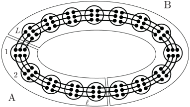
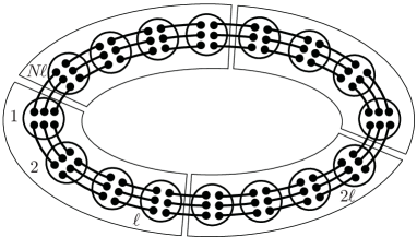
Figure 1: Schematic pictures of the entanglement entropies (left) and the geometric entanglement (right) for the $q$-AKLT model with $S=3$.

Besides the entanglement entropies which characterize the bipartite entanglement, we also study the geometric entanglement, which is another kind of measure for entanglement, see Fig. 1. The geometric entanglement has been proposed as a measure for multipartite entanglement. It has been used to study quantum phase transitions [25, 26, 27, 28, 29, 30, 34, 38, 39], and has been measured experimentally recently [41]. Systems near criticality exhibit logarithmic divergences as the entanglement entropies. On the other hand, only a few analytic results are known for gapped systems. The geometric entanglement defined below can be regarded as the actual distance between the ground state of the system and the nearest fully separable state in the Hilbert space.

We divide the $L$-site chain into $N$ parties ($L=N\ell$). Consider a pure quantum state of $N$ parties $|\Psi\rangle\in H=\otimes_{i=1}^{N}H^{[i]}$, where $H^{[i]}$ is the space of the $i$th party. The entanglement can be quantified by maximizing the fidelity $|\Lambda|$ between the quantum state $|\Psi{\rangle}$ and all the possible separable and normalized states of $N$ parties $|\Phi{\rangle}=\otimes_{i=1}^{N}|\phi^{[i]}{\rangle}$, $|\phi^{[i]}{\rangle}\in H^{[i]}$,

$$|\Lambda_{\max}|=\max_{|\Phi{\rangle}}|\Lambda|,\qquad\Lambda=\frac{{\langle}\Phi|\Psi{\rangle}}{\sqrt{{\langle}\Psi|\Psi{\rangle}}}.$$ (3)

The logarithm of $|\Lambda_{\max}|$ is taken

$$E(\Psi)=-\operatorname{Log}|\Lambda_{\max}|^{2},$$

such that its value becomes zero when $|\Psi{\rangle}$ is separable or positive otherwise. The geometric entanglement per block is defined as the above quantity per party

$$\mathcal{E}(\ell)=-\lim_{N\to\infty}\frac{E(\Psi)}{N},$$

well defined in the thermodynamic limit. We evaluate the geometric entanglement for the spin $S$ $q$-deformed VBS state $|\Psi{\rangle}$. We obtain the expression of the geometric entanglement for $\ell\to\infty$ and its finite size corrections with help of numerical calculations. For the evaluation of the entanglement entropies and the geometric entanglement, the spectral structure of the transfer matrix of the $q$-VBS state in the matrix product representation [3, 24] will be helpful.

This article is organized as follows. In Section 2, we briefly review the matrix product representation [3, 24] of the VBS ground state of the $q$-AKLT model, which helps us for evaluating the entanglement entropies and the geometric entanglement. In Section 3, the finite-size correction terms of the entanglement entropies from the double scaling limit are calculated by perturbative analysis. We emphasize that the double scaling limits of the entanglement entropies and the leading term of the finite-size correction of the entanglement spectrum have been originally obtained by Santos et al. [32]. But we make Section 3 partially overlap their results so that this article can be self-contained and easy to read. In Section 4, we investigate the geometric entanglement with help of numerical calculations. Section 5 is devoted to the summary of this article.

2 $\boldsymbol{q}$-VBS state

In this section, we briefly review the matrix product representation of the higher-integer-spin $q$-VBS ground state and the spectral structure of the transfer matrix of the $q$-AKLT model [3, 24]. We use the following notations. For a real number $c$ we define its $q$ analogue as

$$[c]=\frac{q^{c}-q^{-c}}{q-q^{-1}}.$$

We also define the $q$-shifted factorial and the $q$-shifted binomial for $n\in\mathbb{Z}_{\geq 0}$ as

$$[n]!=\begin{cases}\displaystyle\prod_{i=1}^{n}[i],&n\in{\mathbb{N}},\\ 1,&n=0,\end{cases}\qquad\left[\begin{array}[]{@{}c@{}}n\\ k\end{array}\right]=\begin{cases}\displaystyle\frac{[n]!}{[n]![n-k]!},&k=0,\dots,n,\\ 0,&\rm otherwise.\end{cases}$$

The $q$-VBS state [3, 24], which is the exact ground state of the $q$-AKLT model (2), is expressed in the following matrix product form

$$|\Psi\rangle=\operatorname{Tr}[g_{1}\star g_{2}\star\cdots\star g_{L-1}\star g_{L}],$$

where $g_{k}$ is an $(S+1)\times(S+1)$ vector-valued matrix acting on the $k$-th site whose element is given by

$$g_{k}(a,b)=(-1)^{S-i}q^{(a+b-S)(S+1)/2}\sqrt{\left[\begin{array}[]{@{}c@{}}S\\ a\end{array}\right]\left[\begin{array}[]{@{}c@{}}S\\ b\end{array}\right][S-a+b]![S+a-b]!}\;|S;b-a\rangle_{k}$$

$$\hphantom{g_{k}(a,b)}{}=:h_{ab}|S;b-a\rangle_{k},\qquad(0\leq a,b\leq S).$$

The symbol $\star$ denotes the product $A\star B=\left\{\sum_{y}|\alpha\rangle_{xy}\otimes|\beta\rangle_{yz}\right\}_{xz}$ for vector-valued matrices $A=\left\{|\alpha\rangle_{xy}\right\}_{xy}$ and $B=\left\{|\beta\rangle_{xy}\right\}_{xy}$.

We define $g_{k}^{\dagger}$ by replacing each ket vector in the matrix $g_{k}$ by its corresponding bra vector:

$$g^{\dagger}_{k}(a,b)=h_{ab}\;{}_{k}\langle S;b-a|.$$

Let us set an $(S+1)^{2}$ dimensional vector space as

$$W=\bigoplus_{0\leq a,b\leq S}{\mathbb{C}}|ab{\rangle\!\rangle},$$

where $\{|ab{\rangle\!\rangle}\;|\;a,b=0,\dots,S\}$ is an orthonormal basis. We define an $(S+1)^{2}\times(S+1)^{2}$ matrix $G$ acting on the space $W$ as

$$G=g^{\dagger}\otimes g,\qquad{\langle\!\langle}ab|G|cd{\rangle\!\rangle}=g^{\dagger}(a,c)g(b,d)=\delta_{a-c,b-d}h_{ac}h_{bd},$$

which plays the role of a transfer matrix.

In [3], the spectral structure of the $G$ matrix was clarified, i.e. the eigenvalues of $G$ are given as

$$\lambda_{n}=(-1)^{n}(\left[S\right]!)^{2}\left[\begin{array}[]{@{}c@{}}2S+1\\ S-n\end{array}\right],\qquad n=0,1,\dots,S,$$

with the degree of degeneracy $2n+1$, and thus the squared norm of the ground state is given as

$$\langle\Psi|\Psi\rangle=\operatorname{Tr}G^{L}=\sum_{0\leq n\leq S}(2n+1)\lambda^{L}_{n}.$$ (4)

The matrix $G$ has the following block diagonal structure since ${\langle\!\langle}ab|G|cd{\rangle\!\rangle}=0$ for $a-b\neq c-d$:

$$G=\bigoplus_{-S\leq j\leq S}G^{(j)},\qquad G^{(j)}\in{\rm End}W_{j},\qquad W_{j}=\bigoplus_{i=\max(0,-j)}^{\min(S,S-j)}{\mathbb{C}}|i,i+j{\rangle\!\rangle}.$$

The size of each block $G^{(j)}$ is $(S-|j|+1)\times(S-|j|+1)$. Each element of $G^{(j)}$ is

$${\langle\!\langle}a,a+j|G^{(j)}|c,c+j{\rangle\!\rangle}=(-1)^{j}q^{(a+c+j-S)(S+1)}\left[S-a+c\right]!\left[S+a-c\right]!$$

$$\hphantom{{\langle\!\langle}a,a+j|G^{(j)}|c,c+j{\rangle\!\rangle}=}{}\times\sqrt{\left[\begin{array}[]{@{}c@{}}S\\ a\end{array}\right]\left[\begin{array}[]{@{}c@{}}S\\ a+j\end{array}\right]\left[\begin{array}[]{@{}c@{}}S\\ c\end{array}\right]\left[\begin{array}[]{@{}c@{}}S\\ c+j\end{array}\right]}.$$

We construct intertwiners among the $2S+1$ blocks $G^{(j)}$ $(j=-S,\dots,S)$. This helps us to construct eigenvectors of each block from another block with a smaller size.

Let us define a family of linear operators $\{I_{j}\}_{1\leq|j|\leq S}$ as

$$I_{j}:\ W_{j}\to W_{j-1}\quad(j>0),$$

$$\hphantom{I_{j}:{}}{}\ {\langle\!\langle}a,a+j-1|I_{j}|c,c+j{\rangle\!\rangle}=\begin{cases}\displaystyle q^{-a}\sqrt{\frac{\left[a+j\right]\left[S-a-j+1\right]}{\left[j\right]\left[S-j+1\right]}},&c=a,\\ \displaystyle-q^{1-a-j}\sqrt{\frac{\left[a\right]\left[S-a+1\right]}{\left[j\right]\left[S-j+1\right]}},&c=a-1,\\ 0,&\rm otherwise,\end{cases}$$

$$\hphantom{I_{j}:{}}{}\ W_{j}\to W_{j+1}\quad(j<0),\qquad{\langle\!\langle}a-j-1,a|I_{j}|c-j,c{\rangle\!\rangle}={\langle\!\langle}a,a-j-1|I_{-j}|c,c-j{\rangle\!\rangle}.$$

By direct calculation, one finds that the matrix $I_{j}$ enjoys the intertwining relation $I_{j}G^{(j)}=G^{(j-1)}I_{j}$ $(1\leq j\leq S)$, $I_{j}G^{(j)}=G^{(j+1)}I_{j}$ $(-S\leq j\leq-1)$. Each block $G^{(j)}$ has a simple (nondegenerated) spectrum

$$\operatorname{Spec}G^{(j)}=\{\lambda_{\ell}\}_{|j|\leq\ell\leq S},$$

and the corresponding eigenvectors are given by

$$|\lambda_{n}{\rangle\!\rangle}_{j}=\begin{cases}\displaystyle\sum_{0\leq i\leq S-n}q^{(n+1)i}\sqrt{\frac{\left[S-n\right]!\left[i+n\right]!\left[S-i\right]!}{[S]![n]![S-i-n]![i]!}}|i,i+n{\rangle\!\rangle},&n=j\geq 0,\\ \displaystyle\sum_{0\leq i\leq S-n}q^{(n+1)i}\sqrt{\frac{\left[S-n\right]!\left[i+n\right]!\left[S-i\right]!}{[S]![n]![S-i-n]![i]!}}|i+n,i{\rangle\!\rangle},&-n=j<0,\\ \displaystyle I_{j+1}I_{j+2}\cdots I_{n}|\lambda_{n}{\rangle\!\rangle}_{n},&1\leq j+1\leq n\leq S,\\ I_{j-1}I_{j-2}\cdots I_{-n}|\lambda_{n}{\rangle\!\rangle}_{-n},&1<-j+1\leq n\leq S.\end{cases}$$ (5)

The $\ell$th-power of the $G$ matrix is formally expanded as

$$G^{\ell}=\bigoplus_{-S\leq j\leq S}\sum_{|j|\leq n\leq S}\frac{\lambda_{n}^{\ell}}{{\ \!}_{j}{\langle\!\langle}\lambda_{n}|\lambda_{n}{\rangle\!\rangle}{\ \!\!}_{j}}|\lambda_{n}{\rangle\!\rangle}{\ \!\!}_{j}{\ \!}_{j}{\langle\!\langle}\lambda_{n}|.$$

3 Finite size correction of the entanglement entropies

In this section, we examine the finite-size correction of the entanglement entropies by studying the reduced density matrix. Recently, the following simple formula for the reduced density matrix (1) was found [33]

$$\rho(L,\ell)=\frac{K(L-\ell)K(\ell)}{\operatorname{Tr}G^{L}},$$ (6)

where the “$K$ matrix” is defined as

$$K(\ell)=\mathcal{M}G^{\ell}$$

with a linear map $\mathcal{M}$

$$\mathcal{M}\left(|ab{\rangle\!\rangle}{\langle\!\langle}cd|\right)=|ac{\rangle\!\rangle}{\langle\!\langle}bd|.$$ (7)

The reduced density matrix (6) is an $(S+1)^{2}\times(S+1)^{2}$ matrix, from which the rank of the density matrix is equal to or smaller than $(S+1)^{2}$. We study the reduced density matrix by combining (6) and the spectral structure of the transfer matrix $G$ reviewed in the last section.

Here we introduce some notations and make some general remarks. We define

$$K_{n}=\sum_{-n\leq j\leq n}\frac{1}{{\ \!}_{j}{\langle\!\langle}\lambda_{n}|\lambda_{n}{\rangle\!\rangle}{\ \!\!}_{j}}\mathcal{M}\left(|\lambda_{n}{\rangle\!\rangle}{\ \!\!}_{j}{\ \!}_{j}{\langle\!\langle}\lambda_{n}|\right),$$

so that the $K$ matrix and the reduced density matrix are written as

$$K(\ell)=\sum_{0\leq n\leq S}\lambda_{n}^{\ell}K_{n},$$

$$\rho(L,\ell)=\frac{1}{\sum\limits_{0\leq n\leq S}(2n+1)\lambda^{L}_{n}}\sum_{0\leq n\leq S\atop 0\leq n^{\prime}\leq S}\lambda_{n^{\prime}}^{L-\ell}\lambda_{n}^{\ell}K_{n^{\prime}}K_{n}.$$ (8)

One observes that $K_{n}$, $K(\ell)$ and $\rho(L,\ell)$ enjoy the same block diagonal structure as $G$:

$$K_{n}=\bigoplus_{-S\leq j\leq S}K_{n}^{(j)},\qquad K(\ell)=\bigoplus_{-S\leq j\leq S}K^{(j)}(\ell),\qquad\rho(L,\ell)=\bigoplus_{-S\leq j\leq S}\rho^{(j)}(L,\ell),$$

$$K_{n}^{(j)},K^{(j)}(\ell),\rho^{(j)}(L,\ell)\in\operatorname{End}W_{j},$$

since ${\langle\!\langle}ab|K_{n}|cd{\rangle\!\rangle}=0$ for $a-b\neq c-d$. Note that $\mathcal{M}$ (7) does not always map a matrix acting on a sector $W_{j}$ to a matrix acting on the same sector. The spectrum of $\rho(L,\ell)$ is, of course, given by the union of the spectra of $\rho^{(j)}(L,\ell)$’s. Due to the symmetry ${\langle\!\langle}ab|\rho(L,\ell)|cd{\rangle\!\rangle}={\langle\!\langle}ba|\rho(L,\ell)|dc{\rangle\!\rangle}$, we have the degeneracy

$$\operatorname{Spec}\rho^{(j)}(L,\ell)=\operatorname{Spec}\rho^{(-j)}(L,\ell).$$

3.1 Double scaling limit

We first review the double scaling limit [32, 33]

$$\rho=\lim_{\ell\to\infty}\lim_{L\to\infty}\rho(L,\ell),\qquad\rho^{(i)}=\lim_{\ell\to\infty}\lim_{L\to\infty}\rho^{(i)}(L,\ell).$$

Noting the form (8) and $|\lambda_{n}/\lambda_{0}|<1$ $(n=1,\dots,S)$, we find the reduced density matrix becomes diagonal

$$\rho=K_{0}K_{0},\qquad{\langle\!\langle}ab|\rho|cd{\rangle\!\rangle}=\delta_{ac}\delta_{bd}\frac{q^{2(a+b-S)}}{[S+1]^{2}}\qquad(=:\delta_{ac}\delta_{bd}p_{ab}).$$ (9)

The entanglement spectrum is, of course, given by the diagonal elements of $\rho$, i.e. $\{p_{ab}|a,b=0,1,\dots,S\}$. We notice that the degree of the degeneracy of the eigenvalue $\frac{q^{2k}}{[S+1]^{2}}$ is $S-|k|+1$. For example, the spectrum for $S=2$ is given as

$$\operatorname{Spec}\rho^{(2)}:\quad p_{02}=\frac{1}{[3]^{2}},\qquad$$

$$\operatorname{Spec}\rho^{(1)}:\quad p_{01}=\frac{1}{q^{2}[3]^{2}},\qquad p_{12}=\frac{q^{2}}{[3]^{2}},\quad$$

$$\operatorname{Spec}\rho^{(0)}:\quad p_{00}=\frac{1}{q^{4}[3]^{2}},\qquad p_{11}=\frac{1}{[3]^{2}},\qquad p_{22}=\frac{q^{4}}{[3]^{2}},$$

$$\operatorname{Spec}\rho^{(-1)}:\quad p_{10}=\frac{1}{q^{2}[3]^{2}},\qquad p_{21}=\frac{q^{2}}{[3]^{2}},\quad$$

$$\operatorname{Spec}\rho^{(-2)}:\quad p_{20}=\frac{1}{[3]^{2}}.\qquad$$ (10)

One can calculate

$$P:=\operatorname{Tr}\rho^{\alpha}=\sum_{0\leq a\leq S\atop 0\leq b\leq S}p_{ab}^{\alpha}=\left(\frac{[\alpha(S+1)]}{[\alpha][S+1]^{\alpha}}\right)^{2}.$$ (11)

Then we achieve the entanglement entropies in the double scaling limit [32, 33]

$$S_{\rm R}=\frac{1}{1-\alpha}\operatorname{Log}P=\frac{2}{1-\alpha}\operatorname{Log}\frac{[\alpha(S+1)]}{[\alpha][S+1]^{\alpha}},$$

$$S_{\rm vN}=2\operatorname{Log}q\left(\frac{q+q^{-1}}{q-q^{-1}}-(S+1)\frac{q^{S+1}+q^{-(S+1)}}{q^{S+1}-q^{-(S+1)}}\right)+2\operatorname{Log}[S+1],$$ (12)

see Fig. 2 for the von Neumann entropy in the double scaling limit. In particular, when $q=1$, the spectrum is totally degenerated

$$p_{ab}=\frac{1}{(S+1)^{2}},$$ (13)

and the entropies become

$$S_{\rm R}=S_{\rm vN}=2\operatorname{Log}(S+1),$$

which agree with the case of the open boundary condition [16, 22, 40]. On the other hand, in the limit $q\to 0$, only one eigenvalue survives $p_{00}=1$, $p_{ab}=0$ $(a+b>0)$, and the entropies become zero.

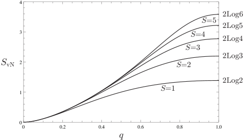
Figure 2: The von Neumann entropy in the double scaling limit $S_{\rm vN}$ (12).

3.2 Finite-size correction

We examine the finite-size correction of the entanglement entropies. We first take the limit $L\to\infty$

$$\rho(\ell):=\lim_{L\to\infty}\rho(L,\ell)=K_{0}\sum_{0\leq n\leq S}K_{n}\kappa_{n}^{\ell},$$ (14)

$$\rho^{(j)}(\ell):=\lim_{L\to\infty}\rho^{(j)}(L,\ell)=K^{(j)}_{0}\sum_{0\leq n\leq S}K^{(j)}_{n}\kappa_{n}^{\ell},$$ (15)

with $\kappa_{n}=\frac{\lambda_{n}}{\lambda_{0}}$, and then consider the case $\ell=1$ and the behavior of the entropies for $\ell\to\infty$. Fig. 3 provides plots of the spectrum $\operatorname{Spec}\rho(\ell)$ of the reduced density matrix (14), i.e. the union of the spectra $\operatorname{Spec}\rho^{(j)}(\ell)$’s of (15), and the von Neumann entropy for $S=2$ with $q=4/5$.

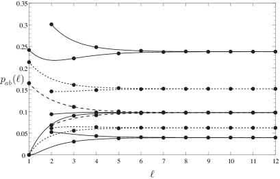
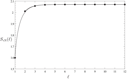
Figure 3: The entanglement spectrum of $\rho(\ell)$ (left) and the von Neumann entropy (right) for $S=2$ with $q=4/5$. The lines are drawn for $\ell\in\mathbb{R}$ with replacement $\kappa_{n}^{\ell}\to|\kappa_{n}|^{\ell}$ and $\kappa_{n}^{\ell}\to\kappa_{n}|\kappa_{n}|^{\ell-1}$ in (14) or (15). In the left figure, the dashed, dotted and solid lines correspond to $\operatorname{Spec}\rho^{(\pm 2)}(\ell)$, $\operatorname{Spec}\rho^{(\pm 1)}(\ell)$ and $\operatorname{Spec}\rho^{(0)}(\ell)$, respectively.

For $\ell=1$ and $L\to\infty$ the reduced density matrix becomes

$$\rho(1)=K_{0}(\mathcal{M}G)/\lambda_{0}.$$

The eigenvalues of $\rho(1)$ become zero except $2S+1$ ones, which is pointed out for $S=1$ and 2 in [32, 33]

$$p_{ab}(1)=\begin{cases}\displaystyle\delta_{a+b,k}\frac{[S+|k|]![S-|k|]!}{[2S+1]!}\sum_{c=0}^{S-|k|}q^{(S+2)(2c+|k|-S)}\left[\begin{array}[]{@{}c@{}}S\\ c\end{array}\right]\left[\begin{array}[]{@{}c@{}}S\\ c+|k|\end{array}\right],&a\times b=0,\\ 0,&{\rm otherwise}.\end{cases}$$ (16)

For example, the spectrum $\{p_{ab}(1)\}_{ab}$ of $\rho(1)$ for $S=2$ is given as

$$\operatorname{Spec}\rho^{(2)}(1):\quad p_{02}(1)=\frac{1}{[5]},\qquad$$

$$\operatorname{Spec}\rho^{(1)}(1):\quad p_{01}(1)=\frac{1+q^{8}}{q^{2}(1+q^{4})[5]},\qquad p_{12}(1)=0,$$

$$\operatorname{Spec}\rho^{(0)}(1):\quad p_{00}(1)=\frac{1-q^{2}+2q^{6}-q^{10}+q^{12}}{q^{4}(1+q^{4})[5]},\qquad p_{11}(1)=0,\qquad p_{22}(1)=0,$$

$$\operatorname{Spec}\rho^{(-1)}(1):\quad p_{10}(1)=\frac{1+q^{8}}{q^{2}\left(1+q^{4}\right)[5]},\qquad p_{21}(1)=0,\qquad$$

$$\operatorname{Spec}\rho^{(-2)}(1):\quad p_{20}(1)=\frac{1}{[5]}.\qquad$$

Let us show (16). We consider the submatrix $\rho^{(k)}(1)$, $k\geq 0$. The case for $k<0$ is similar. By direct calculation, we find the matrix elements of $(S-k+1)\times(S-k+1)$ submatrix $\rho^{(k)}(1)$ are given by

$${\langle\!\langle}c,c+k|\rho^{(k)}(1)|c+j,c+j+k{\rangle\!\rangle}=(-1)^{j}q^{2c+k-S+(2c+j+k-S)(S+1)}\frac{\left[S+k\right]!\left[S-k\right]!}{[2S+1]!}$$

$$\hphantom{{\langle\!\langle}c,c+k|\rho^{(k)}(1)|c+j,c+j+k{\rangle\!\rangle}=}{}\times\sqrt{\left[\begin{array}[]{@{}c@{}}S\\ c\end{array}\right]\left[\begin{array}[]{@{}c@{}}S\\ c+j\end{array}\right]\left[\begin{array}[]{@{}c@{}}S\\ c+k\end{array}\right]\left[\begin{array}[]{@{}c@{}}S\\ c+j+k\end{array}\right]}.$$ (25)

The rank of $\rho^{(k)}(1)$ is 1, since the element of $\rho^{(k)}(1)$ (25) has a form $A_{c}\times B_{c+j}$. Thus, only one eigenvalue of $\rho^{(k)}(1)$ is nonzero, which is given by

$$\operatorname{Tr}_{(k)}\rho^{(k)}(1)=\sum_{c=0}^{S-k}{\langle\!\langle}c,c+k|\rho^{(k)}(1)|c,c+k{\rangle\!\rangle}$$

$$\hphantom{\operatorname{Tr}_{(k)}\rho^{(k)}(1)}{}=\frac{[S+k]![S-k]!}{[2S+1]!}\sum_{c=0}^{S-k}q^{(S+2)(2c+k-S)}\left[\begin{array}[]{@{}c@{}}S\\ c\end{array}\right]\left[\begin{array}[]{@{}c@{}}S\\ c+k\end{array}\right],$$ (30)

from the fact that the other eigenvalues are all 0. The expression (30) is actually identical to the one point functions derived in [3]. In particular, when $q=1$, the non-zero eigenvalues are degenerated as $p_{ab}(1)=\frac{1}{2S+1}$ $(a\times b=0)$, and we have $S_{\rm R}(1)=S_{\rm vN}(1)=\operatorname{Log}(2S+1)$ [32]. One observes the monotonicity of the von Neumann entropy $S_{\rm vN}(1)$ while $0<q<1$, see Fig. 4.

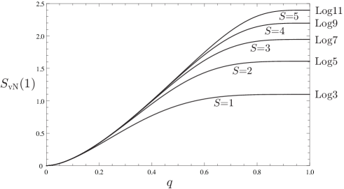
Figure 4: The von Neumann entropy of the one-site subsystem $S_{\rm vN}(1)$.

We turn to the behavior of entropies for $\ell\to\infty$. Noting again the form (8) and $|\kappa_{n}|<1$ $(n=1,\dots,S)$, we find

$$\rho(\ell)=\rho+\kappa_{1}^{\ell}K_{0}K_{1}+O\big{(}\kappa_{2}^{\ell}\big{)},\qquad\ell\to\infty.$$

We denote the eigenvalue of $\rho(\ell)$ by $p_{ab}(\ell)$ corresponding to $p_{ab}$ (9) when $\ell\to\infty$. Since the density matrix $\rho$ in the double scaling limit is a diagonal matrix, it is not difficult to perform perturbative calculation. Noting $|\kappa_{1}|^{2}>|\kappa_{2}|>|\kappa_{3}|>\cdots$, we find

$$p_{ab}(\ell)=p_{ab}+r_{ab}\kappa_{1}^{\ell}+t_{ab}\kappa_{1}^{2\ell}+o\big{(}\kappa_{1}^{2\ell}\big{)},\qquad\ell\to\infty,$$ (31)

$$r_{ab}={\langle\!\langle}ab|K_{0}K_{1}|ab{\rangle\!\rangle},\qquad t_{ab}=\sum_{(c,d)\neq(a,b)\atop 0\leq c,d\leq S}\frac{{\langle\!\langle}cd|K_{0}K_{1}|ab{\rangle\!\rangle}{\langle\!\langle}ab|K_{0}K_{1}|cd{\rangle\!\rangle}}{p_{ab}-p_{cd}}.$$

Inserting (5) into $r_{ab}$ and $t_{ab}$ defined above, we have

$$r_{ab}=\frac{q^{a+b-S}}{[S+1]}\frac{q^{a+b-3S}[3](1-q^{2a}-q^{2a+2}+q^{2S+2})(1-q^{2b}-q^{2b+2}+q^{2S+2})}{(q^{2}-1)^{2}[S][S+1][S+2]},$$ (32)

$$t_{ab}=\left(\frac{q^{2(a+b-S)}[3][2]}{[S+2][S+1][S]}\right)^{2}$$

$$\hphantom{t_{ab}=}{}\times\frac{q^{-4}[S-a+1][a][S-b+1][b]-q^{4}[S-a][a+1][S-b][b+1]}{q^{2}-q^{-2}}.$$ (33)

The first-order term (32) has been originally obtained in [32] (see equation (59) of [32] by changing the indices $\mu=S/2-a$, $\nu=S/2-b$ and redefining $q\to q^{1/2}$), where the characteristic length is given by $\xi=\frac{1}{\operatorname{Log}([S+2]/[S])}$. We also calculated the second-order term (33) which is needed for seeing the finite-size correction of the von Neumann entropy.

For example, the spectrum $\{p_{ab}(\ell)\}_{ab}$ ($\ell\to\infty$) for $S=2$ (which is shifted from (10) as (31)) is given as

$$\operatorname{Spec}\rho^{(2)}(\ell):\quad \frac{1}{[3]^{2}}-\frac{[2]}{[3][4]}\kappa_{1}^{\ell},$$

$$\operatorname{Spec}\rho^{(1)}(\ell):\quad \frac{1}{q^{2}[3]^{2}}+\frac{(1-q^{2})[2]}{q^{2}[3][4]}\kappa_{1}^{\ell}+\frac{q^{2}[2]^{2}}{(1-q^{4})[4]^{2}}\kappa_{1}^{2\ell},$$

$$\frac{q^{2}}{[3]^{2}}-\frac{(1-q^{2})[2]}{[3][4]}\kappa_{1}^{\ell}-\frac{q^{2}[2]^{2}}{(1-q^{4})[4]^{2}}\kappa_{1}^{2\ell},$$

$$\operatorname{Spec}\rho^{(0)}(\ell):\quad \frac{1}{q^{4}[3]^{2}}+\frac{[2]}{q^{2}[3][4]}\kappa_{1}^{\ell}+\frac{[2]^{2}}{q^{2}(1-q^{4})[4]^{2}}\kappa_{1}^{2\ell},$$

$$\frac{1}{[3]^{2}}+\frac{(1-q^{2})^{2}[2]}{q^{2}[3][4]}\kappa_{1}^{\ell}-\frac{[2]}{[4]}\kappa_{1}^{2\ell},\qquad\frac{q^{4}}{[3]^{2}}+\frac{q^{2}[2]}{[3][4]}\kappa_{1}^{\ell}-\frac{q^{6}[2]^{2}}{(1-q^{4})[4]^{2}}\kappa_{1}^{2\ell},$$

$$\operatorname{Spec}\rho^{(-1)}(\ell):\quad \frac{1}{q^{2}[3]^{2}}+\frac{(1-q^{2})[2]}{q^{2}[3][4]}\kappa_{1}^{\ell}+\frac{q^{2}[2]^{2}}{(1-q^{4})[4]^{2}}\kappa_{1}^{2\ell},$$

$$\frac{q^{2}}{[3]^{2}}-\frac{(1-q^{2})[2]}{[3][4]}\kappa_{1}^{\ell}-\frac{q^{2}[2]^{2}}{(1-q^{4})[4]^{2}}\kappa_{1}^{2\ell},$$

$$\operatorname{Spec}\rho^{(-2)}(\ell):\quad \frac{1}{[3]^{2}}-\frac{[2]}{[3][4]}\kappa_{1}^{\ell},$$

where we omit the symbol $+o\big{(}\kappa_{1}^{2\ell}\big{)}$.

The Rényi entropy is expressed by $p_{ab}$, $r_{ab}$ and $t_{ab}$ up to the order of $\kappa_{1}^{2\ell}$ as

$$S_{\rm R}(\ell)=\frac{1}{1-\alpha}\operatorname{Log}\operatorname{Tr}\left(\rho(\ell)\right)^{\alpha}=\frac{1}{1-\alpha}\operatorname{Log}\sum_{0\leq a\leq S\atop 0\leq b\leq S}\left(p_{ab}(\ell)\right)^{\alpha}$$

$$\hphantom{S_{\rm R}(\ell)}{}=\frac{1}{1-\alpha}\operatorname{Log}\big{\{}P\big{(}1+R\kappa^{\ell}_{1}+T\kappa_{1}^{2\ell}\big{)}+o\big{(}\kappa_{1}^{2\ell}\big{)}\big{\}}$$

$$\hphantom{S_{\rm R}(\ell)}{}=S_{\rm R}+\frac{R}{1-\alpha}\kappa^{\ell}_{1}+\frac{1}{1-\alpha}\left(T-\frac{R^{2}}{2}\right)\kappa_{1}^{2\ell}+o\big{(}\kappa_{1}^{2\ell}\big{)},\qquad\ell\to\infty,$$ (34)

where

$$R=\frac{\alpha}{P}\sum_{0\leq a\leq S\atop 0\leq b\leq S}p_{ab}^{\alpha-1}r_{ab},\qquad T=\frac{\alpha}{P}\sum_{0\leq a\leq S\atop 0\leq b\leq S}\left(p_{ab}^{\alpha-1}t_{ab}+\frac{\alpha-1}{2}p_{ab}^{\alpha-2}r_{ab}^{2}\right),$$

with $P$ defined by (11).

By tedious but straightforward calculation, one finds

$$R=\frac{\alpha[3]}{[S][S+2]}\left(\frac{[S+2][\alpha S]-[\alpha(S+2)][S]}{(q-q^{-1})[\alpha(S+1)][\alpha+1]}\right)^{2},$$

$$T=\alpha\left(\frac{[2][3]}{(q-q^{-1})^{2}[S][S+2]}\right)^{2}\left[\frac{[2(\alpha-1)]}{[2]}\left(\frac{([(S+2)(\alpha+1)][S]-[S+2][S(\alpha+1)])}{[\alpha+2][\alpha+1][\alpha(S+1)]}\right)^{2}\right.$$

$$\left.\hphantom{T=}{}+\frac{\alpha-1}{2}\left(\frac{[2(S+1)]^{2}}{[2][S+1]^{2}}-\frac{2[2(S+1)][\alpha][(\alpha+1)(S+1)]}{[S+1][\alpha(S+1)][\alpha+1]}+\frac{[2][\alpha][(\alpha+2)(S+1)]}{[(S+1)\alpha][\alpha+2]}\right)^{2}\right].$$

Then we find

$$S_{\rm vN}(\ell)=S_{\rm vN}+\left(\frac{4q^{2}\operatorname{Log}q}{1-q^{4}}-\frac{1}{2}\right)\kappa_{1}^{2\ell}+o\big{(}\kappa_{1}^{2\ell}\big{)},\qquad\ell\to\infty,$$ (35)

where the coefficient of $\kappa_{1}^{\ell}$ vanishes. Since the leading order term is $\kappa_{1}^{2\ell}$, the characteristic length is $2\xi$. We find the coefficient of $\kappa_{1}^{2\ell}$ depends on the anisotropy parameter $q$ but is independent of the spin value $S$.

As discussed in [32], the perturbation fails for the isotropic case due to the degeneracy (13), but the entanglement spectrum can be written by linear combinations of $\kappa_{n}$’s and has the same spectral structure for the transfer matrix $G$. For example, for $S=2$, we have

$$\operatorname{Spec}\rho^{(2)}(\ell):\quad \frac{1}{3}\left(\frac{1}{3}-\frac{\kappa_{1}^{\ell}}{2}+\frac{\kappa_{2}^{\ell}}{6}\right),\qquad$$

$$\operatorname{Spec}\rho^{(1)}(\ell):\quad \frac{1}{3}\left(\frac{1}{3}-\frac{\kappa_{1}^{\ell}}{2}+\frac{\kappa_{2}^{\ell}}{6}\right),\qquad \frac{1}{3}\left(\frac{1}{3}+\frac{\kappa_{1}^{\ell}}{2}-\frac{5\kappa_{2}^{\ell}}{6}\right),\qquad$$

$$\operatorname{Spec}\rho^{(0)}(\ell):\quad \frac{1}{3}\left(\frac{1}{3}-\frac{\kappa_{1}^{\ell}}{2}+\frac{\kappa_{2}^{\ell}}{6}\right),\qquad \frac{1}{3}\left(\frac{1}{3}+\frac{\kappa_{1}^{\ell}}{2}-\frac{5\kappa_{2}^{\ell}}{6}\right),\qquad \frac{1}{3}\left(\frac{1}{3}+\kappa_{1}^{\ell}+\frac{5\kappa_{2}^{\ell}}{3}\right),$$

$$\operatorname{Spec}\rho^{(-1)}(\ell):\quad \frac{1}{3}\left(\frac{1}{3}-\frac{\kappa_{1}^{\ell}}{2}+\frac{\kappa_{2}^{\ell}}{6}\right),\qquad \frac{1}{3}\left(\frac{1}{3}+\frac{\kappa_{1}^{\ell}}{2}-\frac{5\kappa_{2}^{\ell}}{6}\right),$$

$$\operatorname{Spec}\rho^{(-2)}(\ell):\quad \frac{1}{3}\left(\frac{1}{3}-\frac{\kappa_{1}^{\ell}}{2}+\frac{\kappa_{2}^{\ell}}{6}\right),\qquad$$

where no higher order term is needed. In [32] the finite-size corrections of the entanglement entropies for $q=1$ were calculated as

$$S_{\rm R}(\ell)=2\operatorname{Log}(S+1)-\frac{3}{2}\alpha\kappa_{1}^{2\ell}+o\big{(}\kappa_{1}^{2\ell}\big{)},\qquad\ell\to\infty,$$

$$S_{\rm vN}(\ell)=2\operatorname{Log}(S+1)-\frac{3}{2}\kappa_{1}^{2\ell}+o\big{(}\kappa_{1}^{2\ell}\big{)},\qquad\ell\to\infty,$$

which agree with the limits $q\to 1$ of (34) and (35).

4 Geometric entanglement

In this section, we evaluate the geometric entanglement, which is another kind of measure of entanglement. We divide the chain into $N$ parties ($L=N\ell$), and each of the $N$ parties to be contiguous blocks of $\ell$ spins $S$. When $N$ is large enough, the following expression for the fidelity $|\Lambda_{\max}|$ (3) has been shown for $PT$-symmetric matrix product ground states $|\Psi{\rangle}$ in [25, 26, 29]

$$|\Lambda_{\max}|^{2}=\lim_{N\to\infty}\frac{|d|^{2N}}{{\langle}\Psi|\Psi{\rangle}},$$ (36)

where $|d|^{2}$ is the quantity

$$|d|^{2}=\max_{\{x_{i}\}:\,\sum\limits_{i=0}^{S}|x_{i}|^{2}=1}{\langle}\operatorname{Aux}|G^{\ell}|\operatorname{Aux}{\rangle},\qquad|\operatorname{Aux}{\rangle}=\sum_{0\leq a\leq S\atop 0\leq b\leq S}x_{a}x_{b}^{*}|ab{\rangle\!\rangle}.$$ (37)

Performing the maximization (37), one obtains the fidelity $|\Lambda_{\max}|$ which finally leads to the analytic expression for the geometric entanglement $\mathcal{E}(\ell)$

$$\mathcal{E}(\ell)=-\lim_{N\to\infty}\frac{\operatorname{Log}|\Lambda_{\max}|^{2}}{N}.$$

For convenience we set $x_{i}=r_{i}e^{\sqrt{-1}\theta_{i}}$ ($r_{i}\geq 0$, $\theta_{i}\in\mathbb{R}$), and write $x^{\bullet}_{i}=r^{\bullet}_{i}e^{\sqrt{-1}\theta^{\bullet}_{i}}$ if the setting $\{x_{i}=x^{\bullet}_{i}\}$ maximizes $\langle\operatorname{Aux}|G^{\ell}|\operatorname{Aux}\rangle$.

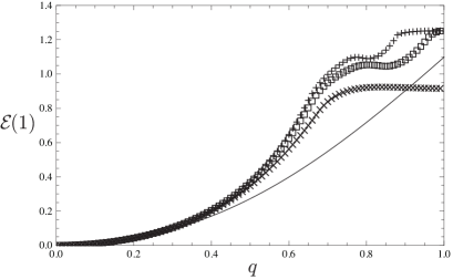
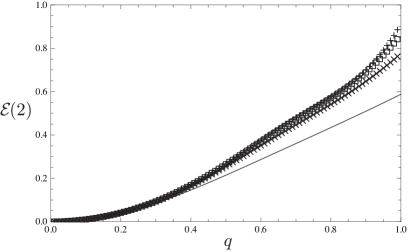
Figure 5: The geometric entanglements for $\ell=1$ (left) and 2 (right). In each graph, the line corresponds to $S=1$ (38), and the markers $\times$ ($S=2$), $\square$ ($S=3$) and $+$ ($S=4$) are plotted based on numerical calculations.

4.1 Spin-1

We calculate the geometric entanglement for $S=1$. By direct calculation, we have

$${\langle}\operatorname{Aux}|G^{\ell}|\operatorname{Aux}{\rangle}=\left(\frac{[3]^{\ell}}{q[2]}+\frac{(-1)^{\ell}}{q^{-1}[2]}\right)|x_{0}|^{4}+\left(\frac{2[3]^{\ell}}{[2]}+2(-1)^{\ell}-\frac{2(-1)^{\ell}}{[2]}\right)|x_{0}|^{2}|x_{1}|^{2}$$

$$\hphantom{{\langle}\operatorname{Aux}|G^{\ell}|\operatorname{Aux}{\rangle}=}{}+\left(\frac{q[3]^{\ell}}{[2]}+\frac{q^{-1}(-1)^{\ell}}{[2]}\right)|x_{1}|^{4}.$$

Inserting $r_{1}^{2}=1-r_{0}^{2}$, we get

$${\langle}\operatorname{Aux}|G^{\ell}|\operatorname{Aux}{\rangle}=\frac{1-q}{1+q^{2}}\big{(}[3]^{\ell}-(-1)^{\ell}\big{)}\left((1-q)r_{0}^{4}+2qr_{0}^{2}\right)+\frac{q^{2}[3]^{\ell}}{1+q^{2}}+\frac{(-1)^{\ell}}{1+q^{2}},$$

where $\theta_{i}$’s do not appear. Thus we find

$$0<q<1:\quad r_{0}^{\bullet}=1,\qquad|d|^{2}=\frac{[3]^{\ell}}{1+q^{2}}+\frac{q^{2}(-1)^{\ell}}{1+q^{2}},$$

$$q=1:\quad |d|^{2}=\frac{3^{\ell}}{2}+\frac{(-1)^{\ell}}{2},$$

$$q>1:\quad r_{0}^{\bullet}=0,\qquad|d|^{2}=\frac{q^{2}[3]^{\ell}}{1+q^{2}}+\frac{(-1)^{\ell}}{1+q^{2}},$$ (38)

where $|d|^{2}={\langle}\operatorname{Aux}|G^{\ell}|\operatorname{Aux}{\rangle}$ is independent of $\{x_{i}\}$ at the isotropic point $q=1$ [25], and the choice of $r^{{\bullet}}_{0}$ changes discontinuously at this point. (We will see that this kind of “degeneracy” occurs for the higher spin case.) Inserting these forms and ${\langle}\Psi|\Psi{\rangle}=[3]^{L}+3(-1)^{L}$ into (36), we finally achieve the geometric entanglement

$$0<q<1:\quad \mathcal{E}(\ell)=\operatorname{Log}\big{(}1+q^{2}\big{)}-\operatorname{Log}\big{(}1+q^{2}(-[3])^{-\ell}\big{)},$$

$$q=1:\quad \mathcal{E}(\ell)=\operatorname{Log}2-\operatorname{Log}\big{(}1+(-[3])^{-\ell}\big{)},$$

$$q>1:\quad \mathcal{E}(\ell)=\operatorname{Log}\big{(}1+q^{2}\big{)}-\operatorname{Log}\big{(}q^{2}+(-[3])^{-\ell}\big{)},$$

which generalizes [25]. The entanglement entropy takes its maximum at the isotropic point, decreases with the decrease of the anisotropy parameter $q$ and finally becomes $\mathcal{E}(\ell)=0$ at $q=0$, see Fig. 5. This behavior of the geometric entanglement is similar to the entanglement entropies. In the limit $\ell\to\infty$, we have

$$\mathcal{E}=\operatorname{Log}\big{(}1+q^{2}\big{)}.$$

4.2 Spin-2

Let us consider first the isotropic case, where we have

$${\langle}\operatorname{Aux}|G^{\ell}|\operatorname{Aux}{\rangle}$$

$$\qquad{}=\frac{1}{3}\lambda_{0}^{\ell}+\frac{1}{2}\lambda_{1}^{\ell}+\frac{1}{6}\lambda_{2}^{\ell}-\frac{(1-(r_{0}-r_{2})^{2})^{2}-4r_{0}r_{1}^{2}r_{2}(\cos(\theta_{0}-2\theta_{1}+\theta_{2})+1)}{2}\big{(}\lambda_{1}^{\ell}-\lambda_{2}^{\ell}\big{)}$$

$$\qquad{}=\frac{1}{3}\lambda_{0}^{\ell}+\frac{1}{2}\lambda_{1}^{\ell}+\frac{1}{6}\lambda_{2}^{\ell}-\frac{(r_{1}^{2}-2r_{0}r_{2})^{2}-4r_{0}r_{1}^{2}r_{2}(\cos(\theta_{0}-2\theta_{1}+\theta_{2})-1)}{2}\big{(}\lambda_{1}^{\ell}-\lambda_{2}^{\ell}\big{)}$$

with $\lambda_{0}=40$, $\lambda_{1}=-20$ and $\lambda_{2}=4$. When $\ell$ is odd (resp. even), $\lambda_{1}^{\ell}<\lambda_{2}^{\ell}$ (resp. $\lambda_{1}^{\ell}>\lambda_{2}^{\ell}$). Using the first (resp. second) form, we find

$$\ell\ {\rm odd}:\quad r_{0}^{{\bullet}}-r_{2}^{\bullet}=0,\qquad\cos(\theta^{\bullet}_{0}-2\theta^{\bullet}_{1}+\theta^{\bullet}_{2})=-1,\qquad|d|^{2}=\frac{1}{3}\lambda_{0}^{\ell}+\frac{2}{3}\lambda_{2}^{\ell},$$

$$\ell\ {\rm even}:\quad r_{1}^{{\bullet}2}-2r_{0}^{\bullet}r_{2}^{\bullet}=0,\qquad\cos(\theta^{\bullet}_{0}-2\theta^{\bullet}_{1}+\theta^{\bullet}_{2})=1,\qquad|d|^{2}=\frac{1}{3}\lambda_{0}^{\ell}+\frac{1}{2}\lambda_{1}^{\ell}+\frac{1}{6}\lambda_{2}^{\ell}.$$

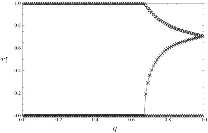
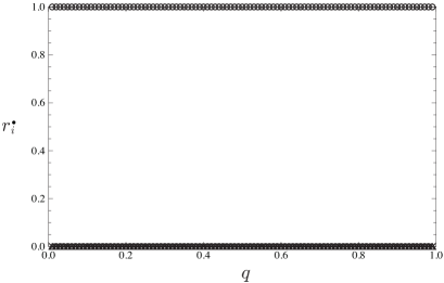
Figure 6: Numerical calculations of the sets $\{r_{i}^{\bullet}\}$ which maximize $|d|^{2}$ for $S=2$ and $\ell=1$ (left) and 2 (right). The markers $\bigcirc$, $\triangle$ and $\times$ correspond to $r_{0}^{\bullet}$, $r_{1}^{\bullet}$ and $r_{2}^{\bullet}$, respectively.

In the anisotropic case, thanks to the form

$$\langle\operatorname{Aux}|G^{\ell}|\operatorname{Aux}\rangle=\frac{4q^{2}r_{0}r_{1}^{2}r_{2}}{1+q^{4}}\big{(}\lambda_{1}^{\ell}-\lambda_{2}^{\ell}\big{)}\cos(\theta_{0}-2\theta_{1}+\theta_{2})+\text{(independent of}\ \{\theta_{i}\}),$$

we have

$$\ell\ {\rm odd}:\quad \cos(\theta^{\bullet}_{0}-2\theta^{\bullet}_{1}+\theta^{\bullet}_{2})=-1,$$

$$\ell\ {\rm even}:\quad \cos(\theta^{\bullet}_{0}-2\theta^{\bullet}_{1}+\theta^{\bullet}_{2})=1,$$

which is the same as for the isotropic case. We use help of numerical calculations (see Fig. 6 for $\ell=1$ and 2), which indicates that

$$\ell\ {\rm odd}:\quad r_{i}^{\bullet}=\delta_{i0}\ {\rm for}\ q\leq\exists\,q^{\bullet};\ r_{0}^{\bullet}>0,\ r_{1}^{\bullet}=0,\ r_{2}^{\bullet}>0\ {\rm for}\ q^{\bullet}<q<1,$$

$$\ell\ {\rm even}:\quad r_{i}^{\bullet}=\delta_{i0}\ \text{always maximizes}\ \langle\operatorname{Aux}|G^{\ell}|\operatorname{Aux}\rangle.$$

One observes that the geometric entanglement with $\ell$ odd is not completely monotonic while $0<q<1$, see Fig. 5. The set $\{r_{0}^{\bullet},r_{2}^{\bullet}\}$ is obtained by

$$\frac{d}{dr_{0}}\left(\langle\operatorname{Aux}|G^{\ell}|\operatorname{Aux}\rangle\big{|}_{r_{1}=0,r_{2}=\sqrt{1-r_{0}^{2}},\cos(\theta_{0}-2\theta_{1}+\theta_{2})=1}\right)=0$$

in the case where $\ell$ is odd and $q^{\bullet}<q<1$

$$r_{0}^{\bullet}=q\sqrt{\frac{-(1-q^{2})(1+q^{4})\lambda_{0}^{\ell}+2[3]\lambda_{1}^{\ell}-(1+3q^{2}+q^{4}+q^{6})\lambda_{2}^{\ell}}{(1-q^{2})^{2}(1+q^{4})\lambda_{0}^{\ell}+4q^{2}[3]\lambda_{1}^{\ell}-(1+2q^{2}+6q^{4}+2q^{6}+q^{8})\lambda_{2}^{\ell}}}.$$ (39)

The transition point $q^{\bullet}$ is obtained by solving (39) $=1$, which approaches 1 as $\ell\to\infty$. The set $\{r_{i}^{\bullet}\}$ for $q>1$ is obtained by replacing $r_{0}\leftrightarrow r_{1}$ and $q\to 1/q$. Under the assumption $r_{i}^{\bullet}=\delta_{i0}$, we have

$$\mathcal{E}(\ell)=-\operatorname{Log}\frac{|d|^{2}}{\lambda_{0}^{\ell}}=-\operatorname{Log}\langle\operatorname{Aux}|G^{\ell}|\operatorname{Aux}\rangle|_{r_{i}=\delta_{i0}}$$

$$\hphantom{\mathcal{E}(\ell)}{}=\operatorname{Log}(1+q^{2}+q^{4})-\operatorname{Log}\left(1+\frac{q^{2}(1+q^{2}+q^{4})\kappa_{1}^{\ell}}{1+q^{4}}+\frac{q^{8}\kappa_{2}^{\ell}}{1+q^{4}}\right),$$

for $0<q<1$ and sufficiently large $\ell$.

4.3 Spin-3

For the isotropic case, we have

$${\langle}\operatorname{Aux}|G^{\ell}|\operatorname{Aux}{\rangle}=\frac{1}{4}\lambda_{0}^{\ell}+\frac{9}{20}\lambda_{1}^{\ell}+\frac{1}{4}\lambda_{2}^{\ell}+\frac{1}{20}\lambda_{3}^{\ell}-\frac{A}{5}(\lambda_{1}^{\ell}-\lambda_{3}^{\ell}),$$

$$A=\Big{[}(r_{1}r_{2}-3r_{0}r_{3})^{2}+2\big{(}r_{2}^{2}-\sqrt{3}r_{1}r_{3}\big{)}^{2}+2\big{(}r_{1}^{2}-\sqrt{3}r_{0}r_{2}\big{)}^{2}$$

$$\hphantom{A=}{}-2r_{1}r_{2}\big{\{}3r_{0}r_{3}(\cos(\alpha+\beta)-1)+2\sqrt{3}r_{0}r_{1}(\cos\alpha-1)+2\sqrt{3}r_{2}r_{3}(\cos\beta-1)\big{\}}\Big{]},$$

where $\alpha=\theta_{0}-2\theta_{1}+\theta_{2}$ and $\beta=\theta_{1}-2\theta_{2}+\theta_{3}$. When $\ell$ is even, $\lambda_{1}^{\ell}>\lambda_{3}^{\ell}$. Thus ${\langle}\operatorname{Aux}|G^{\ell}|\operatorname{Aux}{\rangle}$ is maximized by

$$r_{2}^{{\bullet}2}-\sqrt{3}r^{\bullet}_{1}r^{\bullet}_{3}=r_{1}^{{\bullet}2}-\sqrt{3}r^{\bullet}_{0}r^{\bullet}_{2}=0,\qquad\cos\alpha^{\bullet}=\cos\beta^{\bullet}=1,$$

$$|d|^{2}=\frac{1}{4}\lambda_{0}^{\ell}+\frac{9}{20}\lambda_{1}^{\ell}+\frac{1}{4}\lambda_{2}^{\ell}+\frac{1}{20}\lambda_{3}^{\ell}.$$

When $\ell$ is odd, the candidates of $\{\theta_{i}\}$ that maximize ${\langle}\operatorname{Aux}|G^{\ell}|\operatorname{Aux}{\rangle}$ for given $\{r_{i}\}$ are

$$\cos\alpha=\frac{3r_{2}^{2}r_{3}^{2}-4r_{1}^{2}r_{2}^{2}-3r_{0}^{2}r_{1}^{2}}{4\sqrt{3}r_{0}r_{1}^{2}r_{2}},\qquad\cos\beta=\frac{3r_{0}^{2}r_{1}^{2}-4r_{1}^{2}r_{2}^{2}-3r_{2}^{2}r_{3}^{2}}{4\sqrt{3}r_{1}r_{2}^{2}r_{3}},$$

$$\cos(\alpha+\beta)=-\frac{3r_{0}^{2}r_{1}^{2}-4r_{1}^{2}r_{2}^{2}+3r_{2}^{2}r_{3}^{2}}{6r_{0}r_{1}r_{2}^{2}r_{3}},$$ (40)

$$\text{or}\quad\cos\alpha=-1,\qquad\cos\beta=-1,\qquad\cos(\alpha+\beta)=1,$$ (41)

$$\text{or}\quad\cos\alpha=1,\qquad\cos\beta=-1,\qquad\cos(\alpha+\beta)=-1,$$ (42)

$$\text{or}\quad\cos\alpha=-1,\qquad\cos\beta=1,\qquad\cos(\alpha+\beta)=-1.$$ (43)

Inserting (40), we get

$$A=\frac{9}{4}-\left(3r_{0}^{2}+2r_{1}^{2}+r_{2}^{2}-\frac{3}{2}\right)^{2},$$

and thus we find

$$3r_{0}^{{\bullet}2}+2r_{1}^{{\bullet}2}+r_{2}^{{\bullet}2}=\frac{3}{2},\qquad|d|^{2}=\frac{1}{4}\lambda_{0}^{\ell}+\frac{1}{4}\lambda_{2}^{\ell}+\frac{1}{2}\lambda_{3}^{\ell}.$$ (44)

We end up achieving the same value $|d|^{2}$ (44) for (41)–(43). For example, inserting (41), we get

$$A=\frac{9}{4}-\left(3r_{0}^{2}+2r_{1}^{2}+r_{2}^{2}-\frac{3}{2}\right)^{2}-\big{(}\sqrt{3}r_{0}r_{1}-r_{1}r_{2}+\sqrt{3}r_{2}r_{3}\big{)}^{2}.$$

The maximization for the anisotropic case with $\ell$ odd is more complicated than $S=2$, see the numerical result in Fig. 7. We expect that

$$\ell\ {\rm odd}:\quad \text{there exist}\ q^{\bullet},\ q^{{\bullet}{\bullet}},\ q^{{\bullet}{\bullet}{\bullet}}\ {\rm and}\ q^{{\bullet}{\bullet}{\bullet}{\bullet}}\ \text{such that}$$

$$\begin{cases}r^{\bullet}_{i}=\delta_{i0},&0<q\leq q^{\bullet},\\ r_{1}^{\bullet}=r_{3}^{\bullet}=0,\ r_{0}^{\bullet}>0,\ r_{2}^{\bullet}>0,&q^{\bullet}<q\leq q^{{\bullet}{\bullet}},\\ r_{i}^{\bullet}>0,\ i=0,1,2,3,&q^{{\bullet}{\bullet}}<q<q^{{\bullet}{\bullet}{\bullet}},\\ r_{i}^{\bullet}=\delta_{i1},&q^{{\bullet}{\bullet}{\bullet}}\leq q<q^{{\bullet}{\bullet}{\bullet}{\bullet}},\\ r_{0}^{\bullet}=r_{2}^{\bullet}=0,\ r_{1}^{\bullet}>0,\ r_{3}^{\bullet}>0,&q^{{\bullet}{\bullet}{\bullet}{\bullet}}\leq q<1,\end{cases}$$

$$\ell\ {\rm even}:\quad r_{i}^{\bullet}=\delta_{i0}\ \text{always maximizes}\ \langle\operatorname{Aux}|G^{\ell}|\operatorname{Aux}\rangle.$$

We also expect that these transition points $q^{\bullet},\dots,q^{{\bullet}{\bullet}{\bullet}{\bullet}}$ approach 1 as $\ell\to\infty$. Under the assumption $r_{i}^{\bullet}=\delta_{i0}$, we have

$$\mathcal{E}(\ell)=-\operatorname{Log}\frac{|d|^{2}}{\lambda_{0}^{\ell}}=-\operatorname{Log}\langle\operatorname{Aux}|G^{\ell}|\operatorname{Aux}\rangle|_{r_{i}=\delta_{i0}}$$

$$\hphantom{\mathcal{E}(\ell)}{}=\operatorname{Log}q^{3}[4]-\operatorname{Log}\left(1+\frac{q^{2}[3]^{2}\kappa_{1}^{\ell}}{[5]}+\frac{q^{8}\kappa_{2}^{\ell}}{1-q^{2}+q^{4}}+\frac{q^{14}\kappa_{3}^{\ell}}{(1-q^{2}+q^{4})[5]}\right),$$

for $0<q<1$ and sufficiently large $\ell$.

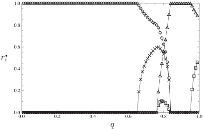
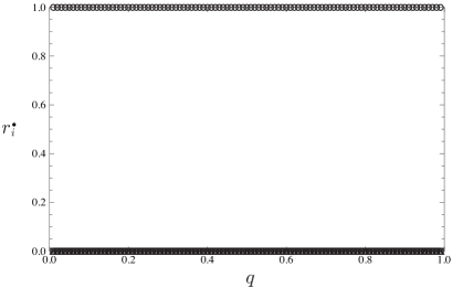
Figure 7: Numerical calculations of the sets $\{r_{i}^{\bullet}\}$ which maximize $|d|^{2}$ for $S=3$ and $\ell=1$ (left) and 2 (right). The markers $\bigcirc$, $\triangle$, $\times$ and $\square$ correspond to $r_{0}^{\bullet}$, $r_{1}^{\bullet}$, $r_{2}^{\bullet}$ and $r_{3}^{\bullet}$, respectively.

4.4 General case

We consider the maximization of $\langle\operatorname{Aux}|G^{\ell}|\operatorname{Aux}\rangle$ for general $S$. As we observed in the previous subsections, we expect that, for given $q<1$,

• $\ell$ odd: there exists $\ell^{\bullet}$ such that the set $\{r^{\bullet}_{i}=\delta_{i0}\}$ maximizes $\langle\operatorname{Aux}|G^{\ell}|\operatorname{Aux}\rangle$ when $\ell>\ell^{\bullet}$,

• $\ell$ even: the set $\{r^{\bullet}_{i}=\delta_{i0}\}$ always maximizes $\langle\operatorname{Aux}|G^{\ell}|\operatorname{Aux}\rangle$.

Since the term $\frac{\lambda_{0}^{\ell}}{{}_{0}{\langle\!\langle}\lambda_{0}|\lambda_{0}{\rangle\!\rangle}_{0}}\left|\sum\limits_{a=0}^{S}q^{a}r_{a}^{2}\right|^{2}$ dominates in $\langle\operatorname{Aux}|G^{\ell}|\operatorname{Aux}\rangle$ for $\ell\to\infty$, we have $r_{i}^{\bullet}\to\delta_{i0}$, which supports the above assumption. Inserting $\{r_{i}=\delta_{i0}\}$, we have

$$|d|^{2}={\langle}\operatorname{Aux}|G^{\ell}|\operatorname{Aux}{\rangle}\Big{|}_{r_{i}=\delta_{i0}}=\sum_{k=0}^{S}\frac{\lambda_{k}^{\ell}}{{}_{0}{\langle\!\langle}\lambda_{k}|\lambda_{k}{\rangle\!\rangle}_{0}},$$

and find

$$\mathcal{E}(\ell)=-\operatorname{Log}\left(\sum_{k=0}^{S}\frac{\kappa_{k}^{\ell}}{{}_{0}{\langle\!\langle}\lambda_{k}|\lambda_{k}{\rangle\!\rangle}_{0}}\right)$$

$$\hphantom{\mathcal{E}(\ell)}{}=\operatorname{Log}(q^{S}[S+1])-\operatorname{Log}\left(\sum_{k=0}^{S}q^{k(k+1)}\frac{[2k+1][S]![S+1]!}{[S+k+1]![S-k]!}\kappa_{k}^{\ell}\right)$$

$$\hphantom{\mathcal{E}(\ell)}{}=\operatorname{Log}(q^{S}[S+1])-\frac{q^{2}[3][S]}{[S+2]}\kappa_{1}^{\ell}+o\big{(}\kappa_{1}^{\ell}\big{)},\qquad\ell\to\infty.$$ (45)

Here we used the norm (4) of the $q$-deformed VBS state $|\Psi\rangle$ and the norm of the eigenvectors of the transfer matrix [3]. In the limit $\ell\to\infty$, we have the geometric entanglement $\mathcal{E}=\operatorname{Log}(q^{S}[S+1])$, which takes the maximum $\operatorname{Log}(S+1)$ at $q=1$ and approaches 0 as $q\to 0$, see Fig. 8. The monotonic behavior while $0<q<1$ is similar to the entanglement entropies.

The isotropic point is a special case where the choice $r_{i}=\delta_{0i}$ or $r_{i}=\delta_{Si}$ does not always maximize $|d|^{2}$ for $S\geq 2$ even if $\ell$ is large, as we saw for $S=2$ and $S=3$. Thus the asymptotic form (45) is no longer valid at the isotropic point.

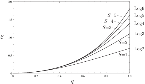
Figure 8: The geometric entanglement in the limit $\ell\to\infty$.

5 Summary and discussion

In this article, we studied some entanglement properties of the higher spin $q$-AKLT model with the periodic boundary condition from the matrix product representation of the $q$-VBS ground state. We exactly calculated the finite-size correction terms of the entanglement entropies by the perturbative calculation for the spectrum of the reduced density matrix. We found that the first-order correction term of the Rényi entropy vanishes by taking the limit $\alpha\to 1$. This requires the second-order perturbation of the entanglement spectrum for calculation of the finite-size correction of the von Neumann entropy. It would be interesting to extend the study of entanglement properties to various generalizations, the entanglement entropies with multiple blocks (see [31] for the isotropic spin-1 case), for example. We also investigated the geometric entanglement. The geometric entanglement in the limit $\ell\to\infty$ decreases with the decrease of the anisotropy parameter $q$ while $0<q<1$. This property is the same as the entanglement entropies. Under an assumption which is based on numerical results, we calculated the finite-size correction of the geometric entanglement.

Acknowledgements

C. Arita is a JSPS Fellow for Research Abroad.

References

- [1] Affleck I., Kennedy T., Lieb E.H., Tasaki H., Valence bond ground states in isotropic quantum antiferromagnets, Comm. Math. Phys. 115 (1988), 477–528.
- [2] Amico L., Fazio R., Osterloh A., Vedral V., Entanglement in many-body systems, Rev. Modern Phys. 80 (2008), 517–576, quant-ph/0703044.
- [3] Arita C., Motegi K., Spin-spin correlation functions of the -valence-bond-solid state of an integer spin model, J. Math. Phys. 52 (2011), 063303, 15 pages, arXiv:1009.4018.
- [4] Arovas D.P., Auerbach A., Haldane F.D.M., Extended Heisenberg models of antiferromagnetism: analogies to the fractional quantum Hall effect, Phys. Rev. Lett. 60 (1988), 531–534.
- [5] Batchelor M.T., Mezincescu L., Nepomechie R.I., Rittenberg V., -deformations of the symmetric spin- Heisenberg chain, J. Phys. A: Math. Gen. 23 (1990), L141–L144.
- [6] Bennett C.H., DiVincenzo D.P., Quantum information and computation, Nature 404 (2000), 247–255.
- [7] Calabrese P., Cardy J., Entanglement entropy and quantum field theory, J. Stat. Mech. Theory Exp. 2004 (2004), P06002, 27 pages, hep-th/0405152.
- [8] Drinfel’d V.G., Hopf algebras and the quantum Yang–Baxter equation, Dokl. Akad. Nauk SSSR 32 (1985), 254–258.
- [9] Fang H., Korepin V.E., Roychowdhury V., Entanglement in a valence-bond-solid state, Phys. Rev. Lett. 93 (2004), 227203, 4 pages, quant-ph/0406067.
- [10] Fannes M., Nachtergaele B., Werner R.F., Exact antiferromagnetic ground-states of quantum spin chains, Europhys. Lett. 10 (1989), 633–637.
- [11] Freitag W.D., Müller-Hartmann E., Complete analysis of two spin correlations of valence bond solid chains for all integer spins, Z. Phys. B 83 (1991), 381–390.
- [12] García-Ripoll J.J., Martín-Delgado M.A., Cirac J.I., Implementation of spin Hamiltonians in optical lattices, Phys. Rev. Lett. 93 (2004), 250405, 4 pages, cond-mat/0404566.
- [13] Haldane F.D.M., Continuum dynamics of the -D Heisenberg antiferromagnet: identification with the nonlinear sigma model, Phys. Lett. A 93 (1983), 464–468.
- [14] Haldane F.D.M., Nonlinear field theory of large-spin Heisenberg antiferromagnets: semiclassically quantized solitons of the one-dimensional easy-axis Néel state, Phys. Rev. Lett. 50 (1983), 1153–1156.
- [15] Jimbo M., A -difference analogue of and the Yang–Baxter equation, Lett. Math. Phys. 10 (1985), 63–69.
- [16] Katsura H., Hirano T., Hatsugai Y., Exact analysis of entanglement in gapped quantum spin chains, Phys. Rev. B 76 (2007), 012401, 4 pages, cond-mat/0702196.
- [17] Katsura H., Hirano T., Korepin V.E., Entanglement in an valence-bond-solid state, J. Phys. A: Math. Theor. 41 (2008), 135304, 13 pages, arXiv:0711.3882.
- [18] Katsura H., Kawashima N., Kirillov A.N., Korepin V.E., Tanaka S., Entanglement in valence-bond-solid states on symmetric graphs, J. Phys. A: Math. Theor. 43 (2010), 255303, 28 pages, arXiv:1003.2007.
- [19] Klümper A., Schadschneider A., Zittartz J., Equivalence and solution of anisotropic spin- models and generalized - fermion models in one dimension, J. Phys. A: Math. Gen. 24 (1991), L955–L959.
- [20] Klümper A., Schadschneider A., Zittartz J., Groundstate properties of a generalized VBS-model, Z. Phys. B 87 (1992), 281–287.
- [21] Klümper A., Schadschneider A., Zittartz J., Matrix product ground states for one-dimensional spin-1 quantum antiferromagnets, Europhys. Lett. 24 (1993), 293–297, cond-mat/9307028.
- [22] Korepin V.E., Xu Y., Entanglement in valence-bond-solid states, Internat. J. Modern Phys. B 24 (2010), 1361–1440, arXiv:0908.2345.
- [23] Lyoyd S., A potentially realizable quantum computer, Science 261 (1993), 1569–1571.
- [24] Motegi K., The matrix product representation for the -VBS state of one-dimensional higher integer spin model, Phys. Lett. A 374 (2010), 3112–3115, arXiv:1003.0050.
- [25] Orús R., Geometric entanglement in a one-dimensional valence bond solid state, Phys. Rev. A 78 (2008), 062332, 4 pages, arXiv:0808.0938.
- [26] Orús R., Universal geometric entanglement close to quantum phase transitions, Phys. Rev. Lett. 100 (2008), 130502, 4 pages, arXiv:0711.2556.
- [27] Orús R., Dusuel S., Vidal J., Equivalence of critical scaling laws for many-body entanglement in the Lipkin–Meshkov–Glick model, Phys. Rev. Lett. 101 (2008), 025701, 4 pages, arXiv:0803.3151.
- [28] Orús R., Tu H.H., Entanglement and symmetry in one-dimensional valence-bond solid states, Phys. Rev. B 83 (2011), 201101(R), 4 pages, arXiv:1103.3994.
- [29] Orús R., Wei T.C., Geometric entanglement of one-dimensional systems: bounds and scalings in the thermodynamic limit, Quantum Inf. Comput. 11 (2011), 563–573, arXiv:1006.5584.
- [30] Orús R., Wei T.C., Tu H.H., Phase diagram of the blinear-biquadratic chain from many-body entanglement, Phys. Rev. B 84 (2011), 064409, 7 pages, arXiv:1010.5029.
- [31] Santos R.A., Korepin V.E., Entanglement of disjoint blocks in the one-dimensional spin-1 VBS, J. Phys. A: Math. Theor. 45 (2012), 125307, 19 pages, arXiv:1110.3300.
- [32] Santos R.A., Paraan F.N.C., Korepin V.E., Klümper A., Entanglement spectra of -deformed higher spin VBS states, J. Phys. A: Math. Theor. 45 (2012), 175303, 14 pages, arXiv:1201.5927.
- [33] Santos R.A., Paraan F.N.C., Korepin V.E., Klümper A., Entanglement spectra of the -deformed Affleck–Kennedy–Lieb–Tasaki model and matrix product states, Europhys. Lett. 98 (2012), 37005, 6 pages, arXiv:1112.0517.
- [34] Stéphan J.M., Misguich G., Alet F., Geometric entanglement and Affleck–Ludwig boundary entropies in critical XXZ and Ising chains, Phys. Rev. B 82 (2010), 180406(R), 4 pages, arXiv:1007.4161.
- [35] Totsuka K., Suzuki M., Hidden symmetry breaking in a generalized valence-bond solid model, J. Phys. A: Math. Gen. 27 (1994), 6443–6456.
- [36] Totsuka K., Suzuki M., Matrix formalism for the VBS-type models and hidden order, J. Phys. Condens. Matter 7 (1995), 1639–1662.
- [37] Verstraete F., Martín-Delgado M.A., Cirac J.I., Diverging entanglement length in gapped quantum spin systems, Phys. Rev. Lett. 92 (2004), 087201, 4 pages, quant-ph/0311087.
- [38] Wei T.C., Das D., Mukhopadyay S., Vishveshwara S., Goldbart P.M., Global entanglement and quantum criticality in spin chains, Phys. Rev. A 71 (2005), 060305(R), 4 pages, quant-ph/0405162.
- [39] Wei T.C., Vishveshwara S., Goldbart P.M., Global geometric entanglement in transverse-field spin chains: finite and infinite systems, Quantum Inf. Comput. 11 (2011), 326–354, arXiv:1012.4114.
- [40] Xu Y., Katsura H., Hirano T., Korepin V.E., Entanglement and density matrix of a block of spins in AKLT model, J. Stat. Phys. 133 (2008), 347–377, arXiv:0802.3221.
- [41] Zhang J., Wei T.C., Laflamme R., Experimental quantum simulation of entanglement in many-body systems, Phys. Rev. Lett. 107 (2011), 010501, 4 pages, arXiv:1104.0275.