Abstract

After giving a short review on the impact picture approach for the elastic scattering amplitude, we will discuss the importance of some issues related to its real and imaginary parts. This will be illustrated in the context of recent data from RHIC, Tevatron and LHC.

1 Introduction

The measurements of high energy $\bar{p}p~{}\mbox{and}~{}pp$ elastic at ISR, SPS, and Tevatron colliders have provided usefull informations on the behavior of the scattering amplitude, in particular, on the nature of the Pomeron. A large step in energy domain is accomplished with the LHC collider presently running, giving a unique opportunity to improve our knowledge on the asymptotic regime of the scattering amplitude and to verify the validity of our approach. We will first recall the basic ingredients of the BSW amplitude and its essential features. We will also mention the success of its predictions so far in the energy range below the LHC energy, for the total cross section $\sigma_{tot}(s)$, the ratio of the real to imaginary parts of the forward amplitude $\rho(s)$ and the differential cross section ${d\sigma(s,t)/dt}$. Our predictions at LHC will be shown and compared with the first experimental results and we will recall why its is so important to measure $\rho$ at LHC

2 The BSW model

The BSW model was first proposed, in 1978 [1], to describe the experimental data on elastic $pp$ and $\bar{p}p$, taken at the relatively low energies available to experiments, forty years ago or so. Some more complete analysis were done later [2, 3, 4], showing very successful theoretical predictions for these processes. Since a new energy domain is now accessible with the LHC collider at CERN [5], it is a good time to recall the main features of the BSW model and to check its validity. The spin-independent elastic scattering amplitude is given by

$$a(s,t)=\frac{is}{2\pi}\int e^{-i\mathbf{q}\cdot\mathbf{b}}(1-e^{-\Omega_{0}(s,\mathbf{b})})d\mathbf{b}\ ,$$ (1)

where $\mathbf{q}$ is the momentum transfer ($t={-\bf q}^{2}$) and $\Omega_{0}(s,\mathbf{b})$ is the opaqueness at impact parameter $\mathbf{b}$ and at a given energy $s$, the square of the center-of-mass energy. We take the simple form

$$\Omega_{0}(s,\mathbf{b})=S_{0}(s)F(\mathbf{b}^{2})+R_{0}(s,\mathbf{b})\,,$$ (2)

the first term is associated with the ”Pomeron” exchange, which generates the diffractive component of the scattering and the second term is the Regge background which is negligible at high energy. The function $S_{0}(s)$ is given by the complex symmetric expression, obtained from the high energy behavior of quantum field theory [6]

$$S_{0}(s)=\frac{s^{c}}{(\ln s)^{c^{\prime}}}+\frac{u^{c}}{(\ln u)^{c^{\prime}}}~{},$$ (3)

with $s$ and $u$ in units of $\mbox{GeV}^{2}$, where $u$ is the third Mandelstam variable. In Eq. (3), $c$ and $c^{\prime}$ are two dimensionless constants given above in Table 1. That they are constants implies that the Pomeron is a fixed Regge cut rather than a Regge pole. For the asymptotic behavior at high energy and modest momentum transfers, we have to a good approximation

$$\ln u=\ln s-i\pi~{},$$ (4)

so that

$$S_{0}(s)=\frac{s^{c}}{(\ln s)^{c^{\prime}}}+\frac{s^{c}e^{-i\pi c}}{(\ln s-i\pi)^{c^{\prime}}}~{}.$$ (5)

The choice one makes for $F(\mathbf{b}^{2})$ is essential and we take the Bessel transform of

$$\tilde{F}(t)=f[G(t)]^{2}\frac{a^{2}+t}{a^{2}-t}~{},$$ (6)

where $G(t)$ stands for the proton ”‘ nuclear form factor”’, parametrized similarly to the electromagnetic form factor, with two poles

$$G(t)=\frac{1}{(1-t/m_{1}^{2})(1-t/m_{2}^{2})}~{}.$$ (7)

The remaining four parameters of the model, $f$, $a$, $m_{1}$ and $m_{2}$, are given in Table 1.
We define the ratio of the real to imaginary parts of the forward amplitude

$$\rho(s)=\frac{\mbox{Re}~{}a(s,t=0)}{\mbox{Im}~{}a(s,t=0)}\,,$$ (8)

the total cross section

$$\sigma_{tot}(s)=\frac{4\pi}{s}\mbox{Im}~{}a(s,t=0)\,,$$ (9)

the differential cross section

$$\frac{d\sigma(s,t)}{dt}=\frac{\pi}{s^{2}}|a(s,t)|^{2}\,,$$ (10)

and the integrated elastic cross section

$$\sigma_{el}(s)=\int dt\frac{d\sigma(s,t)}{dt}\,.$$ (11)

Table 1: Parameters of the BSW model [4].

$c$	=	0.167,	$c^{\prime}$	=	0.748
$m_{1}$	=	0.577 GeV,	$m_{2}$	=	1.719 GeV
$a$	=	1.858 GeV,	${\it f}$	=	6.971 GeV-2

Figure 1: $pp$ ($\bar{p}p$) elastic scattering, $\sigma_{tot}$, (Left), $\sigma_{el}/\sigma_{tot}$ (Right) as a function of the energy. (Taken from Ref.(4)).

3 Issues with the real and imaginary parts of the amplitude

One important feature of the BSW model is, as a consequence of Eq. (5), the fact that the phase of the amplitude is built in. Therefore real and imaginary parts of the amplitude cannot be chosen independently and we will now see how to test them, according to different $t$ regions.

3.1 Forward region

Consider first the total cross section which is directly related to $\mbox{Im}~{}a(s,t=0)$. We show in Fig. 1 (Left) our prediction up to cosmic rays energy. The BSW approach predicts at 7 TeV $\sigma_{tot}=93.6\pm 1\mbox{mb}$. Two other important quantities are the integrated elastic cross section $\sigma_{el}$, which is predicted to be $\sigma_{el}=24.8\pm 0.3\mbox{mb}$ and finally the total inelastic cross section defined as $\sigma_{inel}=\sigma_{tot}-\sigma_{el}$.
These predictions must be compared with different new experimental LHC results [5], namely, from TOTEM, $\sigma_{tot}=98.3\pm 0.2(stat)\pm 2.7(syst)\mbox{mb}$, $\sigma_{el}=24.8\pm 0.2(stat)\pm 1.2(syst)\mbox{mb}$ and $\sigma_{inel}=73.5\pm 0.6(stat)+1.8(-1.3)(syst)\mbox{mb}$, from ATLAS which has found $\sigma_{inel}=69.4\pm 2.4(expt)\pm 6.9(extra)\mbox{mb}$ and from CMS, which has reported $\sigma_{inel}=68\pm 2(syst)\pm 2.4(lum)\pm 4(extra)\mbox{mb}$.
We notice that our $\sigma_{inel}$ is in excellent agreement with the last two determinations, but although our $\sigma_{el}$ agrees very well with the value of TOTEM, our prediction for $\sigma_{tot}$ is higher but consistent with their value.
Another specific feature of the BSW model is the fact that it incorporates the theory of expanding protons [6], with the physical consequence that the ratio $\sigma_{el}/\sigma_{tot}$ increases with energy. This is precisely in agreement with the data, as shown in Fig. 1 (Right), and when $s\to\infty$ one expects $\sigma_{el}/\sigma_{tot}\to 1/2$, which is the black disk limit.
The behavior of $\rho(s)$ with the energy is displayed in Fig. 2 (Left) and shows that the BSW model predicts the correct real part of the forward elastic amplitude. $\rho(s)$ appears to have a flat energy dependence in the high energy region and in the black disk limit $s\to\infty$ one expects $\rho(s)\to 0$ and at this stage it is very legitimate to ask the following question:

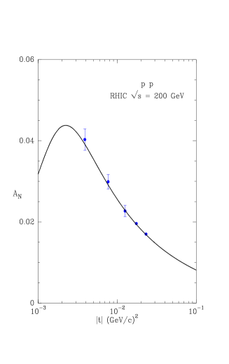
Figure 2: (Left): $\rho$ for $pp$ ($\bar{p}p$) elastic scattering as a function of $\sqrt{s}$ (Taken from Ref. (4)). (Right): The analyzing power $A_{N}$ versus $t$ at RHIC energy. The prediction is taken from Ref. (8) and the data from Ref. (9).

Why should $\rho$ be measured at the LHC [7] ?

• Real and imaginary parts of the scattering amplitude must obey dispersion relations according to local quantum field theory

• In string theory extra dimensions could generate observable non-local effects and therefore a violation of dispersion relations

• We can make a simple model to break polynomial boundness in some regions of the analyticity domain, leading for example to $\rho=0.21$ at 14TeV

• According to the BSW model, which satisfies dispersion relations, one should find instead $\rho=0.122\pm 0.003$

• Dispersion relations could be also violated if $\sigma_{tot}$ beyond the LHC energy, behaves very differently, due to some new physics.

• The highest energy where one has a reliable value of $\rho$ is at $\sqrt{s}=546\mbox{GeV}$, $\rho=0.135\pm 0.007$, since the Tevatron value $\rho=0.140\pm 0.069$ is useless

For all these reasons one needs an accurate value of $\rho$ at LHC.
Before moving to the non-forward region it is worth mentioning another test of the BSW amplitude, by means of the analyzing power $A_{N}$, near the very forward direction. In this kinematic region, the so called Coulomb nuclear interference (CNI) region, $A_{N}$ results from the interference of the Coulomb amplitude which is purely real, with the imaginary part of the hadronic non-flip amplitude, namely $a(s,t)$, if one assumes that there is no contribution from the single-flip hadronic amplitude [8]. This is what we have done in the calculation of the curve displayed in Fig. 2 (Right) compared to some new data from STAR which confirms the absence of single-flip hadronic amplitude and the right determination of $\mbox{Im}~{}a(s,t)$ in the CNI region [9].

3.2 Non-forward region

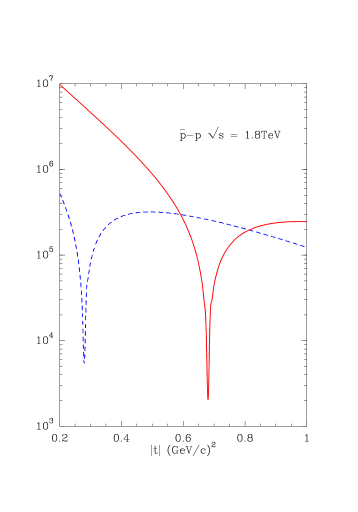
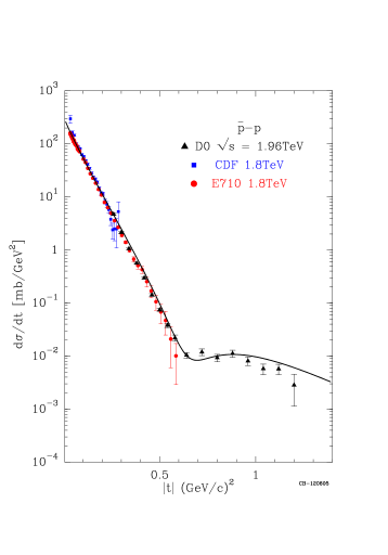
Figure 3: (Left): The absolute value of the $\bar{p}p$ elastic scattering amplitude, solid curve $|\mbox{Im}~{}a(s,t)|$, dashed curve $|\mbox{Re}~{}a(s,t)|,$ versus $t$ at $\sqrt{s}=1.8\mbox{TeV}$. (Right): The corresponding $d\sigma/dt$, prediction from Ref. (10), new D0 data from Ref. (11).

This kinematic region allows us to understand the behavior of the differential cross section from the $t$-dependence of the real and imaginary parts of the scattering amplitude, which have both some zeros at different $t$ values, as shown in Figs. 3 and 4 (Left). The imaginary part dominates over the real part, except when the imaginary part has a zero, producing either a shallow dip (or shoulder) for ${\bar{p}p}$ at $\sqrt{s}=1.8\mbox{GeV}$, as in Fig. 3 (Right) around $|t|=0.6\mbox{GeV}^{2}$, or a real dip for $pp$ at $\sqrt{s}=7\mbox{GeV}$, as in Fig. 4 (Right) around $|t|=0.5\mbox{GeV}^{2}$. Our prediction is in excellent agreement with the Tevatron data and although we predict the right position of the dip at LHC, we seem to underestimate the forward slope and to overestimate the cross section in the region of the second maximum, determined by TOTEM [5].

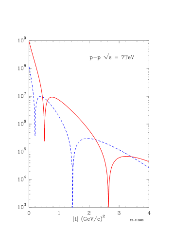
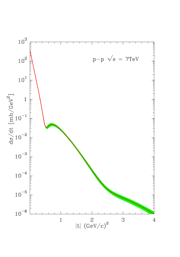
Figure 4: (Left): The absolute value of the $pp$ elastic scattering amplitude, solid curve $|\mbox{Im}~{}a(s,t)|$, dashed curve $|\mbox{Re}~{}a(s,t)|,$ versus $t$ at $\sqrt{s}=7\mbox{TeV}$. (Right): The corresponding differential cross section (Taken from Ref.(12)).

4 Concluding remarks

LHC is opening up a new area for $pp$ elastic scattering and TOTEM has confirmed the following basic features expected at LHC from BSW: $\sigma_{tot}$ and $\sigma_{el}/\sigma_{tot}$ increase, the diffraction peak is still shrinking, the dip position is moving in and the second maximum is moving up. So far one observes only partial quantitative agreement with the BSW approach, but more data are needed, in particular from ATLAS-ALFA. One should not forget the relevance of the measurement of $\rho$.

References

- [1] C. Bourrely, J. Soffer and T.T. Wu, Phys. Rev. D 19, 3249 (1979).
- [2] C. Bourrely, J. Soffer and T.T. Wu, Nucl. Phys. B 247, 15 (1984).
- [3] C. Bourrely, J. Soffer and T.T. Wu, Z. Phys. C 37, 369 (1988); Erratum-ibid 53, 538 (1992).
- [4] C. Bourrely, J. Soffer and T.T. Wu, Eur. Phys. J. C 28, 97 (2003).
- [5] For new LHC data see M. Deile, these proceedings.
- [6] H. Cheng and T.T. Wu, Phys. Rev. Lett. 24, 1456 (1970) (See also H. Cheng and T.T. Wu, Expanding Protons: Scattering at High Energies (MIT Press, Cambridge, MA, 1987)).
- [7] C. Bourrely, N.N. Khuri, A. Martin, J. Soffer and T.T. Wu, Invited talk at the ” XIth International Conference on Elastic and Diffractive Scattering: Towards High Energy Frontiers”, Château de Blois, (France), 15-20/05/2005, M. Haguenauer, B. Nicolescu and J. Tran Thanh Van (Eds.) The Gioi Publishers, Vietnam, pp. 41-44 (2006).
- [8] C. Bourrely, J. Soffer and T.T. Wu, Phys. Rev. D 76, 053002 (2007).
- [9] For new STAR data see D. Svirida, these proceedings and L. Adamczyk et al., arXiv:1206.1928v1 [nucl-ex].
- [10] C. Bourrely, J. Soffer and T.T. Wu, Eur. Phys. J. C 71, 1601 (2011).
- [11] V.M. Abazov et al., arXiv:1206.0687v1 [hep-ex].
- [12] C. Bourrely, J. Myers, J. Soffer and T.T. Wu, Phys. Rev. D 85, 096009 (2012).