On Dynamical Justification of Quantum

Scattering Cross Section

Alexander Komech

Fakultät für Mathematik, Universität Wien
and Institute for Information Transmission Problems RAS
e-mail: alexander.komech@univie.ac.at

A dynamical justification of quantum differential cross section in the context of long time transition to stationary regime for the Schrödinger equation is suggested. The problem has been stated by Reed and Simon.

Our approach is based on spherical incident waves produced by a harmonic source and the long-range asymptotics for the corresponding spherical limiting amplitudes. The main results are as follows: i) the convergence of spherical limiting amplitudes to the limit as the source increases to infinity, and ii) the universally recognized formula for the differential cross section corresponding to the limiting flux.

The main technical ingredients are the Agmon–Jensen–Kato’s analytical theory of the Green function, Ikebe’s uniqueness theorem for the Lippmann–Schwinger equation, and some adjustments of classical asymptotics for the Coulomb potentials.

Keywords: Schrödinger equation, Coulomb potential, spherical waves, plane waves, scattering, scattering operator, differential cross section, limiting amplitude, spherical limiting amplitude, Lippmann–Schwinger equation, oscillatory integrals.

MSC classification: 81U, 35P25,47A40

1 Introduction

The differential cross section is the main observable in quantum scattering experiments. This concept was first introduced to describe the Rayleigh scattering of sunlight and the Rutherford alpha-particle scattering as the quotient

$$\sigma(\theta)={j_{a}^{\rm sc}(\theta)}/|{j^{\rm in}}|.$$ (1.1)

Here, $j^{\rm in}$ is the incident stationary flux, and $j_{a}^{\rm sc}(\theta)$ is the angular density of the scattered stationary flux $j^{\rm sc}(x)$ in the direction $\theta\in\mathbb{R}^{3}$, $|\theta|=1$ (see Fig. 1):

$${j_{a}^{\rm sc}(\theta)}=\lim_{R\to\infty}R^{2}j^{\rm sc}(R\theta)\cdot\theta.$$ (1.2)

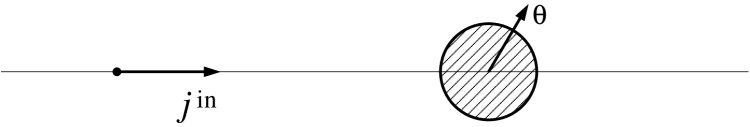
Figure 1: Incident flux and scatterer.

In both scattering processes studied by Rayleigh and Rutherford the concept of differential cross section is well-established in the framework of the corresponding dynamical equations: the Maxwell equations in the case of Rayleigh scattering and the Newton equations in the case of Rutherford scattering.

On the other hand, a satisfactory dynamical justification of quantum scattering cross section is still missing in the framework of the Schrödinger equation

$$i\dot{\psi}(x,t)=H\psi(x,t):=-\frac{1}{2}\Delta\psi(x,t)+V(x)\psi(x,t),\qquad x\in\mathbb{R}^{3}.$$ (1.3)

The problem has been stated and discussed by Reed and Simon in [22], pp. 355–357. We suggest the solution for the first time, as far as we are aware. The corresponding charge and flux densities are defined as

$$\rho(x,t)=|\psi(x,t)|^{2},\qquad j(x,t)={\rm Im{\hskip 1.42262pt}}[\overline{\psi(x,t)}\nabla\psi(x,t)].$$ (1.4)

These densities satisfy the charge continuity equation

$$\dot{\rho}(x,t)+{\rm div~{}}j(x,t)=0,\qquad(x,t)\in\mathbb{R}^{4}.$$ (1.5)

We justify the formula for the differential cross section

$$\sigma(k,\theta)=16\pi^{4}|T(|k|\theta,k)|^{2},$$ (1.6)

which is universally recognized in physical and mathematical literature (see, for example, [13, 20, 22, 25, 28]). We denote by $k\in\mathbb{R}^{3}$ the ‘wave vector’ of the incident plane wave

$$\psi^{\rm in}(x,t)=e^{i(kx-E_{k}t)},\qquad E_{k}:=\frac{1}{2}k^{2}.$$ (1.7)

Let the brackets $(\cdot,\cdot)$ denote the Hermitian scalar product in the complex Hilbert space ${\cal L}^{2}:=L^{2}(\mathbb{R}^{3})$, as well as its extension to the duality between the weighted Agmon–Sobolev spaces, see (2.2) and (7.11). The $T$-matrix is given by

$$T(k^{\prime},k):=\frac{1}{(2\pi)^{3}}(T(E_{k}+i0)e^{ikx},e^{ik^{\prime}x}),\qquad k^{\prime},k\in\mathbb{R}^{3},$$ (1.8)

which is the integral kernel of the operator $T(E_{k}+i0):=V-VR(E_{k}+i0)V$ (see Section 25 of [17]) in the Fourier transform

$$\hat{\psi}(k)=\int e^{-ikx}\psi(x)dx,\qquad\psi\in C_{0}^{\infty}(\mathbb{R}^{3}).$$ (1.9)

Here, $R(E):=(H-E)^{-1}$ is the resolvent of the Schrödinger operator $H$.

It is well known that the integral kernel $S(k^{\prime},k)$ of the scattering operator $S$ in the Fourier transform reads as

$$S(k^{\prime},k)=\delta(k^{\prime}-k)-i\pi\delta(E_{k^{\prime}}-E_{k})T(k^{\prime},k),~{}~{}~{}k^{\prime},k\in\mathbb{R}^{3}$$ (1.10)

(see [3, 20, 22, 25]). The commonly used ‘naive scattering theory’ consists of the following statements [22, 24, 25].
I. The incident wave is identified with the plane wave (1.7), which propagates in the direction of the wave vector $k$ and is a solution to the free Schrödinger equation (1.3) with $V(x)=0$.

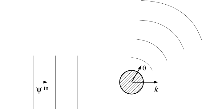
Figure 2: Incident plane wave and outgoing spherical wave.

II. The corresponding ‘scattered’ solution to (1.3) is identified by its long time asymptotics on any bounded region $|x|<R$,

$$\psi(x,t)\sim A(x)e^{-iE_{k}t},\qquad t\to\infty,$$ (1.11)

where the amplitude $A(x)$ is expressed by

$$A(x)=e^{ikx}-R(E_{k}+i0)[V(x)e^{ikx}].$$ (1.12)

This amplitude admits the following ‘spherical’ long range asymptotics (3.58) of [3, Ch. 4]

$$A(x)\sim e^{ikx}+a(k,\theta)\frac{e^{i|k|\cdot|x|}}{|x|},\qquad x|\to\infty,\qquad\theta:=x/|x|~{};$$ (1.13)

see Fig. 2.
III. By (1.4), asymptotics (1.13) give

$$j^{\rm in}=k,\qquad j_{a}^{\rm sc}(\theta)=|a(k,\theta)|^{2}|k|,$$ (1.14)

and hence the differential cross section reads

$$\sigma(k,\theta)=|a(k,\theta)|^{2}.$$ (1.15)

It is well known that $a(k,\theta)$ is proportional to the $T$-matrix (formula (97a) of [22]):

$$a(k,\theta)=-4\pi^{2}T(|k|\theta,k).$$ (1.16)

Hence, (1.15) reads as (1.6).

A heuristic derivation of relations (1.11), (1.12) can be found in [22], pp. 355–357. However, a mathematically consistent justification of the relations in a time dependent picture was not suggested until now. Moreover, relation (1.6) was considered up to now as the definition of the differential cross section: see formulas (1.2) and (A.1.6) of [13], formula (96) of [22], and Definition 7.9 on p. 254 of [29].

The main problem in mathematical justification of (1.11) and (1.12) is related to the lack of a consistent model for the incident wave $\psi^{\rm in}(x,t)$, securing convergence (1.11) to a stationary regime, and at the same time satisfies the ‘adiabatic condition’

$$\psi^{\rm in}(x,t)\to 0,\qquad t\to-\infty,\quad x\in\mathbb{R}^{3},$$ (1.17)

which is in the spirit of the scattering theory. The plane incident wave (1.7) in the ‘naive scattering theory’ does not satisfy (1.17), since the wave occupies the entire space. The plane wave is a solution to the free Schrödinger equation

$$i\dot{\psi}(x,t)=-\frac{1}{2}\Delta\psi(x,t),\qquad x\in\mathbb{R}^{3}.$$ (1.18)

The adiabatic condition (1.17) in acoustic scattering is provided by the ‘semi-infinite’ incident plane wave

$$\psi^{\rm in}(x,t)=\Theta(|k|t-kx)e^{i(kx-|k|t)}$$

for $t<0$, where $\Theta$ is the Heaviside function. This incident wave is a solution to the acoustic equation

$$\ddot{\psi}(x,t)=\Delta\psi(x,t),\qquad|x|>R,$$ (1.19)

for $t<-R$ if the scatterer is located in the region $|x|\leq R$. The similar incident plane wave can be constructed for the Maxwell equations, which makes apparent the meaning of the differential cross section in the Rayleigh scattering.

On the other hand, a similar semi-infinite incident plane wave does not exist in the case of the Schrödinger equation. Indeed, we may fix $R\gg|k|D$ and take the semi-infinite plane wave

$$\psi^{\rm in}(x)=\Theta(-R-kx)e^{ikx}$$

as the initial condition at $t=0$. However, the corresponding solution does not satisfy the adiabatic condition for $t\to-\infty$. The problem is of great importance also in the context of the quantum field theory, where the incident and outgoing plane waves play the fundamental role [20, 23, 24, 28].

In the traditional approach, the incident wave is a specific initial field, which is a solution to the corresponding free wave equation in the entire space. On the other hand, in practice, the incident wave is a beam of particles or light produced by a macroscopic source and satisfies the free wave equation only outside the source. One could expect that, for a large time, the incident wave near the scatterer will asymptotically be a free plane wave if the source is ‘monochromatic’ and its distance from the scatterer, $D$, tends to infinity. This model obviously corresponds to spherical incident waves, which are standard devices in optical and acoustic scattering [4].

We justify formula (1.6) in the following steps:
A. First, we prove the limiting amplitude principle for the Schrödinger equation (1.3) with harmonic source; i.e., the long time convergence to a stationary harmonic regime with a ‘spherical limiting amplitude’, which does not depend on initial state.
B. Second, we prove the convergence of the spherical limiting amplitudes to the plane limiting amplitude when the source goes off to infinity: $D\to\infty$.
C. We deduce from A and B that relations (1.11)–(1.13) and (1.15) hold true in this double limit: first, as $t\to\infty$, and then, as $D\to\infty$.
D. Finally, we establish the second relation of (1.14) for the scattered flux

$$j^{\rm sc}(x,t):=j_{\infty}(x,t)-j^{\rm in},$$ (1.20)

where $j_{\infty}(x,t)$ is the double limit of the current (1.4), and $j^{\rm in}:=\lim_{|x|\to\infty}j_{\infty}(x,t)$. Now formula (1.6) follows from (1.15) and (1.16).

Our technical novelties are as follows. We prove the limiting amplitude principle A, developing the Agmon–Jensen–Kato’s theory of the resolvent of the Schrödinger operator [1, 16, 17]. The proof of the convergence B relies on a novel application of Ikebe’s uniqueness theorem for the Lippmann–Schwinger equation [3, 14] and on uniform bounds for the Coulomb potentials (4.6), (4.14), (4.25). These bounds are due to novel asymptotics for the Coulomb potentials (4.4), which are regularized at the zero point (the corresponding bound (3.51) of [3, Ch. 4], is correct only for $|x|\geq\delta>0$ due to the singularity of the main term in the asymptotics (3.50) of [3, Ch. 4]). Moreover, we adjust the estimates for the remainders in the long range asymptotics of the Coulomb potentials, which dates back to Povzner and Ikebe [14, 21] (see (7.4) and (7.9)).

Note that formula (1.4) describes the wave flux corresponding to the one-particle Schrödinger equation (1.3). Respectively, the many-particle interpretation of the cross section (1.1) is not straightforward. However, it is worth noting that definition (1.20) means the principle of superposition for the currents corresponding to the many-particle scattering. Thus, the validity of the second relation of (1.14), as proved in our final Theorem 8.2, suggests the many-particle interpretation.

We note that Theorem 8.2 was not established in Chapter 9 of [17], which is the previous version of present paper. Our progress relies on the novel estimates (7.4) and (7.9). Moreover, here we consider general case of the Schrödinger operator $H$ with nonempty discrete spectrum, in contrast to [17], Ch. 9. Finally, here we adjust our basic assumptions and proofs.

We make some comments on the known arguments for formula (1.6). The traditional physical approach [25] is based on random incident wave packets $\psi^{\rm in}(x,0)$, which are asymptotically proportional to the plane waves $e^{ikx}$:

$$|\hat{\psi}^{\rm in}(k^{\prime},0)|^{2}\to\delta(k^{\prime}-k).$$ (1.21)

The known mathematical justifications reside in Dollard’s fundamental result [7] on scattering into cones. This result is used in [27] for a clarifying treatment of formula (1.6). Namely, the normalized angular distribution of a finite charge, scattered for infinite time, converges to the normalized function (1.6) in the limit (1.21).

Dollard’s result was refined in [6, 15] and in Section 3-3 of [2], where the flux across the surface theorem is proved. This result was later developed in [8, 9, 11, 26] and applied for justification of formula (1.6) in the context of the Bohmian particle mechanics and incident stationary random processes constructed of normalized wave packets (1.6) in the limit (1.21). For a survey, see [10]. It is worth noting that we do not exclude the discrete spectrum of the Schrödinger operator $H$, in contrast to [8].

We point out that all the previous results give the same expression (1.6) for the differential cross section, though these results were not concerned with the long time transition to a stationary regime.

Our paper is organized as follows. The main results are stated in Section 2. The limiting amplitude principle is established in Section 3. In Section 4 we obtain long range asymptotics and uniform bounds for the spherical limiting amplitudes. Next, in Sections 5 and 6 we prove convergence B and the corresponding convergence for the flux. Finally, in Sections 7 and 8 we verify formulas (1.16) and (1.14), which justify (1.15) and (1.6).

Acknowledgments. The author thanks E. Kopylova and H. Spohn for useful discussions and remarks.

2 Main results

We consider the Schrödinger equation with harmonic source:

$$\left\{\begin{array}[]{l}i\dot{\psi}(x,t)=H\psi(x,t)+\rho_{q}(x){\hskip 1.42262pt}e^{-iE_{k}t},\qquad t>0\vskip 6.0pt plus 2.0pt minus 2.0pt\\ \psi(x,0)=\psi^{0}(x)\end{array}\right|\qquad x\in\mathbb{R}^{3}.$$ (2.1)

Here, $H=-\frac{1}{2}\Delta+V(x)$, $E_{k}=k^{2}/2$ for $k\in\mathbb{R}^{3}\setminus 0$, and $\rho_{q}(x):=|q|\rho(x-q)$ is the form factor of the source.

We mean that our model suits the physics of quantum scattering. Namely, the incident wave is produced by time periodic source, like a heated cathode in an electron gun. The source is not at infinity, though its distance from the scatterer is sufficiently large.

The solution $\psi(x,t)$ describes the spherical waves produced by the source. The spherical waves look like plane waves near the scatterer in the limit $|q|\to\infty$. The source is described by a density factor $\rho_{q}(x)$, where the factor $|q|$ is introduced for a suitable normalization, see (2.14) below.

The weighted Agmon–Sobolev spaces ${\cal H}^{s}_{\sigma}={\cal H}^{s}_{\sigma}(\mathbb{R}^{3})$, $s,\sigma\in\mathbb{R}$, are defined as follows. Let ${\cal L}^{2}_{\sigma}={\cal L}^{2}_{\sigma}(\mathbb{R}^{3})$ be the Hilbert space of measurable functions in $\mathbb{R}^{3}$ with norm

$$\|\psi\|_{{\cal L}^{2}_{\sigma}}^{2}=\int\langle x\rangle^{2\sigma}|\psi(x)|^{2}dx,\qquad\langle x\rangle:=\sqrt{x^{2}+1}.$$ (2.2)

Definition 2.1.

${\cal H}^{s}_{\sigma}={\cal H}^{s}_{\sigma}(\mathbb{R}^{3})$ denotes the Hilbert space of tempered distributions $\psi(x)$ with finite norm

$$\|\psi\|_{{\cal H}^{s}_{\sigma}}:=\|\langle\nabla\rangle^{s}\psi\|_{{\cal L}^{2}_{\sigma}}<\infty.$$ (2.3)

We will assume the following conditions.
H0. The initial state $\psi^{0}$ is a function from the space ${\cal H}^{2}_{\sigma_{0}}$ with some $\sigma_{0}>5/2$.
H1. For some $\varepsilon_{1}>0$,

$$\sup\limits_{x\in\mathbb{R}^{3}}\langle x\rangle^{4+\varepsilon_{1}}|\partial^{\alpha}\rho(x)|<\infty,\qquad|\alpha|\leq 2.$$ (2.4)

H2. The following Wiener condition holds:

$$\hat{\rho}(|k|\theta):=\int e^{i|k|\theta x}\rho(x)dx\neq 0,\qquad\theta\in\mathbb{R}^{3},\ \ |\theta|=1.$$ (2.5)

H3. The potential $V(x)$ is a real $C^{2}$-function satisfying the condition

$$\sup\limits_{x\in\mathbb{R}^{3}}\langle x\rangle^{5+\varepsilon_{2}}|\partial^{\alpha}V(x)|<\infty,\qquad|\alpha|\leq 2,$$ (2.6)

with some $\varepsilon_{2}>0$.

Finally, we introduce our key spectral assumption. Denote

$${\cal M}_{\sigma}:=\{\psi\in{\cal L}^{2}_{-\sigma}:\psi+R_{0}(0)V\psi=0\},$$

where $R_{0}(E):=(-\frac{1}{2}\Delta-E)^{-1}$ is the free resolvent. The space ${\cal M}_{\sigma}={\cal M}$ does not depend on $\sigma\in(1/2,(5+\varepsilon_{2})/2)$ by the arguments preceding Lemma 3.1 of [16].
H4. We assume:

$${\bf The\ Spectral\ Condition:}~{}~{}~{}~{}~{}~{}~{}~{}~{}~{}~{}~{}~{}~{}~{}~{}~{}~{}~{}{\cal M}=0.~{}~{}~{}~{}~{}~{}~{}~{}~{}~{}~{}~{}~{}~{}~{}~{}~{}~{}~{}~{}~{}~{}~{}~{}~{}~{}~{}~{}$$ (2.7)

This condition holds for generic potentials, see the discussion preceding Lemma 3.1 in [16].

Let us outline our plan.
I. First, we will prove the limiting amplitude principle:

$$~{}~{}\psi(x,t)\sim\varphi_{q}(x,t)=B_{q}(x)e^{-iE_{k}t}+\sum_{1}^{N}C^{l}_{q}\psi_{l}(x)e^{-iE^{l}t},~{}~{}~{}t\to\infty,$$ (2.8)

where $\psi_{l}(x)$ are the eigenfunctions of $H$ corresponding to the eigenvalues $E^{l}<0$. The asymptotics hold in ${\cal H}^{2}_{-\sigma}$ with any $\sigma>5/2$, and the limiting amplitude $B_{q}(x)$ is given by

$$B_{q}(x)=R(E_{k}+i0)\rho_{q}.$$ (2.9)

The coefficients $C^{l}$ depend on the initial state $\psi(x,0)$. On the other hand, it is crucially important that the coefficients $C^{l}$ converge as $|q|\to\infty$, while the eigenfunctions $\psi_{l}(x)$ decay rapidly at infinity by Agmon’s theorem [1], Theorem 3.3 (see also Theorem 20.7 of [17]). Hence, the sum over the discrete spectrum on the right-hand side of (2.8) does not contribute to the scattering cross section, and we will omit it almost everywhere below.
II. Second, denoting $B_{D}(x):=B_{q_{D}}(x)$, where $q_{D}:=-nD$ with $n:=k/|k|$ and $D>0$, we establish the following ‘spherical version’ of long range asymptotics (1.13):

$$~{}~{}~{}~{}~{}~{}~{}B_{D}(x) \sim b_{D}(n)\Big{[}\frac{|q_{D}|}{|x-q_{D}|}e^{i|k|(|x-q_{D}|-|q_{D}|)}+a_{D}(k,\theta)\frac{e^{i|k|\cdot|x|}}{|x|}\Big{]}$$ (2.10)

$${\rm as}\quad|x-q_{D}|\to\infty,\quad|x|\to\infty,$$

where $\theta:=x/|x|$ and $b_{D}(n):=b(n)e^{i|k|D}$ with $b(n)\neq 0$; see Fig. 3. The asymptotics (2.10) mean that the difference between the left-hand side and the right-hand side converges to zero.

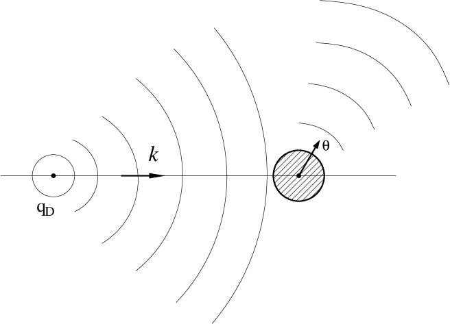
Figure 3: Incident and outgoing spherical waves.

III. Further, we prove the convergence of the spherical limiting amplitudes, which is our central result: for $k\neq 0$

$$A_{D}(x):=B_{D}(x)/b_{D}(n)\to A(x),\qquad D\to\infty,$$ (2.11)

where $A(x)$ is expressed by (1.12).
IV. At last, (2.11) implies the asymptotics of the corresponding limiting solutions $\varphi_{D}(x,t):=\varphi_{q_{D}}(x,t)$ (neglecting the last sum of (2.8))

$$~{}~{}\varphi_{D}(x,t)/b_{D}(n)\to A(x)e^{-iE_{k}t},\qquad D\to\infty,\quad(x,t)\in\mathbb{R}^{4},$$ (2.12)

and of the corresponding flux (1.4):

$$\!\!\!\!\!\!\!\!\!\!\!\!\!\!\!\!\!\!\!\!j_{D}(x)={\rm Im{\hskip 1.42262pt}}[\overline{\varphi_{D}(x,t)}\nabla\varphi_{D}(x,t)]\!\!\!\! \!\!\!\!\longrightarrow\!\!\!\! \!\!\!\!j_{\infty}(x)=|b(n)|^{2}{\rm Im{\hskip 1.42262pt}}[\overline{A(x)}\nabla A(x)],$$

$$\!\!\!\!D\to\infty\!\!\!\!$$

Here, we again neglect the last sum of (2.8), for it does not contribute to the currents at large $|x|$.
V. Finally, we calculate the long range asymptotics of $A(x)$ as $|x|\to\infty$ and show that the convergence (2) and formula (1.12) justify (1.1), (1.6) in the limit $D\to\infty$.

Let us comment on our methods. We derive the limiting amplitude principle (2.8) from the dispersion decay in weighted energy norms by a suitable development of Agmon–Jensen–Kato’s methods [1, 16, 17]. The long range asymptotics (2.10) is deduced from the ‘spherical version’ (4.1) of the Lippmann–Schwinger equation and a refinement of Lemma 3.2 from [3, Ch. 4]. One of our key observations is that the spherical incident wave from (2.10) becomes asymptotically the plane incident wave from (1.13) as the source goes off to infinity:

$$\frac{|q_{D}|}{|x-q_{D}|}e^{i|k|(|x-q_{D}|-|q_{D}|)}\to e^{ikx},\qquad D\to\infty.$$ (2.14)

In this limit, the picture of Fig. 3 becomes the one of Fig. 2. We derive convergence (2.11) from asymptotics (2.10) by the Sobolev embedding theorem and the Ikebe uniqueness theorem for the Lippmann–Schwinger equation [14] (Theorem 3.1 of [3, Ch. 4]). Finally, we prove the second formula of (1.14) for the flux (1.20) in Theorem 8.2. We deduce it from the decay of the oscillatory integrals (8.8), which is due to the interference of the incident and scattered waves.

3 Limiting amplitude principle

We deduce the limiting amplitude principle (2.8) from the dispersion decay in weighted energy norms [16, 17].

Lemma 3.1.

Assume that conditions H0–H4 hold and $k\in\mathbb{R}^{3}$. Then
i) The limiting amplitude principle (2.8) holds in the norm of ${\cal H}^{2}_{-\sigma}$ with any $\sigma>5/2$.
ii) $C^{l}_{q}$ converge to the limit $C^{l}$ as $|q|\to\infty$, and the limiting amplitude is given by (2.9).

Proof.

We should prove that

$$\psi(x,t)=B_{q}(x)e^{-iE_{k}t}+\sum_{1}^{N}C^{l}_{q}\psi_{l}(x)e^{-iE^{l}t}+r(x,t),$$ (3.1)

where

$$C^{l}_{q}\to C_{l},\qquad|q|\to\infty;\qquad\|r(\cdot,t)\|_{{\cal H}^{2}_{-\sigma}}\to 0,\qquad t\to\infty.$$ (3.2)

The solution to the Cauchy problem (2.1) is unique and is given by the Duhamel representation

$$\psi(t)=U(t)\psi^{0}-i\displaystyle\int_{0}^{t}e^{-iE_{k}s}U(t-s)\rho_{q}~{}ds.$$ (3.3)

Here, $U(t)$ is the dynamical group of equation (2.1) with $\rho_{q}=0$, and the first term in the right-hand side admits the expansion

$$U(t)\psi^{0}=\sum_{1}^{N}C^{l}\psi_{l}e^{-iE^{l}t}+r_{0}(t),$$ (3.4)

where $C^{l}$ are independent of $q$, and

$$\|r_{0}(t)\|_{{\cal H}^{2}_{-\sigma}}\leq C\langle t\rangle^{-3/2}.$$ (3.5)

This decay follows similarly to the dispersion decay in the norm ${\cal H}^{0}_{-\sigma}$, as established in (10.9) of [16], with suitable refinement of the resolvent high energy decay (see Theorem 17.1 of [17]). Here, the assumptions H0 and H3–H4 are essential.
On the other hand, the second term on the right-hand side of (3.3) can be written as

$$I(t)=-i\displaystyle\int_{0}^{t}e^{-iE_{k}s}U(t-s)\rho_{q}~{}ds=-ie^{-iE_{k}t}\int_{0}^{t}e^{iE_{k}\tau}U(\tau)\rho_{q}d\tau.$$ (3.6)

Here, $\rho_{q}\in{\cal H}^{2}_{\sigma_{1}}$ with some $\sigma_{1}>5/2$ by H1. Hence, similarly to (3.4) and (3.5),

$$U(\tau)\rho_{q}=\sum_{1}^{N}D^{l}_{q}\psi_{l}e^{-iE^{l}\tau}+r_{q}(\tau),$$ (3.7)

where

$$\|r_{q}(\tau)\|_{{\cal H}^{2}_{-\sigma}}\leq C_{q}\langle\tau\rangle^{-3/2}.$$ (3.8)

Finally, the eigenfunctions $\psi_{l}(x)\in{\cal L}^{2}_{s}$ with any $s\in\mathbb{R}$ by Agmon’s theorem [1, Theorem 3.3], (see also Theorem 20.7 of [17]). Hence, (2.4) implies that

$$D^{l}_{q}=\langle\rho_{q},\psi_{l}\rangle=|q|\int\rho(x-q)\psi_{l}(x)dx={\cal O}(|q|^{-3-\varepsilon_{1}}),\qquad|q|\to\infty.$$ (3.9)

Therefore, $C^{l}_{q}=C^{l}+D^{l}_{q}\to C^{l}$ as $|q|\to\infty$, and

$$I(t)\sim B_{q}(x)e^{-iE_{k}t}+{\cal O}(|q|^{-3-\varepsilon_{1}}),\qquad t\to\infty.$$ (3.10)

Here, the asymptotics hold in ${\cal H}^{2}_{-\sigma}$, and the limiting amplitude is given by

$$B_{q}(x)=-i\int_{0}^{\infty}e^{iE_{k}\tau}U(\tau)\rho_{q}d\tau=-i\int_{0}^{\infty}e^{i(E_{k}+i0)\tau}U(\tau)\rho_{q}d\tau,$$ (3.11)

which can be written as (2.9). This proves (3.1). ∎

4 Spherical waves

In this section we obtain long range asymptotics (2.10). Denote $R=R(E_{k}+i0)$ and $R_{0}=R_{0}(E_{k}+i0)$, where $R_{0}(E)=(H_{0}-E)^{-1}$ is the resolvent of the free Schrödinger operator $H_{0}=-\displaystyle\frac{1}{2}\Delta$. Rewriting formula (2.9) for the limiting amplitude as the following ‘spherical version’ of the Lippmann–Schwinger equation, this gives

$$B_{q}(x)=R_{0}\rho_{q}(x)-R_{0}VB_{q}(x),$$ (4.1)

since $R=R_{0}-R_{0}VR$. The free Schrödinger resolvent $R_{0}(E)$ is the integral operator with kernel

$$R_{0}(E,x,y)=\frac{e^{i\sqrt{2E}|x-y|}}{2\pi|x-y|},\qquad E\in\mathbb{C}\setminus[0,\infty).$$

Therefore, $R_{0}$ is the integral operator with kernel

$$R_{0}(E_{k}+i0,x,y)=\frac{e^{i|k||x-y|}}{2\pi|x-y|},$$ (4.2)

because $\sqrt{2(E_{k}+i0)}=|k|$.

For the first term on the right-hand side of (4.1), asymptotics (2.10) follow by a suitable modification of Lemma 3.2 from [3, Ch. 4]. Let

$$S=\{\theta\in\mathbb{R}^{3}:|\theta|=1\}$$ (4.3)

be the unit sphere.

Lemma 4.1.

Under condition H1 with $\alpha=0$,

$$R_{0}\rho_{q}(x)=b\Big{(}\frac{x-q}{|x-q|}\Big{)}\frac{|q|}{1+|x-q|}e^{i|k||x-q|}+K(x-q),\qquad x\in\mathbb{R}^{3}.$$ (4.4)

Here, the amplitude $b\in C^{1}(S)$, and

$$b(\theta)=\frac{1}{2\pi}{\hat{\rho}(|k|\theta)},\qquad|\theta|=1,$$ (4.5)

where $\hat{\rho}(k)$ denotes the Fourier transform (1.9). The remainder admits the bound

$$|K(x-q)|\leq C|q|(1+|x-q|)^{-1-\varepsilon_{1}},\qquad x\in\mathbb{R}^{3}.$$ (4.6)

Proof.

This lemma follows by the arguments from the proof of Lemma 3.2 from [3, Ch. 4], with $|x|$ substituted almost everywhere by $|x|+1$. Moreover, H1 with $\alpha=0$ implies that $\hat{\rho}\in C^{1}_{b}(\mathbb{R}^{3})$. Hence, $b\in C^{1}(S)$ by (4.5). ∎

As a corollary, we obtain the bound

$$|R_{0}\rho_{q}(x)|\leq\frac{C|q|}{1+|x-q|},\qquad x\in\mathbb{R}^{3}.$$ (4.7)

Remark 4.2.

Our asymptotics (4.4) and the estimate (4.6) differ from similar ones (3.50) and (3.51) of [3, Ch. 4], which hold only for $|x|\geq\delta>0$.

For the second term on the right-hand side of (4.1) we need two additional technical lemmas.

Lemma 4.3.

Under conditions H1 and H3 the following bound holds for $k\neq 0$:

$$\sup_{q\in\mathbb{R}^{3}}\|VB_{q}(x)\|_{{\cal L}^{2}_{\sigma}}<\infty\quad\mbox{for any}\quad\sigma<5/2+\varepsilon_{2}.$$ (4.8)

Proof.

The Lippmann–Schwinger equation (4.1) implies

$$(1+VR_{0})VB_{q}=-VR_{0}\rho_{q}.$$ (4.9)

On the other hand, $(1+VR_{0})^{-1}=1-VR$. Hence,

$$VB_{q}=-(1-VR)VR_{0}\rho_{q}=-VR_{0}\rho_{q}+VRVR_{0}\rho_{q}.$$ (4.10)

Let us estimate each term on the right-hand side separately.
i) Condition (2.6) with $\alpha=0$ and bound (4.7) imply

$$|VR_{0}\rho_{q}(x)|\leq\frac{C|q|}{(1+|x-q|)(1+|x|)^{5+\varepsilon_{2}}},\quad x\in\mathbb{R}^{3}.$$ (4.11)

Therefore,

$$|VR_{0}\rho_{q}(x)|\leq\frac{C}{(1+|x|)^{4+\varepsilon_{2}}},\quad x\in\mathbb{R}^{3}.$$ (4.12)

Hence,

$$VR_{0}\rho_{q}\in{\cal L}^{2}_{\sigma},\qquad\sigma<5/2+\varepsilon_{2}.$$ (4.13)

Thus, the bound (4.8) holds for the first term on the right-hand side of (4.10).
ii) It remains to estimate the last term of (4.10). By (4.13) we have $RVR_{0}\rho_{q}\in{\cal L}^{2}_{-s}$ for any $s>1/2$, since the resolvent $R=R(E_{k}+i0):{\cal L}^{2}_{s}\to{\cal L}^{2}_{-s}$ is continuous by [16], Theorem 9.2, because $E_{k}>0$ for $k\neq 0$. Therefore, $VRVR_{0}\rho_{q}\in{\cal L}^{2}_{\sigma}$ for $\sigma<4.5+\varepsilon_{2}$ by (2.6) with $\alpha=0$. ∎

Lemma 4.4.

Under conditions H1 and H3 the following uniform decay holds:

$$\sup_{q\in\mathbb{R}^{3}}|R_{0}VB_{q}(x)|\leq C(1+|x|)^{-2},\quad x\in\mathbb{R}^{3}.$$ (4.14)

Proof.

By (4.2),

$$\begin{gathered}|R_{0}VB_{q}(x)|\leq C\int\frac{|VB_{q}(y)|}{|x-y|}dy=C\int_{0}^{\infty}\Big{[}\int\frac{|VB_{q}(r,\varphi,\theta)|d\varphi\sin\theta d\theta}{\sqrt{|x|^{2}+r^{2}-2|x|r\cos\theta}}\Big{]}r^{2}dr.\end{gathered}$$ (4.15)

Applying the Cauchy–Schwarz inequality to the inner integral,

$$|R_{0}VB_{q}(x)|\leq C\int_{0}^{\infty}\Big{[}\int|VB_{q}(r,\varphi,\theta)|^{2}d\varphi\sin\theta d\theta\Big{]}^{\frac{1}{2}}\Big{[}\int\frac{d\varphi\sin\theta d\theta}{|x|^{2}+r^{2}-2|x|r\cos\theta}\Big{]}^{\frac{1}{2}}r^{2}dr\\ =C\int_{0}^{\infty}\Big{[}\int|VB_{q}(r,\varphi,\theta)|^{2}d\varphi\sin\theta d\theta\Big{]}^{\frac{1}{2}}\Big{[}\frac{1}{|x|r}\log\frac{|x|+r}{||x|-r|}\Big{]}^{\frac{1}{2}}r^{2}dr.$$ (4.16)

Applying the same inequality to the last integral, this gives

$$|R_{0}VB_{q}(x)|$$

$$\leq C\Big{[}\int(1+r)^{2\sigma}|VB_{q}(r,\varphi,\theta)|^{2}d\varphi\sin\theta d\theta r^{2}dr\Big{]}^{\frac{1}{2}}\times\Big{[}\int_{0}^{\infty}\log\frac{|x|+r}{||x|-r|}~{}\frac{r^{2}dr}{|x|r(1+r)^{2\sigma}}\Big{]}^{\frac{1}{2}}$$

$$\leq C(\sigma)\Big{[}\int_{0}^{\infty}\log\frac{|x|+r}{||x|-r|}~{}\frac{rdr}{|x|(1+r)^{2\sigma}}\Big{]}^{\frac{1}{2}}=C(\sigma)\Big{[}\int_{0}^{\infty}\log\frac{1+s}{|1-s|}~{}\frac{|x|sds}{(1+s|x|)^{2\sigma}}\Big{]}^{\frac{1}{2}}$$ (4.17)

for $\sigma<5/2+\varepsilon_{2}$ by the uniform bound (4.8). Let us split the region of integration $(0,\infty)=(0,1/2)\cup(1/2,3/2)\cup(3/2,\infty)$ and observe that

$$\left.\begin{array}[]{ll}\log\frac{1+s}{|1-s|}={\cal O}(s),&\!\!\!\!\!\!\!\!\!\!\!\!\!s\in(0,1/2)\\ \vskip 3.0pt plus 1.0pt minus 1.0pt\cr\log\frac{1+s}{|1-s|}\in L^{1}(1/2,3/2)&\\ \vskip 3.0pt plus 1.0pt minus 1.0pt\cr\log\frac{1+s}{|1-s|}={\cal O}(s^{-1}),&\!\!\!\!\!\!\!\!\!\!\!\!s\in(3/2,\infty)\end{array}\right|$$ (4.18)

Then the integral (4.17) can be estimated as

$$C_{1}(\sigma)\Big{[}\int_{0}^{1/2}\frac{|x|s^{2}ds}{(1+s|x|)^{2\sigma}}+(1+|x|)^{1-2\sigma}+\int_{3/2}^{\infty}\frac{|x|ds}{(1+s|x|)^{2\sigma}}\Big{]}$$

$$=C_{1}(\sigma)\Big{[}|x|^{-2}\int_{0}^{|x|/2}\frac{r^{2}dr}{(1+r)^{2\sigma}}+(1+|x|)^{1-2\sigma}+\int_{3|x|/2}^{\infty}\frac{dr}{(1+r)^{2\sigma}}\Big{]}$$

$$\leq C_{2}(\sigma)(1+|x|)^{1-2\sigma}$$ (4.19)

for $2\sigma>1$. This gives (4.14), since we can take any $\sigma<5/2+\varepsilon_{2}$ by (4.8). ∎

Now we are ready to prove (2.10).

Proposition 4.5.

Asymptotics (2.10) hold under conditions H1–H3.

Proof.

The Lippmann–Schwinger equation (4.1) yields

$$VB_{q}(x)=-VR_{0}\rho_{q}(x)-VR_{0}VB_{q}(x).$$

Hence, (2.6) with $\alpha=0$ and (4.12), (4.14) imply that

$$|VB_{q}(x)|\leq\frac{C}{(1+|x|)^{4+\varepsilon_{2}}}.$$ (4.20)

Therefore, similarly to (4.4), we obtain the asymptotics

$$R_{0}VB_{q}(x)=c_{q}\Big{(}\frac{x}{|x|}\Big{)}\frac{e^{i|k||x|}}{1+|x|}+L_{q}(x),$$ (4.21)

where

$$|L_{q}(x)|\leq C(1+|x|)^{-1-\varepsilon_{2}}.$$ (4.22)

Now (4.1) and (4.4), (4.21) imply

$$B_{q}(x)\sim b\Big{(}\frac{x-q}{|x-q|}\Big{)}\frac{|q|}{|x-q|}e^{i|k||x-q|}+c_{q}\Big{(}\frac{x}{|x|}\Big{)}\frac{e^{i|k|\cdot|x|}}{|x|}$$ (4.23)

as $|x-q|\to\infty$ and $|x|\to\infty$. Denote $B_{D}(x):=B_{q_{D}}(x)$, where $q_{D}=-nD$ with $n=k/|k|$ and $D>0$. Then

$$B_{D}(x)\sim b(n)\Big{[}\frac{|q_{D}|}{|x-q_{D}|}e^{i|k||x-q_{D}|}+d_{D}(k,\theta)\frac{e^{i|k|\cdot|x|}}{|x|}\Big{]}$$ (4.24)

as $|x-q_{D}|\to\infty$ and $|x|\to\infty$, where $\theta:=x/|x|$, because $b(n)\sim\hat{\rho}(|k|n)\neq 0$ by (4.5) and the Wiener condition H2. This is the only point in our analysis, where the Wiener condition is called for. Finally, (4.24) can be written as (2.10) with $b_{D}(n):=b(n)e^{i|k|D}$ and $\displaystyle a_{D}(k,\theta)=d_{D}(k,\theta)e^{-i|k|D}$. ∎

The following corollary is of crucial importance in the next section.

Corollary 4.6.

Bound (4.7), asymptotics (4.21)–(4.22), and formula (4.1) imply

$$|B_{q}(x)|\leq\frac{C|q|}{1+|x-q|}+\frac{C}{(1+|x|)},\qquad x,q\in\mathbb{R}^{3}.$$ (4.25)

5 Plane wave limit

In this section we prove convergence (2.11) from the uniqueness of solution to the Lippmann–Schwinger equation

$$A(x)=e^{ikx}-R_{0}VA(x),$$ (5.1)

which is equivalent to (1.12) (see Lemma 7.1 below). First, we rewrite (4.1) with $q=q_{D}$ as

$$A_{D}(x)=R_{0}\rho_{q_{D}}(x)/b_{D}(n)-R_{0}VA_{D}(x),$$ (5.2)

where $A_{D}(x):=B_{D}(x)/b_{D}(n)$. By (4.4) and (2.14) the first term on the right-hand side of (5.2) converges to the first term on the right-hand side of (5.1),

$$R_{0}\rho_{q_{D}}(x)/b_{D}(n)\to e^{ikx},\qquad D\to\infty,$$ (5.3)

in $C(\mathbb{R}^{3})$. Now (2.11) means the convergence of the corresponding solutions:

Proposition 5.1.

Let conditions H1–H3 hold and let $k\neq 0$. Then the convergence

$$A_{D}(x)\to A(x),\qquad D\to\infty$$ (5.4)

holds in ${\cal H}^{s}_{-\sigma}$ with any $s<2$ and $\sigma>5/2$, where the function $A(x)$ is defined by (1.12).

Proof.

We deduce the convergence from the compactness of the family $\{A_{D}(x):D>0\}$ and Ikebe’s uniqueness theorem [14] (Theorem 3.1 of [3, Ch. 4]).
Step i). By (5.2),

$$\|A_{D}\|_{{\cal H}^{2}_{-\sigma}}\leq C\|R_{0}\rho_{q_{D}}\|_{{\cal H}^{2}_{-\sigma}}+\|R_{0}VB_{D}\|_{{\cal H}^{2}_{-\sigma}}.$$

The first term on the right-hand side is uniformly bounded for $D>0$, since estimate of type (4.12) holds with $\langle x\rangle^{-\sigma}$ and $\sigma$ instead of $V(x)$ and $5+\varepsilon_{2}$, respectively. The second term is uniformly bounded, since $VB_{q}$ is uniformly bounded in ${\cal L}^{2}_{\sigma}$ with $\sigma<5/2+\varepsilon_{2}$ by (4.8), while the operator $R_{0}:{\cal L}^{2}_{s}\to{\cal H}^{2}_{-s}$ is continuous for any $s>1/2$ by Theorem 18.3 i) of [17], because $k\neq 0$. Hence,

$$\sup_{D>0}\|A_{D}\|_{{\cal H}^{2}_{-\sigma}}<\infty,\qquad\sigma>5/2.$$ (5.5)

Step ii). Now the Sobolev embedding theorem [18] implies that the family $\{A_{D}(x):D>0\}$ is a precompact set in the Hilbert space ${\cal H}^{s}_{-\sigma}$ with any $s<2$ and $\sigma>5/2$. Hence, for any sequence $D_{j}\to\infty$, there is a subsequence $D_{j^{\prime}}\to\infty$ such that

$$A_{D_{j^{\prime}}}(x)\to A_{*}(x),\qquad j^{\prime}\to\infty,$$ (5.6)

where the convergence holds in ${\cal H}^{s}_{-\sigma}$ with any $s<2$ and $\sigma>5/2$. Therefore,

$$VA_{D_{j^{\prime}}}(x)\to VA_{*}(x),\qquad j^{\prime}\to\infty,$$ (5.7)

where the convergence holds in ${\cal H}^{s}_{\sigma}$ with $s<2$ and some $\sigma>5/2$ by H3.
Step iii). At last, equation (5.2) and convergences (5.6), (5.7), and (5.3) imply equation (5.1) for $A_{*}(x)$:

$$A_{*}(x)=e^{ikx}-R_{0}VA_{*}(x),$$ (5.8)

since the operator $R_{0}:=R_{0}(E_{k}+i0):{\cal L}^{2}_{\sigma}\to{\cal L}^{2}_{-\sigma}$ is continuous for $\sigma>1/2$ by Lemma 2.1 of [16].

The function $A_{*}(x)$ is bounded by (4.25) and is continuous by the Sobolev embedding theorem, since $A_{*}(x)\in{\cal H}^{s}_{-\sigma}$ with any $s<2$ and $\sigma>5/2$ by (5.6).

Finally, $A(x)=A_{*}(x)$ by Ikebe’s uniqueness theorem [3, 14], which holds for $k\neq 0$ under the condition (2.4) for bounded continuous solutions to the Lippmann–Schwinger equation (5.1). Hence, convergence (5.6) implies (5.4), since the limit function $A_{*}(x)$ does not depend on the subsequence $j^{\prime}$. ∎

Remark 5.2.

Let us emphasize that the right-hand side of (4.25) with $q=-nD$ is not uniformly bounded for $D>0$: its value at $x=q$ tends to infinity as $D\to\infty$. Nevertheless, (4.25) implies that every limit function $A_{*}(x)$ is bounded.

6 Convergence of flux

We check the convergence of the limit flux as the source goes off to infinity. First, we use (2.8) and (2.11) to verify (2.12) and (2).

Lemma 6.1.

Under conditions H1–H3 the convergence

$$\varphi_{D}(x,t)/b_{D}(n)\to A(x)e^{-iE_{k}t},\qquad D\to\infty,\quad t\in\mathbb{R},$$ (6.1)

holds in ${\cal H}^{s}_{-\sigma}$ with any $s<2$ and $\sigma>5/2$.

Proof.

The convergence follows from Proposition 5.1, since

$$\varphi_{D}(x,t)/b_{D}(n)=A_{D}(x)e^{-iE_{k}t}$$ (6.2)

as $t\to\infty$ by the definition of $\varphi_{q}(x,t)$ in (2.8) with $q(D)=-nD$ (recall that we omit the sum over the discrete spectrum in (2.8)). Here, $|b_{D}(n)|=|b(n)|\neq 0$ by the Wiener condition (2.5). ∎

Corollary 6.2.

i) Convergence (2) holds in ${\cal L}^{2}_{\rm loc}(\mathbb{R}^{3})$:

$$j_{D}(x)={\rm Im{\hskip 1.42262pt}}[[\overline{\varphi_{D}(x,t)}\nabla\varphi_{D}(x,t)]\longrightarrow j_{\infty}(x)=|b(n)|^{2}{\rm Im{\hskip 1.42262pt}}[\overline{A(x)}\nabla A(x)],\qquad D\to\infty.$$ (6.3)

ii) Moreover, the convergence holds ‘in the sense of flux’; i.e.,

$$\int_{S}j_{D}(x)\cdot\nu(x)dS(x)\to\int_{S}j_{\infty}(x)\cdot\nu(x)dS(x),\qquad D\to\infty,\quad t\in\mathbb{R},$$ (6.4)

for any compact smooth two-dimensional submanifold $S\subset\mathbb{R}^{3}$ with boundary, where $\nu(x)$ is the unit normal field to $S$ and $dS(x)$ stands for the corresponding Lebesgue measure on $S$.

Proof.

The convergence (6.1) also holds in $C(\mathbb{R}^{3})$, since ${\cal H}^{s}_{-\sigma}\subset C(\mathbb{R}^{3})$ for $s>3/2$ by the Sobolev embedding theorem [18]. Further, the convergence of the derivatives

$$\nabla\varphi_{D}(x,t)/b_{D}(n)\to\nabla A(x)e^{-iE_{k}t},\qquad D\to\infty,\quad t\in\mathbb{R},$$ (6.5)

holds in ${\cal H}^{s-1}_{\sigma}$ with any $s<2$. Hence, the convergence (6.3) holds in ${\cal L}^{1}_{\rm loc}(\mathbb{R}^{3})$, and moreover,

$$\nabla\varphi_{D}(x,t)/b_{D}(n)\Big{|}_{S}\to\nabla A(x)e^{-iE_{k}t}\Big{|}_{S},\qquad D\to\infty,\quad t\in\mathbb{R},$$ (6.6)

in ${\cal L}^{2}(S)$ by the Sobolev trace theorem [18], for we can take $s>3/2$.

Similarly, (6.1) also implies the convergence in ${\cal L}^{2}(S)$

$$\varphi_{D}(x,t)/b_{D}(n)\Big{|}_{S}\to A(x)e^{-iE_{k}t}\Big{|}_{S},\qquad D\to\infty,\quad t\in\mathbb{R},$$ (6.7)

Therefore, the integrands in (6.4) converge in ${\cal L}^{1}(S)$, inasmuch as $|b_{D}(n)|=|b(n)|\neq 0$.∎

7 Long range asymptotics

We obtain asymptotics (1.13). The first lemma is well known [25].

Lemma 7.1.

Equation (5.1) admits a unique bounded continuous solution, which is given by (1.12):

$$A(x)=e^{ikx}-RVe^{ikx}$$ (7.1)

Proof.

We should prove (7.1) assuming (5.1). First, we apply the general operator identity

$$P^{-1}=Q^{-1}+Q^{-1}(Q-P)P^{-1}$$

to $P=H_{0}-E_{k}-i0$ and $Q=H-E_{k}-i0$. Then we obtain $R_{0}=R+RVR_{0}$, and hence

$$R_{0}VA=RVA+RVR_{0}VA=RV(A+R_{0}VA)=RVe^{ikx}$$

by (5.1). Substituting into (5.1), we obtain (7.1). ∎

Next, we need an extension of Lemma 4.1 to functions from weighted Agmon–Sobolev spaces.

Lemma 7.2.

Let $r(x)\in{\cal H}^{2}_{\sigma}$ for some $\sigma>7/2$. Then

$$R_{0}r(x)=\phi(\theta)\frac{e^{i|k||x|}}{|x|}+K(x),\qquad\theta:=\frac{x}{|x|},\qquad|x|>1.$$ (7.2)

Here, the amplitude $\phi\in C^{2}(S)$, and

$$\phi(\theta)=\frac{1}{2\pi}{\hat{r}(|k|\theta)},\quad|\theta|=1.$$ (7.3)

The remainder admits the bounds

$$|K(x)|\leq C|x|^{-2},~{}~{}~{}|\nabla K(x)|\leq C|x|^{-2},~{}~{}~{}|\nabla\nabla K(x)|\leq C|x|^{-2},\qquad|x|>1.$$ (7.4)

Proof.

First,

$$R_{0}r(x)=\frac{e^{i|k||x|}}{2\pi|x|}\int e^{-i|k|\frac{x}{|x|}\cdot y}r(y)dy+\frac{1}{|x|}\int\frac{\langle y\rangle^{2}}{|x-y|}R(x,y)r(y)dy,$$

where the function $R(x,y)$ is bounded as in the proof of Lemma 3.2 from [3, Ch. 4]. Hence, formula (7.3) follows with $\phi\in C^{2}(S)$, since $\hat{r}\in{\cal H}^{\sigma}_{2}\subset C^{2}_{b}(\mathbb{R}^{3})$ for $\sigma>7/2$ by the Sobolev embedding theorem.

To prove the first estimate of (7.4), it suffices to check that

$$J(x):=\int\frac{\langle y\rangle^{2}}{|x-y|}|r(y)|dy\leq C|x|^{-1},\qquad|x|>1.$$

Using the Cauchy–Schwarz inequality, we obtain

$$|J(x)|\leq\Big{(}\int\frac{1}{|x-y|^{2}\langle y\rangle^{2\sigma-4}}dy\Big{)}^{1/2}\|r\|_{{\cal L}^{2}_{\sigma}}.$$

Now it suffices to prove the bound

$$I(x):=\int\frac{1}{|x-y|^{2}\langle y\rangle^{2\sigma-4}}dy\leq C|x|^{-2},\qquad|x|>1.$$ (7.5)

In the spherical coordinates, we obtain similarly to (4.17)–(4),

$$I(x) =2\pi\int_{0}^{\infty}\frac{r^{2}dr}{(1+r)^{2\sigma-4}}\int_{0}^{\pi}\frac{\sin\theta d\theta}{|x|^{2}+r^{2}-2|x|r\cos\theta}$$

$$=2\pi|x|\int_{0}^{\infty}\frac{sds}{(1+s|x|)^{2\sigma-4}}\log\frac{|1+s|}{|1-s|}$$

$$\leq C\int_{0}^{1/2}\frac{|x|s^{2}ds}{(1+s|x|)^{2\sigma-4}}+C|x|^{5-2\sigma}+C\int_{3/2}^{\infty}\frac{|x|ds}{(1+s|x|)^{2\sigma-4}}$$

$$=C|x|^{-2}\int_{0}^{|x|/2}\frac{r^{2}dr}{(1+r)^{2\sigma-4}}+C|x|^{5-2\sigma}+C\int_{3|x|/2}^{\infty}\frac{dr}{(1+r)^{2\sigma-4}}$$

$$\leq C_{1}(\sigma)|x|^{-2}+C_{2}|x|^{5-2\sigma}\leq C|x|^{-2},\qquad|x|>1,$$

since $2\sigma>7$. This proves the first bound in (7.4).

To prove the second bound in (7.4), we differentiate (7.2):

$$\nabla R_{0}r(x)=\phi(\theta)i|k|\theta\frac{e^{i|k||x|}}{|x|}+{\cal O}(|x|^{-2})+\nabla K(x),\qquad|x|\to\infty.$$ (7.6)

On the other hand, $\nabla R_{0}r(x)=R_{0}\nabla r(x)$, where $\nabla r(x)\in{\cal H}^{1}_{\sigma}$. Hence, by the above arguments,

$$\nabla R_{0}r(x)=\phi_{1}(\theta)\frac{e^{i|k||x|}}{|x|}+{\cal O}(|x|^{-2}),\qquad|x|\to\infty,$$ (7.7)

where

$$\phi_{1}(\theta)=\frac{1}{2\pi}\widehat{\nabla r}(|k|\theta)=\frac{1}{2\pi}i|k|\theta\widehat{r}(|k|\theta)=i|k|\theta\phi(\theta).$$

So, the second bound in (7.4) follows by comparing (7.6) and (7.7).

The last bound of (7.4) follows similarly. ∎

Now asymptotics of type (1.13) follow from (7.1) and the next lemma, which is a refinement of Theorem 3.2 from [3, Ch. 4].

Lemma 7.3.

Let condition H3 hold and let $k\neq 0$. Then

$$-RVe^{ikx}(x)=a(k,\theta)\frac{e^{i|k||x|}}{|x|}+K_{1}(x),\qquad\theta:=\frac{x}{|x|},\qquad|x|>1.$$ (7.8)

The amplitude $a(k,\cdot)\in C^{2}(S)$ is given by (1.16), and the remainder admits the bound

$$|K_{1}(x)|+|\nabla K_{1}(x)|+|\nabla\nabla K_{1}(x)|\leq C|x|^{-2},\qquad|x|>1.$$ (7.9)

Proof.

First, $RV=R_{0}T$, where $T:=T(E_{k}+i0)$ (see (3.31) of [3, Ch. 4], and [25]). Hence,

$$-[RVe^{ikx}](x)=-[R_{0}Te^{ikx}](x).$$ (7.10)

Therefore, (7.8)–(7.9) will follow from Lemma 7.2 if we verify that

$$Te^{ikx}\in{\cal H}^{2}_{\sigma},\qquad\forall\sigma<7/2+\varepsilon_{2}/2.$$ (7.11)

Indeed,

$$Te^{ikx}=Ve^{ikx}-VRVe^{ikx},$$

where $Ve^{ikx}\in{\cal H}^{2}_{\sigma}$ with any $\sigma<7/2+\varepsilon_{2}/2$ by H3. Hence, $RVe^{ikx}\in{\cal H}^{2}_{s}$ with any $s<-1/2$ by Corollary 19.3 of [17], since $k\neq 0$. Therefore, $VRVe^{ikx}\in{\cal H}^{2}_{\sigma}$ with any $\sigma<9/2+\varepsilon_{2}$ by H3.

Finally, applying Lemma 7.2 to the function $r(x)=Te^{ikx}$ and using (7.10), we obtain asymptotics (7.8)–(7.9) with the amplitude given by (1.16):

$$a(k,\theta)=-\frac{1}{2\pi}\hat{r}(|k|\theta)=-\frac{1}{2\pi}(Te^{ikx},e^{i|k|\theta x})=-4\pi^{2}T(|k|\theta,k)$$ (7.12)

according to (1.8). ∎

Remark 7.4.

Formula (1.16) for the amplitude in (7.8) is well known, see formula (97a) of [22]. On the other hand, the asymptotics (7.9) and the fact that $a(k,\cdot)\in C^{2}(S)$ are new, to our knowledge, and play the key role in the next section.

8 Differential cross section

Now we can justify formula (1.15). Convergence (6.1) and the formula (7.1) imply the asymptotics of the limiting amplitudes,

$$\varphi_{D}(x,t)/b_{D}(n)\!\sim\!f(x,t)\!:=\!A(x)e^{-iE_{k}t}\!=\!e^{ikx}e^{-iE_{k}t}\!-RV[e^{ikx}]e^{-iE_{k}t},~{}~{}D\to\infty,$$ (8.1)

which holds in ${\cal H}^{s}_{-\sigma}$ with any $s<2$ and $\sigma>5/2$.

Let us recall that $j_{D}(x,t)$ and $j_{\infty}(x,t)$ denote the total flux (1.4), corresponding to the wave fields $\varphi_{D}(x,t)$ and $b(n)f(x,t)$, respectively (see (6.3)). The convergence (6.4) means that the limiting current $j_{\infty}(x,t)$ can be ‘measured’ in the double limit: first, as $t\to\infty$, and then, as $D\to\infty$.

The corresponding scattered flux should be defined as the difference (1.20):

$$j^{\rm sc}(x,t)=j_{\infty}(x,t)-j^{\rm in},$$ (8.2)

where $j^{\rm in}:=\lim_{|x|\to\infty}j_{\infty}(x,t)$. Let us adjust the meaning of the angular density of the scattered flux (1.2).

Definition 8.1.

The limit (1.2) means that

$$R^{2}\int_{S}\phi(\theta)j^{\rm sc}(x,t)\cdot\theta~{}d\theta\to\int_{S}\phi(\theta)j_{a}^{\rm sc}(\theta)d\theta,\qquad R\to\infty$$ (8.3)

for any test function $\phi\in C^{\infty}(S)$ with $\phi(\theta)=0$ in a neighborhood of $\theta=\pm n$.

In other words, the limit (1.2) is understood in the sense of distributions on $S\setminus\{n,-n\}$.

Theorem 8.2.

Under assumption H3,

$$j^{\rm in}=|b(n)|^{2}k,\qquad j_{a}^{\rm sc}(\theta)=|b(n)|^{2}|a(k,\theta)|^{2}|k|.$$ (8.4)

Proof.

Using (1.4) and (8.1),

$$j_{\infty}(x,t)=|b(n)|^{2}{\rm Im{\hskip 1.42262pt}}[\overline{f(x,t)}\nabla f(x,t)]=|b(n)|^{2}{\rm Im{\hskip 1.42262pt}}[(\overline{e^{ikx}+a^{\rm sc}(x))}\nabla(e^{ikx}+a^{\rm sc}(x))].$$ (8.5)

Here, the amplitude $a^{\rm sc}(x)=-RV[e^{ikx}]$ decays at infinity together with its derivatives according to (7.8)–(7.9). Hence, the flux (2) for large $|x|$ equals $|b(n)|^{2}k$, which proves the first formula of (8.4).

It remains to prove the second formula of (8.4). According to definition (8.3), we should check that

$$\begin{gathered}R^{2}\int_{S}\phi(\theta){\rm Im{\hskip 1.42262pt}}[e^{-ikR\theta}\nabla a^{\rm sc}(R\theta)+\overline{a^{\rm sc}(R\theta)}ike^{ikR\theta}+\overline{a^{\rm sc}(R\theta)}\nabla a^{\rm sc}(R\theta)]\cdot\theta~{}d\theta\\ \to\int_{S}\phi(\theta)|a(k,\theta)|^{2}|k|d\theta,\qquad R\to\infty.\end{gathered}$$ (8.6)

Here,

$$\overline{a^{\rm sc}(R\theta)}\nabla a^{\rm sc}(R\theta)\cdot\theta=|a(k,\theta)|^{2}|k|R^{-2}+{\cal O}(R^{-3})$$ (8.7)

by Lemma 7.3. Hence, it remains to prove that the oscillatory integrals in (8.6) vanish in the limit as $R\to\infty$. This follows by the partial integration in view of Lemma 7.3, since the phase functions do not have stationary points outside $\theta=\pm n$. Indeed, let us consider, for example, the oscillatory integral

$$\begin{gathered}R^{2}\int_{S}\phi(\theta)e^{-ikR\theta}\nabla a^{\rm sc}(R\theta)\cdot\theta~{}d\theta=R^{2}\int_{S}\phi(\theta)e^{-ikR\theta}\nabla[a(k,\theta)\frac{e^{i|k|R}}{R}+K_{1}(R\theta)]\cdot\theta~{}d\theta\\ =R^{2}\int_{S}\phi(\theta)e^{-ikR\theta}[a(k,\theta)\frac{i|k|\theta e^{i|k|R}}{R}-a(k,\theta)\frac{e^{i|k|R}}{R^{2}}\theta+\nabla a(k,\theta)\frac{e^{i|k|R}}{R}+\nabla K_{1}(R\theta)]\cdot\theta~{}d\theta.\end{gathered}$$ (8.8)

Here, the phase functions $kR\theta$ and $kR\theta-|k|R$ admit exactly two stationary points $\theta=\pm n=\pm k/|k|$ on the sphere $S$. Hence, the decay for each integral in the last line of (8.8) follows by the partial integration. The integrals with $a(k,\theta)$ vanish in the limit $R\to\infty$, since $a(k,\cdot)\in C^{2}(\mathbb{R}^{3})$: the first integral vanishes by twofold partial integration, while the second and the third ones, by the single partial integration. The integral with $\nabla K_{1}$ vanishes in the limit $R\to\infty$ by the single partial integration due to (7.9). ∎

Corollary 8.3.

According to (8.1) and (8.4), the differential cross section in the limit $D\to\infty$ is given by

$$\sigma(\theta):=j_{a}^{\rm sc}(\theta)/|j^{\rm in}|=|a(k,\theta)|^{2},$$

which justifies (1.15). Then (1.6) also holds by the known formula (1.16).

References

- [1] Agmon S., Spectral properties of Schrödinger operator and scattering theory, Ann. Scuola Norm. Sup. Pisa, Ser. IV 2, 151–218 (1975).
- [2] W. Amrein, J. Jauch, K. Sinha, Scattering Theory in Quantum Mechanics. Physical Principles and Mathematical Methods, W. A. Benjamin, London, 1977.
- [3] F.A. Berezin, M.A. Shubin, The Schrödinger Equation, Kluwer Academic Publishers, Dordrecht, 1991.
- [4] V.A. Borovikov, Diffraction by Polygons and Polyhedrons, Nauka, Moscow, 1966.
- [5] M. Butz, H. Spohn, Dynamical phase transition for a quantum particle source, Ann. Henri Poincaré 10 (2010), no. 7, 1223–1249. arXiv:0908.2912
- [6] J.M. Combes, R.G. Newton, R. Stokhamer, Phys. Rev. D 11 (1975), no. 2, 366–372.
- [7] J.D. Dollard, Scattering into cones I: Potential scattering, Commun. Math. Phys. 12 (1969), no. 3, 193–203.
- [8] D. Dürr, S. Goldstein, T. Moser, N. Zanghì, A microscopic derivation of the quantum mechanical formal scattering cross section, Commun. Math. Phys. 266 (2006), no. 3, 665–697.
- [9] D. Dürr, S. Goldstein, S. Teufel, N. Zanghì, Scattering theory from microscopic first principles, Physica A 279 (2000), no. 1–4, 416–431.
- [10] D. Dürr, S. Teufel, Bohmian Mechanics. The Physics and Mathematics of Quantum Theory, Springer, 2009.
- [11] D. Dürr, T. Moser, P. Pickl, The flux-across-surfaces theorem under conditions on the scattering state, J. Phys. A, Math. Gen. 39 (2006), no. 1, 163–183.
- [12] D.M. Eidus, The limiting amplitude principle for the Schrödinger equation in domains with unbounded boundaries, Asymptotic Anal. 2 (1989), No. 2, 95–99.
- [13] V. Enss, B. Simon, Finite total cross-sections in nonrelativistic quantum mechanics, Commun. Math. Phys. 76 (1980), 177–209.
- [14] T. Ikebe, Eigenfunction expansions associated with the Schrödinger operators and their applications to scattering theory, Arch. Ration. Mech. Anal. 5 (1960), 1–34.
- [15] J.M. Jauch, R. Lavin, R.G. Newton, Scattering into cones, Helv. Phys. Acta 45 (1972), 325–330.
- [16] Jensen A., Kato T., Spectral properties of Schrödinger operators and time-decay of the wave functions, Duke Math. J. 46, 583–611 (1979).
- [17] A. Komech, E. Kopylova, Dispersion Decay and Scattering Theory, John Wiley & Sons, Hoboken, NJ, 2012.
- [18] J.L. Lions, E. Magenes, Non-homogeneous boundary value problems and applications, Vol. I, Springer, Berlin, 1972.
- [19] Murata M., Asymptotic expansions in time for solutions of Schrödinger-type equations, J. Funct. Anal. 49, 10–56 (1982).
- [20] R.G. Newton, Scattering Theory of Waves and Particles, Springer, NY, 1982.
- [21] A.Ya. Povzner, On the expansion of arbitrary functions in characteristic functions of the operator , Mat. Sbornik N.S. 32(74) (1953), 109–156. [Russian]
- [22] Reed M., Simon B., Methods of Modern Mathematical Physics, III: Theory of Scattering, Academic Press, 1979.
- [23] J.J. Sakurai, Advanced Quantum Mechanics, Addison-Wesley, Massachusetts, 1967.
- [24] L.I. Schiff, Quantum Mechanics, McGraw-Hill, NY, 1968.
- [25] J.R. Taylor, Scattering Theory, Wiley, NY, 1972.
- [26] S. Teufel, D. Dürr, K. Münch-Berndl, The flux-across-surfaces theorem for short range potentials and wave functions without energy cutoffs, J. Math. Phys. 40 (1999), no. 4, 1901–1922.
- [27] S. Teufel, The flux-across-surfaces theorem and its implications on scattering theory, Dissertation, München: Univ. München, Fakultät für Mathematik und Informatik, 1999. http://www-m5.ma.tum.de/pers/teufel/Diss.ps
- [28] S. Weinberg, The Quantum Theory of Fields. Vol. 1. Foundations, Cambridge University Press, Cambridge, 2005.
- [29] D.R. Yafaev, Mathematical Scattering Theory: Analytic Theory, AMS, Providence, Rhode Island, 2010.