A scaling proof for Walsh’s Brownian motion extended arc-sine law

Abstract

We present a new proof of the extended arc-sine law related to Walsh’s Brownian motion, known also as Brownian spider. The main argument mimics the scaling property used previously, in particular by D. Williams [12], in the 1-dimensional Brownian case, which can be generalized to the multivariate case. A discussion concerning the time spent positive by a skew Bessel process is also presented.

AMS 2010 subject classification: Primary: 60J60, 60J65;
secondary: 60J70, 60G52.

Key words: Arc-sine law, Brownian spider, Skew Bessel process, Stable variables, Subordinators, Walsh Brownian motion.

1 Introduction

$\left.a\right)$ Recently, some renewed interest has been shown (see e.g. [9]) in the study of the law of the vector

$$\overrightarrow{A_{1}}=\left(\int^{1}_{0}1_{(W_{s}\in I_{i})}ds;\ i=1,2,\ldots,n\right)\ ,$$

where $(W_{s})$ denotes a Walsh Brownian motion, also called Brownian spider (see [10] for Walsh’s lyrical description) living on $I=\bigcup^{n}_{i=1}I_{i}$, the union of $n$ half-lines of the plane, meeting at 0.

For the sake of simplicity, we assume $p_{1}=p_{2}=\ldots=p_{n}=1/n$, i.e.: when returning to 0, Walsh’s Brownian motion chooses, loosely speaking, its "new" ray in a uniform way. In fact, excursion theory and/or the computation of the semi-group of Walsh’s Brownian motion (see [1]) allow to define the process rigorously.

Since $\left(d(0,W_{s});s\geq 0\right)$, for $d$ the Euclidian distance, is a reflecting Brownian motion, we denote by $\left(L_{t},t\geq 0\right)$ the unique continuous increasing process such that:
$\left(d(0,W_{s})-L_{s};s\geq 0\right)$ is a $\mathcal{W}_{s}=\sigma\left\{W_{u},u\leq s\right\}$ Brownian motion.
Let

$$\overrightarrow{A_{t}}=\left(A^{(1)}_{t},A^{(2)}_{t},\ldots,A^{(n)}_{t}\right)$$

denote the random vector of the times spent in the different rays. In Section 2 we will state and prove our main Theorem concerning the distribution of $\overrightarrow{A_{t}}$ for a fixed time. Section 3 deals with the general case of stable variables, First, we recall some known results and then we state and prove our main Theorem. Finally, Section 4 is devoted to some remarks and comments.

$\left.b\right)$ Reminder on the arc-sine law:
A random variable $A$ follows the arc-sine law if it admits the density:

$$\frac{1}{\pi\sqrt{x(1-x)}}\ 1_{\left[\right.0,1\left.\right)}(x).$$ (1)

Some well known representations of an arc-sine variable are the following:

$$A\stackrel{{\scriptstyle(law)}}{{=}}\frac{N^{2}}{N^{2}+\hat{N}^{2}}\stackrel{{\scriptstyle(law)}}{{=}}\cos^{2}(U)\stackrel{{\scriptstyle(law)}}{{=}}\frac{T}{T+\hat{T}}\stackrel{{\scriptstyle(law)}}{{=}}\frac{1}{1+C^{2}},$$ (2)

where $N,\hat{N}\thicksim\mathcal{N}(0,1)$ and are independent, $U$ is uniform on $[0,2\pi]$, $T$ and $\hat{T}$ stand for two iid stable (1/2) unilateral variables, and $C$ is a standard Cauchy variable.
With $(B_{t},t\geq 0)$ denoting a real Brownian motion, two well known examples of arc-sine distributed variables are:

$$g_{1}=\sup\{t<1:B_{t}=0\},\ \ \mathrm{and}\ \ A^{+}_{1}=\int^{1}_{0}ds\ 1_{(B_{s}>0)}\ ,$$

a result that is due to Paul L vy (see e.g. [6, 7, 13]).

$\left.c\right)$ This point gives some motivation for Section 3. From (2), one could think that more general studies of the time spent positive by diffusions may bring 2 independent gamma variables (this because $N^{2}$ and $\hat{N}^{2}$ are distributed like two independent gamma variables of parameter 1/2), or 2 independent stable $(\mu)$ variables. It turns out that it is the second case which seems to occur more naturally. We devote Section 3 to this case.

2 Main result

Our aim is to prove the following:

Theorem 2.1.

The random vectors $\overrightarrow{A_{T}}/T$ for:

(i) $T=t$;    (ii) $T=\alpha^{(j)}_{s}=\inf\{t:A^{(j)}_{t}>s\}$;    (iii) $T=\tau_{l}$, the inverse local times,

have the same distribution. In particular, it is specified by the iid stable (1/2) subordinators:

$$\left(\left(A^{(j)}_{\tau_{l}},l\geq 0\right);1\leq j\leq n\right).$$

Hence:

$$\overrightarrow{A_{1}}\stackrel{{\scriptstyle(law)}}{{=}}\frac{\overrightarrow{A_{\tau_{1}}}}{\tau_{1}}\ ,$$ (3)

which yields that:

$$\overrightarrow{A_{1}}\stackrel{{\scriptstyle(law)}}{{=}}\left(\frac{T_{j}}{\sum^{n}_{i=1}T_{i}}\ ;\ j\leq n\right)\ ,$$ (4)

where $T_{j}$ are iid, stable (1/2) variables.

The law of the right-hand side of (3) is easily computed, and consequently so is its left-hand side. We refer the reader to [2] for explicit expressions of this law, which for $n=2$ reduces to the classical arc-sine law.

Proof of Theorem 2.1.
$\left.a\right)$ Clearly, $(ii)$ plays a kind of "bridge" between $(i)$ and $(iii)$.
$\left.b\right)$ We shall work with $\left(\alpha^{(1)}_{s},s\geq 0\right)$, the inverse of $\left(A^{(1)}_{t},t\geq 0\right)$. It is more convenient to use the notation $\left(\alpha^{(+)}_{s},s\geq 0\right)$ for $\left(\alpha^{(1)}_{s},s\geq 0\right)$. We then follow the main steps of [13] (Section 3.4, p. 42), which themselves are inspired by Williams [12]; see also Watanabe (Proposition 1 in [11]) and Mc Kean [8].
$\left(A^{(j)}_{t}\right)$ denotes the time spent in $I_{j}$, for any $j\neq 1$. Since

$$\begin{cases}A^{(j)}_{\alpha^{(+)}_{1}}=A^{(j)}_{\tau(L_{\alpha^{(+)}_{1}})}\stackrel{{\scriptstyle(law)}}{{=}}(L_{\alpha^{(+)}_{1}})^{2}A^{(j)}_{\tau_{1}}\ ,\\ \alpha^{(+)}_{1}=1+\sum_{j}A^{(j)}_{\alpha^{(+)}_{1}}\ ,\\ \ \ \ \mathrm{and}\\ \mathrm{for}\ \ \mathrm{every}\ \ u,t\geq 0,\ \ \left(L_{\alpha^{(+)}_{u}}^{2}<t\right)=\left(u<A^{(1)}_{\tau_{\sqrt{t}}}\right)\ ,\end{cases}$$

and invoking the scaling property, we can write jointly for all $j$’s:

$$\left(A^{(j)}_{\alpha^{(+)}_{1}},L^{2}_{\alpha^{(+)}_{1}},\alpha^{(+)}_{1}\right) \stackrel{{\scriptstyle(law)}}{{=}} \left(L^{2}_{\alpha^{(+)}_{1}}A^{(j)}_{\tau_{1}},L^{2}_{\alpha^{(+)}_{1}},1+\sum_{j}L^{2}_{\alpha^{(+)}_{1}}A^{(j)}_{\tau_{1}}\right)$$ (5)

$$\stackrel{{\scriptstyle(law)}}{{=}} \left(\frac{A^{(j)}_{\tau_{1}}}{A^{(1)}_{\tau_{1}}},\frac{1}{A^{(1)}_{\tau_{1}}},\frac{\tau_{1}}{A^{(1)}_{\tau_{1}}}\right).$$

Dividing now both sides by $\alpha^{(+)}_{1}$ and remarking that: $\alpha^{(+)}_{1}A^{(1)}_{\tau_{1}}=\tau_{1}$, we deduce:

$$\frac{1}{\alpha^{(+)}_{1}}\left(A^{(j)}_{\alpha^{(+)}_{1}},L^{2}_{\alpha^{(+)}_{1}}\right)\stackrel{{\scriptstyle(law)}}{{=}}\frac{1}{\tau_{1}}\left(A^{(j)}_{\tau_{1}},1\right).$$ (6)

With the help of the scaling Lemma below, we obtain:

$$E\left[1_{(W_{1}\in I_{1})}f(\overrightarrow{A_{1}},L^{2}_{1})\right] = E\left[\frac{1}{\alpha^{(+)}_{1}}f\left(\frac{\overrightarrow{A_{\alpha^{(+)}_{1}}}}{\alpha^{(+)}_{1}},\frac{L^{2}_{\alpha^{(+)}_{1}}}{\alpha^{(+)}_{1}}\right)\right]$$ (7)

$$\stackrel{{\scriptstyle\mathrm{from}\;(\ref{joint})}}{{=}} E\left[\frac{A^{(1)}_{\tau_{1}}}{\tau_{1}}f\left(\frac{\overrightarrow{A_{\tau_{1}}}}{\tau_{1}},\frac{1}{\tau_{1}}\right)\right].$$

$I_{1}$ may be replaced by $I_{m}$, for any $m\in\{2,\ldots,n\}$. Adding the $m$ quantities found in (7) and remarking that:

$$\tau_{1}=\sum^{n}_{i=1}A^{(i)}_{\tau_{1}}\ ,$$ (8)

we get:

$$E\left[f(\overrightarrow{A_{1}},L^{2}_{1})\right] = E\left[f\left(\frac{\overrightarrow{A_{\tau_{1}}}}{\tau_{1}},\frac{1}{\tau_{1}}\right)\right].$$

which proves (3). Note that from (6), the latter also equals:

$$E\left[f\left(\frac{\overrightarrow{A_{\alpha^{(+)}_{1}}}}{\alpha^{(+)}_{1}},\frac{L^{2}_{\alpha^{(+)}_{1}}}{\alpha^{(+)}_{1}}\right)\right].$$

Equality in law (4) follows now easily. Indeed, we denote by $\boldsymbol{\nu}$ the It measure of the Brownian spider, and we have:

$$\boldsymbol{\nu}=\frac{1}{n}\sum^{n}_{j=1}\nu_{j}\ ,$$ (9)

where $\nu_{j}$ is the canonical image of $\mathbf{n}$, the standard It measure of the space of the excursions of the standard Brownian motion, on the space of the excursions on $I_{j}$. Hence, with $\lambda_{j},\ j=1,\ldots,n$ denoting positive constants:

$$E\left[\exp\left(-\sum^{n}_{j=1}\lambda_{j}A^{(j)}_{\tau_{1}}\right)\right] = \exp\left(-\frac{1}{n}\sum^{n}_{j=1}\int\nu_{j}(d\varepsilon_{j})(1-e^{-\lambda_{j}\nu_{j}})\right)$$

$$= \exp\left(-\frac{1}{n}\sum^{n}_{j=1}\sqrt{2\lambda_{j}}\right)\ ,$$

thus:

$$\overrightarrow{A_{\tau_{1}}}=\left(A^{(j)}_{\tau_{1}}\ ;\ j\leq n\right)\stackrel{{\scriptstyle(law)}}{{=}}\left(\frac{1}{n^{2}}T_{j}\ ;\ j\leq n\right).$$

The latter, using (8) yields:

$$\overrightarrow{A_{1}}=\frac{\overrightarrow{A_{\tau_{1}}}}{\tau_{1}}=\frac{\overrightarrow{A_{\tau_{1}}}}{\sum_{i=1}^{n}A^{(i)}_{\tau_{1}}}\stackrel{{\scriptstyle(law)}}{{=}}\left(\frac{T_{j}}{n^{2}\sum_{i=1}^{n}n^{-2}T_{i}}\ ;j\leq n\right),$$

which finishes the proof.     

It now remains to state the scaling Lemma which played a role in (7), and which we lift from [13] (Corollary 1, p. 40) in a "reduced" form.

Lemma 2.2.

(Scaling Lemma) Let $U_{t}=\int^{t}_{0}ds\theta_{s}$, with the pair $(W,\theta)$ satisfying:

$$\left(W_{ct},\theta_{ct};t\geq 0\right)\stackrel{{\scriptstyle(law)}}{{=}}\left(\sqrt{c}W_{t},\theta_{t};t\geq 0\right).$$ (10)

Then,

$$E\left[F\left(W_{u},u\leq 1\right)\theta_{1}\right]=E\left[\frac{1}{\alpha_{1}}F\left(\frac{1}{\sqrt{\alpha_{1}}}W_{v\alpha_{1}},v\leq 1\right)\right],$$ (11)

where $\alpha_{t}=\inf\{s:U_{s}>t\}$.

3 Stable subordinators

3.1 Reminder and preliminaries on stable variables

In this Section, we consider $S_{\mu}$ and $S^{\prime}_{\mu}$ two independent stable variables with exponent $\mu\in(0,1)$, i.e. for every $\lambda\geq 0$, the Laplace transform of $S_{\mu}$ is given by:

$$E[\exp(-\lambda S_{\mu})]=\exp(-\lambda^{\mu}).$$ (12)

Concerning the law of $S_{\mu}$, there is no simple expression for its density (except for the case $\mu=1/2$; see e.g. Exercise 4.20 in [3]). However, we have that, for every $s<1$ (see e.g. [15] or Exercise 4.19 in [3]):

$$E[(S_{\mu})^{\mu s}]=\frac{\Gamma(1-s)}{\Gamma(1-\mu s)}\ .$$ (13)

We consider now the random variable of the ratio of two $\mu$-stable variables:

$$X=\frac{S_{\mu}}{S^{\prime}_{\mu}}\ .$$ (14)

Following e.g. Exercise 4.23 in [3], we have respectively the following formulas for the Stieltjes and the Mellin transforms of X:

$$E\left[\frac{1}{1+sX}\right]=\frac{1}{1+s^{\mu}}\ ,\ s\geq 0\ ,$$ (15)

$$E\left[X^{s}\right]=\frac{\sin(\pi s)}{\mu\sin(\frac{\pi s}{\mu})},\ 0<s<\mu\ .$$ (16)

Moreover, the density of the random variable $X^{\mu}$ is given by (see e.g. [14, 5] or Exercise 4.23 in [3]):

$$P(X^{\mu}\in dy)=\frac{\sin(\pi\mu)}{\pi\mu}\ \frac{dy}{y^{2}+2y\cos(\pi\mu)+1}\ ,\ y\geq 0,$$ (17)

or equivalently:

$$\left(\frac{S_{\mu}}{S^{\prime}_{\mu}}\right)^{\mu}=(C_{\mu}|C_{\mu}>0),$$ (18)

where, with $C$ denoting a standard Cauchy variable and $U$ a uniform variable in $\left[\right.0,2\pi\left.\right)$,

$$C_{\mu}=\sin(\pi\mu)C-\cos(\pi\mu)\stackrel{{\scriptstyle(law)}}{{=}}\frac{\sin(\pi\mu-U)}{U}\ .$$

3.2 The case of 2 stable variables

We turn now our study to the random variable:

$$A=\frac{S^{\prime}_{\mu}}{S^{\prime}_{\mu}+S_{\mu}}=\frac{1}{1+X},$$ (19)

Theorem 3.1.

The density function of the random variable $A$ is given by:

$$P\left(A\in dz\right)=\frac{\sin(\pi\mu)}{\pi}\frac{dz}{z(1-z)\left[\left(\frac{1-z}{z}\right)^{\mu}+\left(\frac{z}{1-z}\right)^{\mu}+2\cos(\pi\mu)\right]}\ ,\ \ z\in[0,1].$$ (20)

Proof of Theorem 3.1.
Identity (19) is equivalent to:

$$X=\frac{1}{A}-1\ .$$

Hence, (15) yields:

$$E\left[\frac{1}{1+sX}\right]=E\left[\frac{A}{(1-s)A+s}\right]=\frac{1}{1+s^{\mu}}\ .$$

We consider now a test function $f$ and invoking the density (17) we have $(\nu=\frac{1}{\mu}>1)$:

$$E\left[f\left(\frac{1}{1+X}\right)\right]=\frac{\sin(\pi\mu)}{\pi\mu}\ \int^{\infty}_{0}\frac{dy}{y^{2}+2y\cos(\pi\mu)+1}\ f\left(\frac{1}{1+y^{\nu}}\right).$$

Changing the variables $z=\frac{1}{1+y^{\nu}}$, we deduce:

$$E\left[f\left(A\right)\right]=\frac{\sin(\pi\mu)}{\pi}\ \int^{1}_{0}\frac{dz(1-z)^{\mu-1}}{z^{\mu+1}}\ f\left(z\right)\Delta(z),$$

where:

$$\Delta(z) = \frac{1}{(z^{-1}-1)^{2\mu}+2(z^{-1}-1)^{\mu}\cos(\pi\mu)+1}$$

$$= \frac{z^{2\mu}}{(1-z)^{2\mu}+2(1-z)^{\mu}z^{\mu}\cos(\pi\mu)+z^{2\mu}}\ ,$$

and (20) follows easily.     

In Figure 1, we have plotted the density function $g$ of $A$, for several values of $\mu$.

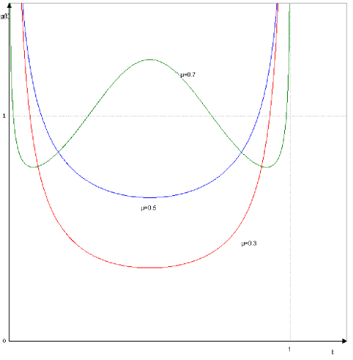
Figure 1: The density function $g$ of $A$, for several values of $\mu$.

Remark 3.2.

Similar discussions have been made in [4] in the framework of a skew Bessel process with dimension $2-2\alpha$ and skewness parameter $p$. Formula (20) is a particular case of formula in [4] for the density of the time spent positive (called $f_{p,\alpha}$ in [4]).

3.3 The case of many stable (1/2) variables

In this Subsection, we consider again $n$ iid stable (1/2) variables, i.e.: $T_{1},\ldots,T_{n}$, and we will study the distribution of:

$$A^{(1)}_{1}=\frac{T_{1}}{T_{1}+\ldots+T_{n}}\ .$$ (21)

The following Theorem answers to an open question (and even in a more general sense) stated at the end of [9].

Theorem 3.3.

The density function of the random variable $A^{(1)}_{1}$ is given by:

$$P\left(A^{(1)}_{1}\in dz\right)=\frac{1}{\pi}\frac{dz}{\sqrt{z}\sqrt{1-z}\left[(n-1)z+\frac{1}{n-1}\left(1-z\right)\right]}\ ,\ \ z\in[0,1].$$ (22)

Proof of Theorem 3.3.
We first remark that, with $C$ denoting a standard Cauchy variable, using e.g. (2):

$$A^{(1)}_{1}\stackrel{{\scriptstyle(law)}}{{=}}\frac{T_{1}}{T_{1}+(n-1)^{2}T_{2}}\stackrel{{\scriptstyle(law)}}{{=}}\frac{1}{1+(n-1)^{2}C^{2}}\ .$$ (23)

Hence, with $f$ standing again for a test function, and invoking the density of a standard Cauchy variable, that is: for every $x\in\mathbb{R}$, $g(x)=\frac{1}{\pi(1+x^{2})}$ we have:

$$E\left[f\left(A^{(1)}_{1}\right)\right] = E\left[f\left(\frac{1}{1+(n-1)^{2}C^{2}}\right)\right]$$

$$= \frac{1}{\pi}\ \int^{\infty}_{-\infty}\frac{dx}{1+x^{2}}\ f\left(\frac{1}{1+(n-1)^{2}x^{2}}\right)$$

$$\stackrel{{\scriptstyle x^{2}=y}}{{=}} \frac{2}{\pi}\ \int^{\infty}_{0}\frac{dy}{2\sqrt{y}(1+y)}\ f\left(\frac{1}{1+(n-1)^{2}y}\right)$$

Changing the variables $z=\frac{1}{1+(n-1)^{2}y}$, we deduce:

$$E\left[f\left(A^{(1)}_{1}\right)\right]=\frac{1}{\pi}\ \int^{1}_{0}\frac{dz}{(n-1)^{2}z^{2}}\ \frac{(n-1)\sqrt{z}}{\sqrt{z-1}\left(1+\frac{1}{(n-1)^{2}}\left(\frac{1}{z}-1\right)\right)}\ f\left(z\right),$$

and (22) follows easily.     

Figure 2 presents the plot of the density function $h$ of $A^{(1)}_{1}$, for several values of $n$.

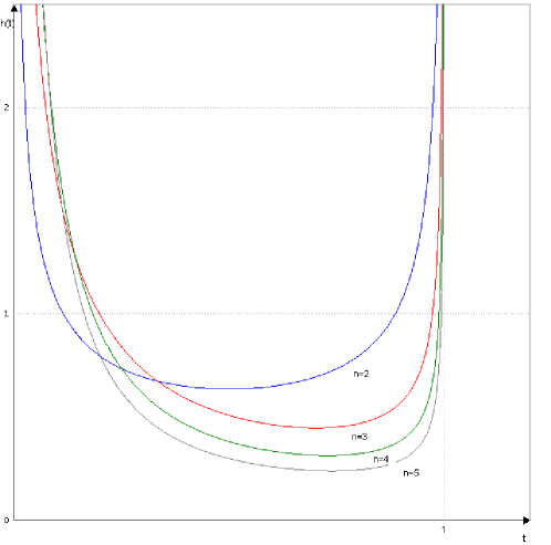
Figure 2: The density function $h$ of $A^{(1)}_{1}$, for several values of $n$.

Corollary 3.4.

The following convergence in law holds:

$$n^{2}A^{(1)}_{1}(n)\overset{{(law)}}{\underset{n\rightarrow\infty}{\longrightarrow}}C^{2}\ .$$ (24)

Proof of Corollary 3.4.
It follows from Theorem 3.3 by simply remarking that $C\stackrel{{\scriptstyle(law)}}{{=}}C^{-1}$. Hence:

$$n^{2}A^{(1)}_{1}(n)=\frac{n^{2}}{1+(n-1)^{2}C^{2}}=\frac{1}{\frac{1}{n^{2}}+\left(\frac{n-1}{n}\right)^{2}C^{2}}\stackrel{{\scriptstyle n\rightarrow\infty}}{{\longrightarrow}}\frac{1}{C^{2}}\stackrel{{\scriptstyle(law)}}{{=}}C^{2}.$$

   

4 Conclusion and comments

We end up this article with some comments: usually, a scaling argument is "one-dimensional", as it involves a time-change. Exceptionally (or so it seems to the authors), here we could apply a scaling argument in a multivariate framework. We insist that the scaling Lemma plays a key role in our proof. The curious reader should also look at the totally different proof of this Theorem in [2], which mixes excursion theory and the Feynman-Kac method.

Acknowledgements
The author S. Vakeroudis is very grateful to Professor R.A. Doney for the invitation at the University of Manchester as a Post Doc fellow where he prepared a part of this work.

References

- [1] M.T. Barlow, J.W. Pitman and M. Yor (1989). On Walsh’s Brownian motion. Sém. Prob. XXIII, Lect. Notes in Math., 1372, Springer, Berlin Heidelberg New York, pp. 275-293.
- [2] M.T. Barlow, J.W. Pitman and M. Yor (1989). Une extension multidimensionnelle de la loi de l’arc sinus. Sém. Prob. XXIII, Lect. Notes in Math., 1372, Springer, Berlin Heidelberg New York, pp. 294-314.
- [3] L. Chaumont and M. Yor (2012). Exercises in Probability: A Guided Tour from Measure Theory to Random Processes, via Conditioning. Cambridge University Press, 2nd Edition.
- [4] Y. Kasahara and Y. Yano (2005). On a generalized arc-sine law for onedimensional diffusion processes. Osaka J. Math., 42, pp. 1-10.
- [5] J. Lamperti (1958). An occupation time theorem for a class of stochastic processes. Trans. Amer. Math. Soc., 88, pp. 380-387.
- [6] P. L vy (1939). Sur un probl me de M. Marcinkiewicz. C.R.A.S., 208, pp. 318-321. Errata p. 776.
- [7] P. L vy (1939). Sur certains processus stochastiques homog nes. Compositio Math., t. 7, pp. 283-339.
- [8] H.P. McKean (1975). Brownian local time. Adv. Math., 16, pp. 91-111.
- [9] V.G. Papanicolaou, E.G. Papageorgiou and D.C. Lepipas (2012). Random Motion on Simple Graphs. Methodol. Comput. Appl. Probab., 14, pp. 285-297.
- [10] J.B. Walsh (1978). A diffusion with discontinuous local time. Ast risque, 52-53, pp. 37-45.
- [11] S. Watanabe (1995). Generalized arc-sine laws for one-dimensional diffusion processes and random walks. Proc. Sympos. Pure Math., 57, Stoch. Analysis, Cornell University (1993), Amer. Math. Soc., pp. 157-172.
- [12] D. Williams (1969). Markov properties of Brownian local time. Bul. Am. Math. Soc., 76, pp. 1035-1036.
- [13] M. Yor (1995). Local times and Excursions for Brownian motion: a concise introduction. Lecciones en Mathematicas Universidad Central de Venezuela, Caracas.
- [14] V.M. Zolotarev (1957). Mellin-Stieltjes transforms in probability theory. Teor. Veroyatnost. i Primenen., 2, pp. 444-469.
- [15] V.M. Zolotarev (1994). On the representation of the densities of stable laws by special functions. (In Russian.) Teor. Veroyatnost. i Primenen., 39, no. 2, pp. 429-437; translation in Theory Probab. Appl., (1995) 39, no. 2, pp. 354-362.