A Uniformly Selected Sample of Low-mass Black Holes in Seyfert 1 Galaxies

Abstract

We have conducted a systematic search of low-mass black holes (BHs) in active galactic nuclei (AGNs) with broad H$\alpha$ emission lines, aiming at building a homogeneous sample that is more complete than previous ones for fainter, less highly accreting sources. For this purpose, we developed a set of elaborate, automated selection procedures and applied it uniformly to the Fourth Data Release of the Sloan Digital Sky Survey. Special attention is given to AGN–galaxy spectral decomposition and emission-line deblending. We define a sample of 309 type 1 AGNs with BH masses in the range $8\times 10^{4}$–$2\times 10^{6}$ $M_{\odot}$ (with a median of $1.2\times 10^{6}$ $M_{\odot}$), using the virial mass estimator based on the broad H$\alpha$ line. About half of our sample of low-mass BHs differs from that of Greene & Ho, with 61 of them discovered here for the first time. Our new sample picks up more AGNs with low accretion rates: the Eddington ratios of the present sample range from $\lesssim 0.01$ to $\sim 1$, with 30% below $0.1$. This suggests that a significant fraction of low-mass BHs in the local Universe are accreting at low rates. The host galaxies of the low-mass BHs have luminosities similar to those of $L^{*}$ field galaxies, optical colors of Sbc spirals, and stellar spectral features consistent with a continuous star formation history with a mean stellar age of less than 1 Gyr.

1 Introduction

Supermassive black holes (BHs) with masses $M_{\mathrm{BH}}\gtrsim 10^{6}$ $M_{\odot}$ reside in the centers of galaxies with a spheroidal stellar component. Although their formation mechanisms are still not well understood, correlations of their masses with the host galaxy properties have been fairly well established (Magorrian et al. 1998; Gebhardt et al. 2000; Ferrarese & Merritt 2000). However, far less is known about lower mass BHs in the regime $M_{\mathrm{BH}}$ $\approx 10^{3}-10^{6}$ $M_{\odot}$, the so-called intermediate-mass BHs, presumably hosted by smaller stellar systems such as dense star clusters and late-type or dwarf galaxies (see, e.g., van der Marel 2004 for a review). Intermediate-mass BHs are important for studies of BH formation and growth, galaxy formation and evolution, and active galactic nuclei (AGNs). In current models of galaxy evolution in a hierarchical cosmology, supermassive BHs must have been built up from accretion onto much smaller “seeds,” in conjunction with merging with other BHs. These models also predict that smaller-scale structures form at later times (cosmic “downsizing”), and one might expect that seed BHs in smaller stellar systems may not have had enough time to be fully grown. A population of intermediate-mass BHs likely exists in the local Universe. The mass function of the present-day intermediate-mass BHs and their host galaxy properties can be used to discriminate between different models for seed BHs and help shed light on the coevolution of BHs and galaxies (e.g., Volonteri et al. 2008).

Searching for intermediate-mass BHs by direct, dynamical measurements turns out to be a difficult task. The gravitational sphere of influence of these objects cannot be resolved using current facilities, except for a handful of the nearest ($\lesssim 1$ Mpc) star clusters and galaxies. A practicable approach is to search, through optical spectroscopic surveys, for those BHs that are actively accreting and thus revealing themselves as AGNs, for which their virial masses can be estimated using the empirical relations using emission-line width and luminosity (e.g., Kaspi et al. 2000; Greene & Ho 2005b). A prototype of such a kind of AGN is the Seyfert nucleus residing in the nearby dwarf spiral (Sdm) galaxy NGC 4395 (Filippenko & Ho 2003), which has a BH mass $3.6\pm 1.1\times 10^{5}$ $M_{\odot}$ as measured via reverberation mapping observations of the C IV $\lambda 1549$ line (Peterson et al. 2005). Using spectroscopic data from the Sloan Digital Sky Survey (SDSS; York et al. 2000) Greene & Ho (2004, 2007b) have conducted systematic searches for AGNs with intermediate-mass BHs, leading to the discovery of some 200 candidates. One noticeable feature of their sample is the overall relatively high Eddington ratios ($L\mathrm{{}_{bol}}/L\mathrm{{}_{Edd}}$) and a small number of objects with $L\mathrm{{}_{bol}}/L\mathrm{{}_{Edd}}<0.1$, a likely consequence of their strict criteria for detecting the broad H$\alpha$ line.

According to Greene & Ho (2007a), the space density of massive BHs in AGNs decreases toward the low-mass end ($M_{\mathrm{BH}}\lesssim 2\times 10^{6}$ $M_{\odot}$). This may imply that intermediate-mass BHs are truly rare, or their AGN phase has a short duty cycle. The former may be due either to the decreasing bulge fraction in small galaxies and/or to an existing lower limit on the possible mass of nuclear BHs (see, e.g., Haehnelt et al. 1998). From the standpoint of observations, however, it is plausible that the apparent paucity may just be a selection effect. This is because low-mass AGNs radiate at low luminosities, even if they are shining at their maximum rate, and, even worse, detection of their continuum and line emission is often susceptible to dilution by starlight of the host galaxy due to the limited spatial resolution of observations. This may explain the dearth of low-mass AGNs with $L\mathrm{{}_{bol}}/L\mathrm{{}_{Edd}}<0.1$ in the sample of Greene & Ho (2007a), who adopted very strict selection criteria for detecting broad emission lines. After all, low-mass AGNs with low accretion rates do exist. Depending on the adopted BH mass, NGC 4395 has $L\mathrm{{}_{bol}}/L\mathrm{{}_{Edd}}$ $\approx 0.002-0.02$ (Filippenko & Ho 2003; Peterson et al. 2005), and low Eddington ratios have been reported for smaller samples of low-mass BHs in late-type galaxies based on infrared (Satyapal et al. 2008) and X-ray (Desroches & Ho 2009) observations.

The above considerations suggest that it is desirable to compile a more complete, homogeneous sample of low-mass AGNs, with emphasis on enlarging the number of systems with low accretion. This would result in a less biased distribution of accretion rates (as represented by $L\mathrm{{}_{bol}}/L\mathrm{{}_{Edd}}$), which is important for a more complete picture of BH demographics (e.g., Schulze & Wisotzki 2010). Moreover, low-$L\mathrm{{}_{bol}}/L\mathrm{{}_{Edd}}$, low-mass BHs are interesting in and of themselves for AGN research, as they extend the dynamic range of physical variables to extreme values.

Optical spectroscopy is a powerful means of estimating BH masses for AGNs on a large scale. However, like the proverbial finding a needle in a haystack, searching for low-mass AGNs with low $L\mathrm{{}_{bol}}/L\mathrm{{}_{Edd}}$ in the SDSS database is rather challenging, since their spectra within the 3″-diameter fiber aperture are generally dominated by starlight from the host galaxies. To recover the weak broad H$\alpha$ line, the strongest permitted line in the optical region on which we base our BH mass estimation, requires two essential steps—accurate decomposition of AGN-starlight spectra and careful deblending of the broad H$\alpha$ component from its associated narrow lines (narrow H$\alpha$ and the [N II] $\lambda\lambda 6548,6583$ doublet). Equally important is to design carefully both a set of broad-line criteria and an automated selection procedure to mine effectively the huge volume data set.

In this paper we present a sample of 309 Seyfert 1 galaxies hosting a central BH of $M_{\mathrm{BH}}<2\times 10^{6}$ $M_{\odot}$, uniformly selected from the fourth data release (DR4; Adelman-McCarthy et al. 2006) of the SDSS. We have carefully designed selection criteria and spectral fitting methods aimed at detecting low-mass BHs with relatively weak emission lines. Their Eddington ratios are found to range from $\lesssim 0.01$ to $\sim 1$, with 30% of the objects having $L\mathrm{{}_{bol}}/L\mathrm{{}_{Edd}}<0.1$. The spectral fitting method is described in Section 2, and the selection criteria and sample construction in Section 3. Results of the spectral and imaging analyses are presented in Section 4, followed by a summary in Section 5. We use a cosmology with $H_{0}=70$ $\mathrm{km~{}s^{-1}}$ Mpc^-1, $\Omega_{m}=0.3$, and $\Omega_{\Lambda}=0.7$.

2 Data and Processing Methods

This section describes several technical aspects of our procedure for mining the SDSS spectroscopic data to construct the low-mass AGN sample, mainly concerning continuum and emission-line fitting and assessment of the uncertainties of derived parameters. As our data reduction and analysis methods are largely shaped by the characteristics of the SDSS data, we first give a brief description of the SDSS data (see Stoughton et al. 2002 for details).

2.1 SDSS Data

The SDSS is an imaging and spectroscopic survey, using a dedicated 2.5-m telescope to image one-quarter of the sky and to perform follow-up spectroscopic observations. The imaging data were collected in a drift-scan mode in five bandpasses ($u$, $g$, $r$, $i$, and $z$) on nights of pristine conditions. The photometric calibration is accurate to 5%, 3%, 3%, 3%, and 5%, respectively. Targets for spectroscopy were selected based on the photometric data. Galaxy candidates were targeted as resolved sources with $r$-band Petrosian magnitudes $<17.77$; luminous red galaxy candidates were specifically targeted by two different sets of criteria with $r$-band Petrosian magnitude $<19.2$ and 19.5, respectively; low-redshift quasar candidates were selected according to a set of color criteria with $i$-band PSF magnitude $<19.1$; high-redshift quasar candidates were selected according to a different set of color criteria with $i$-band PSF magnitude $<20.2$. Also targeted were unresolved objects with radio counterparts detected by the FIRST survey (Becker et al. 1995), partial objects with X-ray counterparts detected by ROSAT (Voges et al. 1999) and other serendipitous sources when free fibers were available on a plate. Fibers that feed the SDSS spectrographs subtend a diameter of 3″ on the sky, which corresponds to 6.5 kpc at $z=0.1$. The nominal total exposure time for each plate is 45 minutes, which typically yields a signal-to-noise ratio (S/N) of 4.5 pixel^-1 for objects with a $g$-band magnitude of 20.2. The spectra are flux- and wavelength-calibrated, with 4096 pixels from 3800 to 9200 Å at a resolution $R\equiv\lambda/\Delta\lambda\approx 1800$. Redshifts are determined with pipeline code (spectro1d) by either cross-correlating the spectra with templates or measuring emission lines; for galaxies, the typical redshift accuracy is about $30$ $\mathrm{km~{}s^{-1}}$. spectro1d also automatically classifies the spectra into quasars, galaxies, stars, or unknown.

We correct the SDSS spectra for Galactic extinction using the extinction map of Schlegel et al. (1998) and the reddening curve of Fitzpatrick (1999), and initially transform them into the rest frame using the redshifts provided by the SDSS pipeline.

2.2 Continuum and Emission-line Fitting

We summarize the procedures to model the continua and emission-line profiles, as well as several updates to our previous treatments. The fits are implemented with Interactive Data Language (IDL) and based on the MPFIT package (Markwardt 2009), which performs $\chi^{2}$-minimization using the Levenberg–Marquardt technique.

Taken within a 3″-diameter aperture, many SDSS spectra have a significant contribution from host galaxy starlight. Careful removal of starlight, especially stellar absorption features, is essential for the detection and accurate measurement of possible AGN emission lines (see Ho et al. 1997a and Ho 2004 for detailed discussions). For this purpose, a set of algorithms has been developed; we refer readers to Zhou et al. (2006) for details, and only stress here two key issues with updates.

• Host galaxy starlight is modeled with six synthesized galaxy spectral templates, which were built from the library of simple stellar populations of Bruzual & Charlot (2003) using the Ensemble Learning Independent Component Analysis algorithm (Lu et al. 2006). The templates are broadened by convolution with a Gaussian to match the stellar velocity dispersion of the host galaxy. Particularly, to account for possible errors in the redshifts provided by the SDSS pipeline, we loop possible redshifts near the SDSS value by shifting the starlight model in adaptive steps; the fit with minimum reduced $\chi^{2}$ is adopted as the final result. This is important to the measurement of host galaxy velocity dispersion and weak emission lines.

• The optical Fe II emission is modeled with two separate sets of templates in analytical form, one for the broad-line system and the other for the narrow-line system. These two sets of templates are constructed from measurements of I Zw 1 by Véron-Cetty et al. (2004), as listed in their Tables A1 and A2; see Dong et al. (2008) for details, and Dong et al. (2011) for tests of the Fe II modeling. The analytical form enables us to fit Fe II multiplets of any width. This is especially useful in the case of low-mass AGNs, which often have Fe II lines significantly narrower than those of I Zw 1, from which almost all existing empirical Fe II templates have been built (cf. Greene & Ho 2007b).

During the fitting two kinds of spectral regions had been masked out: bad pixels as flagged by the SDSS pipeline and wavelength ranges that are seriously affected by prominent emission lines.

In some AGN-dominated spectra where the starlight contribution is insignificant, the broad lines are so strong and broad that most of the continuum and Fe II regions would be masked out as emission-line regions using the above continuum-fitting method (see Zhou et al. 2006). In practice such AGN-dominated sources have undetectable Ca II K (3934 Å), Ca II H + H$\epsilon$ (3970 Å), and H$\delta$ (4102 Å) absorption features (see the Appendix of Dong et al. 2011). For these cases we fit simultaneously the nuclear continuum, the Fe II multiplets, and other emission lines (see Dong et al. 2008 for details). We recalculate the reduced $\chi^{2}$ of the fits around the H$\alpha$ and H$\beta$ regions. Spectra with the reduced $\chi^{2}>1.1$ in either region are subjected for further refined fitting of the line profiles.

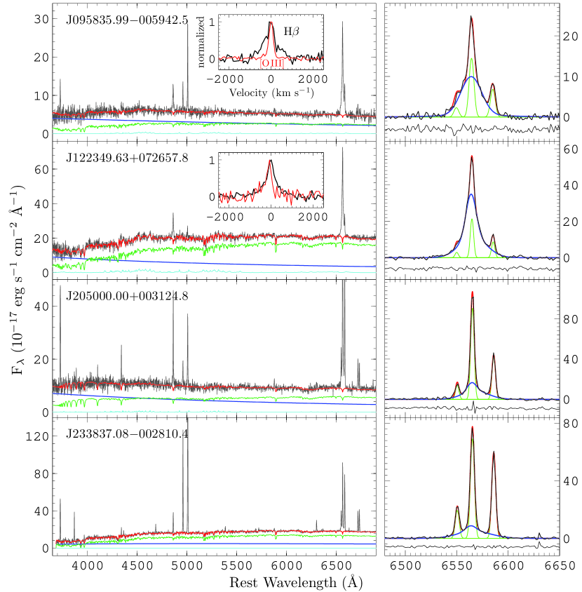
Figure 1: Illustration of the continuum and emission-line fittings for four low-accretion, low-mass Seyfert 1s that are not included in the Greene & Ho (2007b) sample. Left: Observed SDSS spectrum (black), the total model (red), the decomposed components of the host galaxy (green), the AGN continuum (blue), and the Fe II multiplet emission (cyan). The inset is a zoomed-in view of a comparison of the H$\beta$ line (black) and the [O III] $\lambda 5007$ line profile (ref) in the velocity space ($x$-axis), both with the continuum subtracted and the peak flux density normalized at unity. Right: Emission-line profile fitting in the H$\alpha$ $+$ [N II] region.

The emission-line profiles, particularly the H$\alpha$ + [N II] complex (or H$\alpha$ + [N II] + [S II] if H$\alpha$ is very broad), are fitted using the code described in detail in Dong et al. (2005). We fit the emission lines using various schemes, and the one with the minimum reduced $\chi^{2}$ is adopted as the final result. Basically, each emission line (narrow or broad) is fitted incrementally with as many Gaussians as statistically justified. The statistical criteria we adopt for convergence (i.e., tolerance threshold) is that either the reduced $\chi^{2}\leq 1.1$ or the fit cannot be improved significantly by adding in one more Gaussian with a chance probability less than 0.05 according to $F$-test. We show some examples of the fits in Figure 1.

2.3 Error Assessment for Emission-line Parameters

The parameters of the emission lines, both narrow and broad, are measured from their best-fitting multi-Gaussian models. For broad lines, the measurement uncertainties of the line parameters arise from statistical noise, continuum subtraction (i.e., starlight, AGN (pseudo-)continuum, or both), and subtraction of nearby narrow lines. Formally, the total error is the quadrature sum of the three independent terms,

$$\sigma^{2}_{\rm total}=\sigma^{2}_{\rm n}+\sigma^{2}_{\rm cont\_sub}+\sigma^{2}_{\rm NL\_sub}~{}.$$ (1)

The measurement uncertainty due to statistical noise, $\sigma_{\rm n}$, is given by the fitting code MPFIT. In practice, the error term caused by possible mismatch of the continuum models is hard to estimate for every spectrum. For each of our low-mass AGN spectra, we visually inspect the continuum subtraction to guarantee that the subtraction uncertainty is at least much below the 1 $\sigma$ spectral flux density error; in particular, we carefully check the higher-order Balmer absorption lines in the cases where there is considerable contribution from intermediate-aged stellar populations. On the other hand, in low-mass AGN spectra the broad Balmer lines are relatively narrow, and, just like the narrow lines, their measurement is little affected by the placement of the large-scale continuum (see Section 2.5 of Dong et al. 2008). This is particularly true for broad H$\alpha$ emission, because for intermediate-aged stellar populations the H$\alpha$ absorption feature is generally much weaker than H$\beta$ and other higher-order lines (e.g., up to H$\epsilon$). Hence, we believe that the $\sigma^{2}_{\rm cont\_sub}$ term has been well minimized and is negligible as far as the broad H$\alpha$ lines are concerned in this study (cf. Footnote 7 below).

As for the error term caused by the narrow line subtraction, its relative significance depends on the width of the broad H$\alpha$ line. In the case of very broad H$\alpha$, so broad that in the line profile inflections can be apparently seen in between the broad component and surrounding narrow lines, this term should be small and negligible. For a broad H$\alpha$ line that is both narrow and weak, this term may be significant, as the line deblending is highly dependent on the narrow-line model. We estimate it as follows. As described in Section 3.2 below, in the refined line-fitting stage we have four sets of fitting results out of the four schemes that adopt different narrow-line models. By using the $F$-test, we pick up the $n$ sets of fitting results that are worse than the best-fitting set with a chance probability greater than 0.1, and then calculate the error term for parameter $p$ as

$$\sigma_{\rm NL\_sub}=\sqrt{\frac{\sum_{i=1}^{n}(p_{i}-p_{\rm best})^{2}}{n}}~{}.$$ (3)

Our analysis indicates that the mean statistical relative error for the broad H$\alpha$ fluxes is 4%, and that the mean total relative error is 20%. For the FWHM of broad H$\alpha$, the mean statistical relative error is 7%, and the total relative error is 28%. In what follows, when we speak of the significance of the detection of a broad H$\alpha$ line (say, at the 3 $\sigma$ level), we mean its relative flux with respect to the statistical error ($\sigma_{\rm n}$); when we refer to the S/N of broad H$\alpha$, we mean the ratio of its flux to the total error ($\sigma_{\rm total}$).

3 Sample Construction

We start with the 451,000 spectra classified by the SDSS spectroscopic pipeline as “galaxy” or “QSO” at $z<0.35$ in the SDSS DR4 (444,465 “galaxies” and 6,535 “QSOs”, with duplicate observations counted). They were arrayed on 1052 plates of 640 fibers each, with a total spectroscopic sky coverage of 4783 deg² (Adelman-McCarthy et al. 2006). We set the redshift limit so that the H$\alpha$ line lies within the SDSS spectral coverage. To all the spectra we performed the continuum and emission-line fittings with the methods described in Section 2. Based on the fitting results, we first compile a parent sample of 8862 broad-line (type 1) AGNs according to our carefully defined criteria for detecting broad H$\alpha$ emission (Section 3.1), by using an automated selection procedure (Section 3.2). We then estimate the BH mass from the luminosity and width of the broad H$\alpha$ line using the formalism developed by Greene & Ho (2007b). Applying a high mass cut-off at $M_{\mathrm{BH}}=2\times 10^{6}$ $M_{\odot}$, we end up with a low-mass BH sample consisting of 309 sources.

In statistical studies of this nature, it is important to consider the impact of selection effects. Optimally, sample selection should be objective and clearly defined with quantitative criteria that are sufficiently reliable to select bona fide sources and, at the same time, sufficiently efficient to make the sample as complete as possible. Moreover, the criteria should be designed in such a way that it is easy to implement—usually through Monte Carlo simulations—corrections for selection effects (see, e.g., Hao et al. 2005; Greene & Ho 2007a; Lu et al. 2010). In addition to having well-defined and robust criteria, in practice an efficient, automated selection procedure is also required to handle large-volume data sets such as that from SDSS. We have made a concerted effort to design an efficient and effective selection procedure for these purposes.

3.1 Criteria for Detecting Broad H$\alpha$ Emission

The broad H$\alpha$ line is generally the strongest broad line in the optical spectra of AGNs. When it is weak, as expected in low-mass AGNs with low accretion rates, defining the criteria for broad H$\alpha$ detection is by no means trivial (see, e.g., Ho et al. 1997b; Greene & Ho 2004; Dong et al. 2005; Hao et al. 2005; Zhou et al. 2006; Greene & Ho 2007a, 2007b). For the purpose of comparison, we summarize some of the criteria adopted previously in the literature. In the early efforts to mine broad-line AGNs from the SDSS Early Data Release, Dong et al. (2005) used a simple criterion for the detection of broad H$\alpha$, by requiring that its S/N be $\geq 5$. Later, Zhou et al. (2006) used a stricter criterion, requiring the S/N of broad H$\alpha$ to be $\geq 10$ to select narrow-line Seyfert 1s. Greene & Ho (2007a) took a two-step procedure to select broad-line AGNs (see also Greene & Ho [2004] for a qualitative description of an earlier version of their criteria). In the first step, they employed an initial selection algorithm to select candidates with excess rms deviation in the H$\alpha$ region. In the second step, they performed detailed line-profile fitting of the H$\alpha$ + [N II] region, and set the broad H$\alpha$ criteria as,
(1) $\chi_{\rm N}^{2}/\chi_{\rm B}^{2}~{}>~{}1.2$,
(2) Flux(total H$\alpha$) / rms $~{}>~{}200$ Å, and
(3) EW(total H$\alpha$) $~{}>~{}15$ Å,
where $\chi_{\rm B}^{2}$ and $\chi_{\rm N}^{2}$ represent the $\chi^{2}$ of the fits with and without accounting for broad H$\alpha$, respectively, and rms represents the rms deviations in the $6400-6700$ Å region of the continuum-subtracted spectra. Criterion 1 requires that adding a broad H$\alpha$ component to the fit results in a 20% decrease in $\chi^{2}$; this empirical rule is inspired by $F$-test statistics used to evaluate the significance of line fits (Hao et al. 2005). Criteria 2 and 3 are aggressive cuts (their “detection threshold”) to guarantee the reliability of BH mass estimates based on broad H$\alpha$ line width and luminosity. As the detection threshold is quite strict, the low-mass ($M_{\mathrm{BH}}<2\times 10^{6}$ $M_{\odot}$) AGN sample tends to have rather high Eddington ratios ($L\mathrm{{}_{bol}}/L\mathrm{{}_{Edd}}>0.1$ mostly; see Figure 1 of Greene & Ho 2007b). In an effort to find more low-$L\mathrm{{}_{bol}}/L\mathrm{{}_{Edd}}$ objects, Greene & Ho (2007b) manually selected additional sources and tagged them as candidate low-mass systems (their $c$ subsample).

In this work, we select broad-line AGNs based directly on the results of the emission-line fits. Our broad H$\alpha$ criteria are the following:
(1) $P_{F-{\rm test}}<0.05$,
(2) Flux(H$\alpha^{\rm B}$) $>10^{-16}$ erg s^-1 cm^-2,
(3) S/N(H$\alpha^{\rm B}$) $\geq 5$, and
(4) $h_{\rm B}\geq 2$ rms,
where $P_{F-{\rm test}}$ is the chance probability given by the $F$-test that adding a broad H$\alpha$ in the model is significant; S/N(H$\alpha^{\rm B}$) $=$ Flux(H$\alpha^{\rm B}$)$/\sigma_{\rm total}$, as stated in Section 2.3; $h_{\rm B}$ is the height of the best-fit broad H$\alpha$ line; and rms is the rms deviation of the continuum-subtracted spectra in the emission-line–free region near H$\alpha$. Criterion 1 gives the statistical significance of detecting broad H$\alpha$ given by $F$-test (see Footnote 3). The lower limit of the broad H$\alpha$ flux in Criterion 2 is set to eliminate possible spurious detections caused by systematic errors, such as those caused by inappropriate continuum subtraction (cf. Footnote 7). Criterion 3 is to ensure the reliability of broad H$\alpha$ in terms of S/N. Criterion 4 minimizes spurious detections mimicked by narrow-line wings or any large-scale fluctuation in the continuum; it is set by trial-and-error based on the confirmation of the AGN nature in some of the objects by the presence of broad H$\beta$  or by our long-slit observations using the MMT 6.5-m telescope with a narrow slit width under good seeing conditions. Our final results are not very sensitive to the exact value chosen for the $h_{\rm B}$ threshold; changing the value by $\pm$10% has little impact on final results. The S/N threshold in Criterion 3 generally selects objects with $h_{\rm B}$ much larger than 2 rms.

3.2 The Automated Selection Procedure

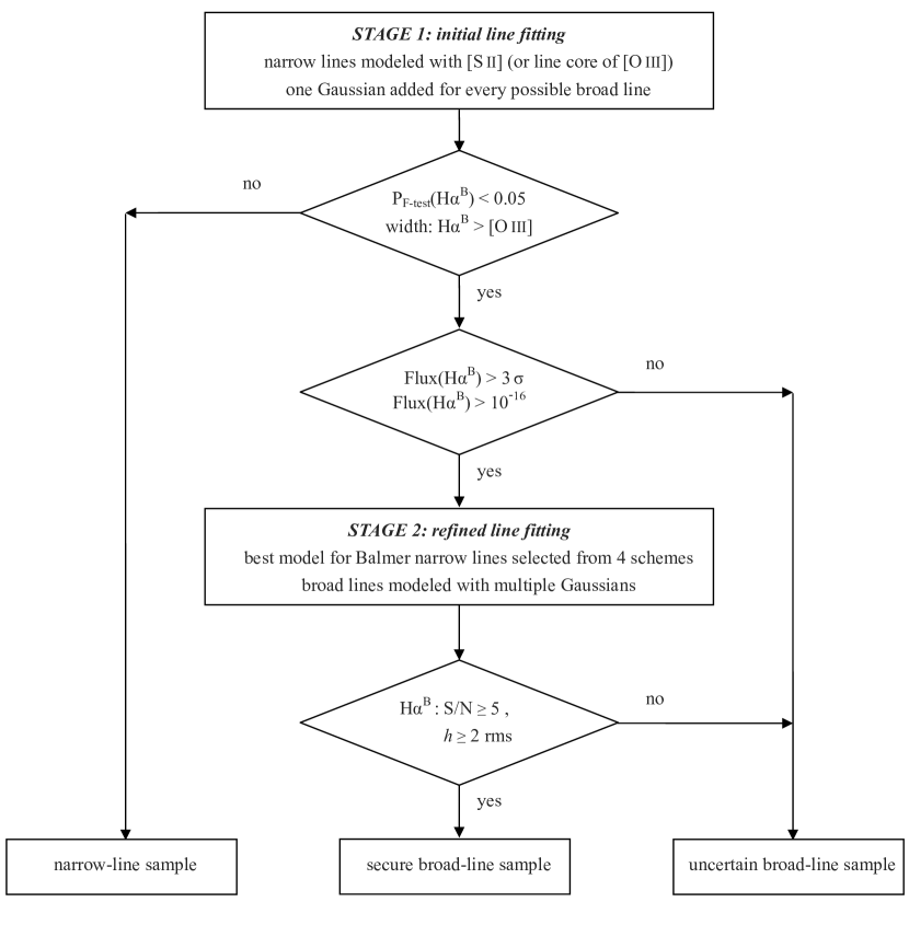
Figure 2: Flow chat of the automated procedure to select objects with the broad H$\alpha$ line. See Section 3 for details.

The selection procedure is composed of two stages. In the initial fitting stage, each spectrum is fitted quickly, with the aim of reducing the number of broad H$\alpha$ candidates passed to the second stage. Next, the H$\alpha$ $+$ [N II] complex (or H$\alpha$ $+$ [N II] $+$ [S II] if H$\alpha$ is very broad) is fitted carefully to get reliable parameters for broad H$\alpha$. We then select bona fide broad H$\alpha$ emitters based on the criteria outlined above. We describe these two stages in detail; a flow chart is given in Figure 2.

The initial stage has three steps. The first is to build a narrow-line model from the [S II] $\lambda\lambda 6716,6731$ doublet (or the core component of the [O III] $\lambda\lambda 4959,5007$ doublet if [S II] is weak). The two [S II] lines are assumed to have the same profile and are fixed in separation by their laboratory wavelengths. Each line is fitted with one Gaussian, and, if either is detected at S/N $\geq 10$, more Gaussians are added. The final fit is achieved following the tolerance threshold as stated in Section 2.2. The [O III] doublet is fitted in a similar way. The flux ratio of the doublet $\lambda$5007/$\lambda$4959 is fixed to the theoretical value of 2.98. The [O III] profile usually shows a broad wing blueward of the line core (e.g., Greene & Ho 2005a; Zhang et al. 2011); thus, it is fitted with multiple Gaussians, one for the line core, and one or more for the wings. In this way we build a model for the narrow-line profile, using the best-fit model for [S II] if we can, or the core of [O III] if the [S II] lines are too weak ($<5$ $\sigma$ significance).

Step 2 of the first stage is to fit the H$\alpha$ + [N II] region. The narrow H$\alpha$ component and the [N II] $\lambda\lambda 6548,6583$ doublet are modeled with the narrow-line model obtained above, assuming that these three lines have the same redshift and profile. The flux ratio of the [N II] doublet $\lambda$6583/$\lambda$6548 is fixed to the theoretical value of 2.96. An additional Gaussian to account for possible broad H$\alpha$ is added if the $\chi^{2}$ decreases significantly with a $F$-test probability $<$0.05. At this point the centroid of the broad component is fixed to that of narrow H$\alpha$, while the width and flux are left as free parameters.

In Step 3, a reduced number of objects with candidate broad H$\alpha$ are selected, which will be passed to the next stage. They are selected from those with a possible “broad” H$\alpha$ component determined from Step 2, which have (1) FWHM of the broad component greater than that of any narrow lines (particularly [O III] $\lambda 5007$); and (2) flux 3 times greater than the flux error given by MPFIT (namely $\sigma_{\rm n}$), and meanwhile greater than $10^{-16}$ erg s^-1 cm^-2. These criteria are physically meaningful and practical (see Section 3.1); in particular, we believe from our experiments that the sensitivity of detecting a broad H$\alpha$ line in the general SDSS database is greater than $\sim 10^{-16}$ erg s^-1 cm^-2. 

The initial stage of line fitting produced $\sim$49,600 spectra (11%) that appear to have a “broad” H$\alpha$ component that is statistically significant according to the $F$-test (Step 2), of which about 23,700 are regarded as physically reasonable candidates (after Step 3). These candidates are passed to the second stage for refined fitting of their emission-line profiles.

The final fits are performed using different schemes for modeling the narrow H$\alpha$ line. Since narrow H$\alpha$ (and H$\beta$) line can arise from emitting regions with a larger range of density and ionization than forbidden lines such as [N II] and [S II], it may have a different profile than [S II] (see Section 2 of Ho et al. 1997b for details; also Zhang et al. 2008). Considering this fact, we employ four different models for treating narrow H$\alpha$: (1) a single-Gaussian model built from narrow H$\beta$, if broad H$\beta$ is not detected in the first stage and narrow H$\beta$ can be fitted well with one Gaussian; (2) a model built from the best-fit [S II] with one or more Gaussians, as described above; (3) a single-Gaussian model from the best-fit core component of [O III]; (4) a multiple-Gaussian model from the best-fit global profile of [O III]. In each scheme, the H$\alpha$ $+$ [N II] region is fitted in a similar way as in Step 2 of the first stage, except that the possible broad H$\alpha$ is now modeled with as many Gaussians as statistically justified (see Section 2.2), and the centroid of broad H$\alpha$ is no longer fixed. The fitting scheme that gives the smallest reduced $\chi^{2}$ is adopted as the final result. The bona fide broad-line AGNs are then selected based on the broad H$\alpha$ criteria described in Section 3.1.

Our analysis yielded a total of 8862 sources (with duplicates removed) with secure detections of broad H$\alpha$. These form our parent sample of broad-line AGNs (namely Seyfert 1s and quasars).

3.3 Low-mass AGN Sample

It has become possible since the last decade to estimate BH masses in type 1 AGNs using single-epoch spectra, thanks to the significant advances in the reverberation mapping experiments of nearby Seyfert galaxies and quasars (e.g., Kaspi et al. 2000; Peterson et al. 2004). In this paper, we adopt the $M_{\mathrm{BH}}$ formalism presented by Greene & Ho (2007b), which makes use of the luminosity and FWHM of the broad H$\alpha$ line (see their equation A1). This formalism is based on the radius-luminosity relation reported by Bentz et al. (2006) and assumes a spherical broad-line region (BLR) with a virial coefficient of $f=0.75$. For ease of comparison, we simply adopt the same upper limit on BH mass, $2\times 10^{6}M_{\odot}$, which Greene & Ho (2007b) used to define low-mass BHs. This threshold was motivated by the smallest nuclear BH that has been reliably measured dynamically, $M_{\mathrm{BH}}=2.5\times 10^{6}M_{\odot}$ in M32 (Verolme et al. 2002). This cut produces a final sample of 309 AGNs with low-mass BHs.

Note that Wang et al. (2009) re-calibrated the BH mass formalisms based on single-epoch broad H$\beta$ and Mg II $\lambda 2800$ lines, stressing the nonlinear relation between the virial velocity of the BLR clouds and the FWHMs of the single-epoch broad lines. This nonlinearity probably arises from the mixture of non-virial components in the total profile of broad emission lines in single-epoch spectra (see Section 4.2 of Wang et al. 2009 for detailed discussion, and also Collin et al. 2006 and Sulentic et al. 2006). The mass estimators of Wang et al. (2009), however, were calibrated using reverberation mapping data for AGNs with BHs in the mass range $10^{7}$ to $10^{9}$ $M_{\odot}$, which does not cover the low-mass regime studied in this paper. Considering the uncertainty in extrapolating the empirical relations to the lower $M_{\mathrm{BH}}$ end by more than an order of magnitude, as well as the ease of comparison with previous samples, we adopt the same mass formalism as used by Greene & Ho (2007b). Moreover, we point out that the non-virial components, if any, may be less significant in our sample of low-mass objects, whose broad H$\alpha$ lines tend to be roughly symmetrical and generally close to a Gaussian. The statistical uncertainty of the BH masses is 0.3 dex (1 $\sigma$; cf. Wang et al. 2009), which is dominated by the systematics of the virial method rather than statistical measurement errors (see Xiao et al. 2011 for a detailed analysis).

We estimate their bolometric luminosities and Eddington ratios in the same way as Greene & Ho (2007b). That is, we adopt $L_{\rm bol}=9.8~{}\lambda L_{\lambda}(5100$ Å) (McLure & Dunlop 2004), which is consistent with the broad-band SED of NGC 4395 (Moran et al. 1999), while $\lambda L_{\lambda}(5100$ Å) is calculated from the H$\alpha$ luminosity (Greene & Ho 2005b). The Eddington ratio ($L\mathrm{{}_{bol}}/L\mathrm{{}_{Edd}}$) is the ratios between the bolometric and Eddington luminosities. The Eddington luminosity ($L\mathrm{{}_{Edd}}$) is the maximum luminosity of the central BH powered by spherical accretion, at which the gravity acting on an electron–proton pair is balanced by the radiation pressure due to electron Thomson scattering; $L\mathrm{{}_{Edd}}=1.26\times 10^{38}$ ($M_{\mathrm{BH}}$/$M_{\odot}$) erg s^-1. Table 1 shows the basic properties of the sample; Table 2 lists measurements of the emission-line parameters; and Table 3 gives the luminosities and BH masses. The emission-line parameters are calculated from the best-fit models of the line profiles. The flux of the Fe II $\lambda 4570$ emission blend is integrated in the rest-frame wavelength range 4434–4684 Å. For all measured emission-line fluxes, we regard the values as reliable detections if they have greater than 3 $\sigma$ significance; otherwise, we adopt the 3 $\sigma$ error as an upper limit. The data and fitting parameters for the low-mass BH sample are available online for the decomposed spectral components (continuum, Fe II, and other emission lines).

Figure 3 shows the distributions of the luminosity and FWHM of broad H$\alpha$, $M_{\mathrm{BH}}$, and $L\mathrm{{}_{bol}}/L\mathrm{{}_{Edd}}$ for the low-mass BH sample, overplotted on contours of the parent sample of 8862 broad-line AGNs. We note that, in the $M_{\mathrm{BH}}$–$L\mathrm{{}_{bol}}/L\mathrm{{}_{Edd}}$ plane (left panel), the lack of AGNs in the large-$M_{\mathrm{BH}}$, large-$L\mathrm{{}_{bol}}/L\mathrm{{}_{Edd}}$ region (upper right corner) reflects cosmic downsizing of supermassive BH activity (see, e.g., Heckman et al. 2004), in the sense that toward lower redshifts AGN activity gets shifted from massive BHs to their lower-mass counterparts. The dearth of objects in the small-$M_{\mathrm{BH}}$, small-$L\mathrm{{}_{bol}}/L\mathrm{{}_{Edd}}$ region (lower left corner) reflects the selection effect due to host galaxy starlight contamination (i.e., the difficulty in detecting broad H$\alpha$; see Section 3). The lone outlier is SDSS J103234.85$+$650227.9 (NGC 3259), which has a very low redshift ($z=0.0057$). Its broad H$\alpha$ line was first revealed from a high-resolution, high-S/N spectrum taken with the 10-m Keck telescope; the central stellar velocity dispersion of the host galaxy is $43\pm 4$ $\mathrm{km~{}s^{-1}}$ (Barth et al. 2008).

3.4 Comparison with the Greene & Ho (2007a, 2007b) Samples

Since our study represents an independent effort to select low-mass AGNs from what is otherwise identical SDSS data, it is worthwhile to compare our sample with that of Greene & Ho (2007b). Of the 309 objects in our sample, 160 are not included in Greene & Ho (2007b), 85 are not in their parent broad-line AGN sample (Greene & Ho 2007a), and 61 are not in either Greene & Ho (2007a) or Greene & Ho (2007b). On the other hand, of the 229 objects in Greene & Ho (2007b), 11 are not in the official data set of SDSS DR4 (Fermilab version) but rather were taken from the reductions of D. Schlegel at Princeton (J. Greene 2010, private communications), 37 are not in our sample due to our broad-line selection criteria, and an additional 32 are not in our low-mass sample because the estimated $M_{\mathrm{BH}}$ exceeds the mass cut. In total, there are 149 objects in common between the two studies (65% of the entire sample of Greene & Ho [2007b] and 48% of this present sample).

In light of the considerable discrepancy in the number of objects between the two samples, we compare their distributions of redshift, broad H$\alpha$ luminosity and FWHM, $M_{\mathrm{BH}}$, and $L\mathrm{{}_{bol}}/L\mathrm{{}_{Edd}}$ (Table 4). The $L\mathrm{{}_{bol}}/L\mathrm{{}_{Edd}}$ distributions are shown in Figure 4. The distributions of redshift, broad H$\alpha$ luminosity and FWHM, and $M_{\mathrm{BH}}$ are similar (within 0.1 dex on average) between our sample and the entire low-mass BH sample of Greene & Ho (2007b; including the 55 candidates below their detection threshold that dominate the $L\mathrm{{}_{bol}}/L\mathrm{{}_{Edd}}<0.1$ population). The median $L\mathrm{{}_{bol}}/L\mathrm{{}_{Edd}}$ of the present sample is 0.2 dex lower than that of their entire sample. However, we notice that the $L\mathrm{{}_{bol}}/L\mathrm{{}_{Edd}}$ distribution of their entire sample is not smooth. The $L\mathrm{{}_{bol}}/L\mathrm{{}_{Edd}}$ distribution of their uniformly selected sample of 174 objects, however, is smoother; this suggests that manual selection may have introduced inhomogeneities into their sample (cf. Xiao et al. 2011). When only the two uniformly selected samples are considered, there is a more significant difference in the $L\mathrm{{}_{bol}}/L\mathrm{{}_{Edd}}$ distribution: our sample has a smaller median value ($-0.7$ dex vs. $-0.4$ dex, computed in the logarithm) and a larger standard deviation ($0.5$ dex vs. $0.3$ dex) compared to Greene & Ho (2007b). The $M_{\mathrm{BH}}$ distributions of the two uniformly selected samples are similar. Hence the difference in $L\mathrm{{}_{bol}}/L\mathrm{{}_{Edd}}$ is due to fainter broad H$\alpha$ emitters detected in our sample; it has more objects in the low-luminosity end, with a median luminosity of broad H$\alpha$ 0.3 dex lower than their uniformly selected sample (see Table 4 and Figure 9). While there are 17 (10%) objects with $L\mathrm{{}_{bol}}/L\mathrm{{}_{Edd}}\leqslant 0.1$ in the uniformly selected sample of Greene & Ho (2007b) (and 59 in total in their entire sample), 89 (30%) objects of our sample have $L\mathrm{{}_{bol}}/L\mathrm{{}_{Edd}}\leqslant 0.1$. Thus, our approach has the advantage of systematically selecting more low-mass AGNs at low accretion rates.

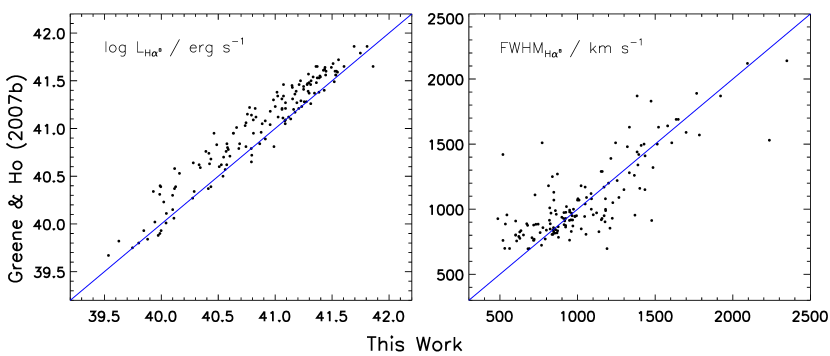
Figure 5: Comparison of the luminosities and FWHMs of broad H$\alpha$ for the 149 objects in common between our sample and that of Greene & Ho (2007b).

Since the spectral fitting methods adopted in this work are, in detail, different from those of Greene & Ho (2007b), we also compare the emission-line parameters derived from the two samples, using the 149 objects in common (Figure 5). The mean and standard deviation of the difference in the luminosity of broad H$\alpha$ (computed in logarithm) are 0.15 dex and 0.14 dex, respectively; for the FWHM of broad H$\alpha$, they are 0.02 dex and 0.09 dex, respectively. On average, the emission-line quantities of the two samples are consistent within 1 $\sigma$ dispersion (about 0.1 dex). The only noticeable exception is the broad H$\alpha$ luminosity, for which the values of Greene & Ho (2007b) are systematically higher than ours by 0.15 dex. After consulting with D. Schlegel (2011, private communications), we suspect that this systematic offset can be traced to differences in the calibration methods between the officially released SDSS data set we used and the Princeton version used by Greene & Ho (2007b). In any case, this calibration discrepancy is smaller than the difference between the two samples.

3.5 Supporting New Observations

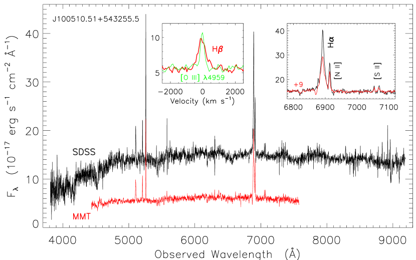
Figure 6: Demonstration of the spectra of a newly discovered Seyfert 1 galaxy with a low-mass BH and a low accretion rate, taken by the SDSS (black) and MMT (red), respectively. The inset on the left shows a zoomed-in view of the H$\beta$ line region in the MMT spectrum (without continuum subtraction), in direct comparison with the [O III] $\lambda 4959$ line profile in the velocity space ($x$-axis). The inset on the right shows a zoomed-in view of the H$\alpha$ $+$ [N II] $+$ [S II] region of the SDSS spectrum (black) and the MMT spectrum (red).

We have an ongoing program to observe a subsample of the nearby ($z<0.1$) low-mass BHs with the 6.5-m MMT telescope, using a 1″-wide slit under good seeing conditions. Compared to the SDSS spectra taken through 3″-diameter fibers, the contamination from the host galaxy starlight is significantly reduced in the MMT spectra. One of our goals is to check independently the reliability of the broad lines, particularly for the new objects that were not included in Greene & Ho (2007a, 2007b). The SDSS spectra of four such objects are shown in Figure 1; see also N. Jiang et al. (in preparation; their Figure 1) for SDSS J140040.56$-$015518.2 (UM 625; $L\mathrm{{}_{bol}}/L\mathrm{{}_{Edd}}=0.04$), which has extremely strong narrow emission lines, similar to NGC 4395 and POX 52. Here we show in Figure 6 the MMT spectrum of yet another object, SDSS J100510.51$+$543255.5. The broad H$\alpha$ component matches very well the one in the SDSS spectrum (see the right inset). Moreover, in the original MMT spectrum the H$\beta$ line already shows a profile significantly broader than the [O III] $\lambda 4959,5007$ doublet (see the left inset), even without subtracting the starlight. Hence the broad H$\beta$ component is real, definitely not an artifact caused by overestimating the H$\beta$ absorption in the starlight spectrum. As another independent check, we also obtained Chandra X-ray observations for four nearby objects with $L\mathrm{{}_{bol}}/L\mathrm{{}_{Edd}}<0.1$. We find that their X-ray emission is indeed weak up to 10 keV, consistent with the low $L\mathrm{{}_{bol}}/L\mathrm{{}_{Edd}}$ nature inferred from their optical spectra (W. Yuan et al., in preparation).

4 Sample Properties

As described in last section, the present sample and the previous one by Greene & Ho (2007b) share only about half of the objects in common. Moreover, the new sample spans a wider regime in the parameter space by including many more low-accretion systems. It is therefore of particular interest to investigate the ensemble properties of this new sample. In this initial paper we present some general results pertaining to the properties of the AGNs and the host galaxies based on the SDSS data. We defer studies of other properties, such as the multi-wavelength properties, to future work.

4.1 Emission Lines

We begin by exploring the distribution of the low-mass BH sample in the diagnostic diagrams of narrow-line ratios (Figure 7), which are a powerful tool to separate Seyfert galaxies, low-ionization nuclear emission-line region sources (LINERs; Heckman 1980), and H II galaxies (Baldwin et al. 1981; Veilleux & Osterbrock 1987; Ho et al. 1997a; Kewley et al. 2001; Kauffmann et al. 2003b; Kewley et al. 2006). About two-thirds of the objects are located in the conventional region of Seyfert galaxies, in terms of either the empirical demarcation line of Kauffmann et al. (2003b; the dashed line in panel a of Figure 7) in the [O III] $\lambda 5007$/H$\beta$ versus [N II] $\lambda 6583$/H$\alpha$ diagram, or the empirical lines of Kewley et al. (2006; the dotted lines in panels b and c) in the [O III] $\lambda 5007$/H$\beta$ versus [S II] $\lambda\lambda 6716,6731$/H$\alpha$ and [O I] $\lambda 6300$/H$\alpha$ diagrams. The remaining one-third of the objects are located in the region for H II galaxies in the latter two diagrams in terms of the empirical demarcation lines of Kewley et al. (2006), or located mostly in the region of the so-called transition objects between H II galaxies and Seyfert galaxies in the [O III] $\lambda 5007$/H$\beta$ versus [N II] $\lambda 6583$/H$\alpha$ diagram in terms of the theoretical maximum starburst line of Kewley et al. (2001; the dotted line in panel a). From visual inspection of their spectra and images, we suspect that the narrow-line H II characteristic of these objects is mainly caused by the inclusion in the SDSS fiber aperture of emission from star formation regions in the host galaxies. Only a few ($\sim 10$) of the 309 objects show a LINER characteristic in the three diagrams (lower right region of each panel), according to the Seyfert–LINER demarcation lines of either [O III] $\lambda 5007$/H$\beta$ $=3$ (see panel a) or Kewley et al. (2006; see panels b and c). The Eddington ratios of the type 1 LINERs range from 0.01 to 1.2, with a median of 0.07 and a standard deviation of 0.43. Given the large measurement uncertainty of the Eddington ratios, this is broadly consistent with the notion that LINERs have low accretion rates (e.g., Ho 2004; Kewley et al. 2006; Ho 2009).

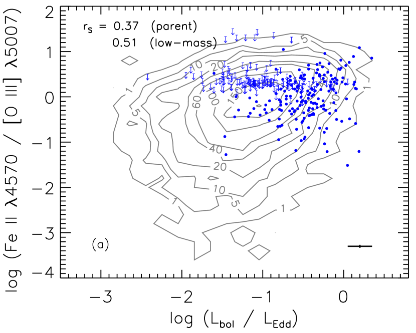
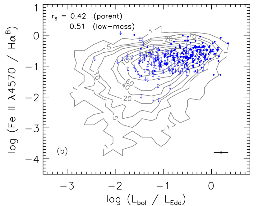
Figure 8: Correlations of the Eddington ratio with the line ratios, Fe II $\lambda 4570$/[O III] $\lambda 5007$ (panel a) and Fe II $\lambda 4570$/(broad H$\alpha$) (panel b), respectively. The contours are for the entire parent broad-line AGN sample and the blue dots are for the present low-mass AGN sample. Also denoted are the Spearman correlation coefficient $r_{\rm\scriptscriptstyle S}$ for the two samples. The symbols are the same as in Figure 3.

With accurate flux measurements of the broad H$\alpha$, Fe II $\lambda 4570$, and [O III] $\lambda 5007$ emission lines, it would be interesting to explore for the first time the emission-line properties of low-mass AGNs in the framework of the eigenvector 1 AGN parameter space of Boroson & Green (1992; EV1 or PC1). EV1 is dominated by the anticorrelation between the strengths of Fe II $\lambda 4570$ and [O III] $\lambda 5007$, and is suggested to be physically driven by the relative accretion rate or the Eddington ratio (Boroson & Green 1992; Marziani et al. 2001; Boroson 2002; cf. Dong et al. 2011; Zhang et al. 2011). In a detailed re-analysis of this issue using a large, homogenous AGN sample, Dong et al. (2011) found that the intensity ratio of Fe II $\lambda 4570$ to [O III] $\lambda 5007$ indeed correlates most strongly with $L\mathrm{{}_{bol}}/L\mathrm{{}_{Edd}}$, whereas the apparent correlations with broad-line width, luminosity, and $M_{\mathrm{BH}}$ are only a secondary effect. Surprisingly, however, Dong et al. (2011) also found that the correlation of Fe II/[O III] with $L\mathrm{{}_{bol}}/L\mathrm{{}_{Edd}}$ is not as strong as that of the EW of Fe II $\lambda 4570$ itself, and actually much weaker than that of the intensity ratio of Fe II $\lambda 4570$ to other broad lines (such as broad H$\beta$ and Mg II $\lambda 2800$). We carry out similar analysis for our low-mass AGN sample. Here we use broad H$\alpha$ instead of broad H$\beta$, and adopt the generalized Spearman rank correlation test to account for censored data. It turns out that the correlations of both Fe II/[O III] and Fe II/H$\alpha^{\rm B}$ with $L\mathrm{{}_{bol}}/L\mathrm{{}_{Edd}}$ are much stronger than those with FWHM(H$\alpha$^B), H$\alpha$^B luminosity, or $M_{\mathrm{BH}}$; this is just as expected, given the restricted ranges of the latter three quantities for the low-mass AGN sample. Moreover, both intensity ratios have equally strong correlations with $L\mathrm{{}_{bol}}/L\mathrm{{}_{Edd}}$, with Spearman coefficients $r_{\rm\scriptscriptstyle S}=0.51$ (a chance probability $P_{\mathrm{null}}=7\times 10^{-27}$). The same analysis is also performed using the parent sample, taking advantage of its large dynamic ranges in both $L\mathrm{{}_{bol}}/L\mathrm{{}_{Edd}}$ and $M_{\mathrm{BH}}$ (Figure 3). Again, both intensity ratios have the strongest correlations with $L\mathrm{{}_{bol}}/L\mathrm{{}_{Edd}}$, and the one involving Fe II/H$\alpha^{\rm B}$ has a slightly higher correlation coefficient ($r_{\rm\scriptscriptstyle S}=0.42$ vs. 0.37). The correlations with $L\mathrm{{}_{bol}}/L\mathrm{{}_{Edd}}$ are illustrated in Figure 8.

Note that, since $M_{\mathrm{BH}}\propto{\rm FWHM}^{2}$, most of the low-mass AGNs in the sample would be classified as narrow-line Seyfert 1s (NLS1s) based on their modest values of H$\alpha$ FWHM. In fact, some of the objects are included in the SDSS NLS1 sample of Zhou et al. (2006). NLS1s are observationally defined as Seyfert 1s having broad H$\beta$ FWHM $\lesssim 2000$ $\mathrm{km~{}s^{-1}}$, often characterized by strong Fe II/H$\beta$ and weak [O III]/H$\beta$ in their optical spectra (see, e.g., Laor 2000 and Komossa 2008 for reviews). Their narrower broad lines are generally believed to arise from their smaller BH masses compared to normal Seyfert nuclei, and their multi-wavelength properties are found to lie at the extreme end of EV1 associated with high accretion rates (Boroson & Green 1992; cf. Desroches et al. 2009 for a recent discussion). Given that in this sample we have made efforts to find low-mass BHs at low accretion rates, most of the objects do not accrete close to the Eddington limit; the median $L\mathrm{{}_{bol}}/L\mathrm{{}_{Edd}}$ is only 0.2 (see Figures 3 and 4 and Table 4). We refer readers to Greene & Ho (2007b; their Section 3.2) and Ai et al. (2011; their Section 6.3) for more detailed discussions on low-mass AGNs and their relationship to NLS1s.

4.2 Properties of the Host Galaxies

Since the discovery of massive BHs at the centers of galaxies, there have been several long-standing puzzles. Is there a lower limit to the mass of central BHs? What are the smallest galaxies harboring central BHs? What is the connection between the BH and the host galaxy in the low-mass regime? Studies on the present sample may contribute to the understanding of these questions. Below we present some preliminary results on the host galaxy properties based on the SDSS imaging data.

4.2.1 Luminosities

We calculate the host galaxy luminosities in the same way as Greene & Ho (2007b). The contribution of the AGN light to the total Petrosian $g$-band magnitude is subtracted by using the H$\alpha$ luminosity to predict the contribution of the AGN continuum to the broad-band photometric magnitude. This is accomplished using the $L_{\rm H\alpha}$–$L_{5100}$ relation of Greene & Ho (2005b) and assuming that the AGN continuum follows the shape $f_{\lambda}\propto\lambda^{-1.56}$ (Vanden Berk et al. 2001). Because of the possibility of aperture losses, we do not trust host galaxy estimates based on the starlight decomposition of the spectra. $K$-corrections of the host galaxy magnitudes are estimated using the routine of Blanton & Roweis (2007). The distributions of the AGN, host, and total luminosities are displayed in Figure 9 (black); also plotted are the corresponding distributions from Greene & Ho (2007b), both their uniformly selected sample (red, solid) and their entire sample (red, dotted). Compared to the Greene & Ho (2007b) sample, while the present sample has more objects with low AGN luminosities, it contains, interestingly, more objects with higher host galaxy luminosities. This presumably reflects the fact that we have put special effort to detect sources with weaker emission lines, as a consequence of which we can tolerate objects with a more significant host galaxy starlight contribution. The present sample has a median AGN luminosity of $M_{g}=-17.7$ mag and a median host galaxy luminosity of $M_{g}=-20.2$ mag, 0.7 mag fainter and 0.9 mag brighter, respectively, than the corresponding medians of the uniformly selected sample of Greene & Ho (2007b). Almost all the host galaxies (304 of 309) are brighter than their nuclei; their luminosity differences have a median of 2.5 mag and a standard deviation of 1.2 mag. The peak of the host galaxy luminosity distribution is comparable to the characteristic luminosity of $M_{g}^{*}=-20.1$ mag at $z=0.1$ (for our assumed cosmology; Blanton et al. 2003), and only 10 objects have host galaxy luminosities $M_{g}>-18.0$ mag. Note that our method of AGN–host separation tends to underestimate the AGN luminosity because of fiber losses, and hence the host galaxy luminosity is generally overestimated. According to the experiments of Greene & Ho (2007b), typically the systematic overestimation should be within 0.3 mag. Another source of error comes from the conversion from H$\alpha$ luminosity to $g$-band magnitude and the assumed continuum slope; it is estimated to be $\sim 0.1$ mag (1 $\sigma$).

4.2.2 Colors and Morphologies

Due to the short exposure time (54 seconds) and mediocre seeing conditions ($\sim$1$\farcs$5) of the SDSS images, direct visual classification of galaxy morphology is impossible for most of the objects in this sample, even those at $z<0.05$. Although the AGN contribution is not large in many cases, the central point source nonetheless significantly affects the central structure of the host. Disk features such as spiral arms and rings are generally smeared out, making it hard to distinguish face-on disks from elliptical or spheroidal galaxies without images of much higher resolution (Greene et al. 2008; Jiang et al. 2011). Following Greene & Ho (2007b), we try to ascertain some rough information from galaxy colors, with the AGN contribution removed from the Petrosian magnitudes. The $u-g$ colors have a mean value of 1.15 mag with a standard deviation of 0.35 mag; the $g-r$ colors have a mean of 0.57 mag and a standard deviation of 0.13 mag. According to Fukugita et al. (1995), these colors correspond to typical values of Sbc galaxies.

4.2.3 Stellar Populations

We briefly examine the stellar populations of the host galaxies of our low-mass BHs using two stellar indexes, the 4000 Å break ($D_{4000}$) and the rest-frame equivalent width of the H$\delta$ absorption line (H$\delta_{\rm A}$). As discussed in Kauffmann et al. (2003a), $D_{4000}$ is an excellent age indicator for young stellar populations ($D_{4000}<1.5$ for ages $<1$ Gyr), while for older populations it also depends strongly on metallicity. H$\delta_{\rm A}$ also does not depend strongly on metallicity except for old populations. Large H$\delta_{\rm A}$ values indicate a burst of star formation that ended 0.1–1 Gyr ago. Altogether, the locus of galaxies in the $D_{4000}$–H$\delta_{\rm A}$ plane is a powerful diagnostic of whether stars have been forming continuously or in bursts over the past 1–2 Gyr. Galaxies with continuous star formation histories occupy an intrinsically very narrow strip in the plane (without taking into account measurement errors of the indices), whereas recent starbursts have large H$\delta_{\rm A}$ values, significantly displaced away from the locus of continuous star formation histories (Kauffmann et al. 2003a).

We take Kauffmann et al.’s (2003a) definition and calculation method of the two indices. The calculation is based on the spectrum of the decomposed starlight component, as described in Section 2.2. For reliable measurement of the indices, we only use the 262 objects that have AGN contribution less than 75% at 4000 Å in the SDSS spectra (cf. Zhou et al. 2006). For comparison, we also calculate the two indexes for $\sim$318,500 inactive galaxies in the SDSS DR4 that have S/N $>5$ pixel^-1 around 4000 Å. For normal galaxies the typical 1 $\sigma$ errors on $D_{4000}$ are 0.05, but for H$\delta_{\rm A}$ they are substantial, on the order of 1.4 Å (Kauffmann et al. 2003b). For our low-mass AGN hosts, the measurement errors should be even larger due to the additional uncertainty from the AGN-host decomposition. We assign an uncertainty of 15% to the decomposition (Zhou et al. 2006) and estimate total 1 $\sigma$ errors on $D_{4000}$ and H$\delta_{\rm A}$ to be 0.1 and 1.6 Å, respectively.

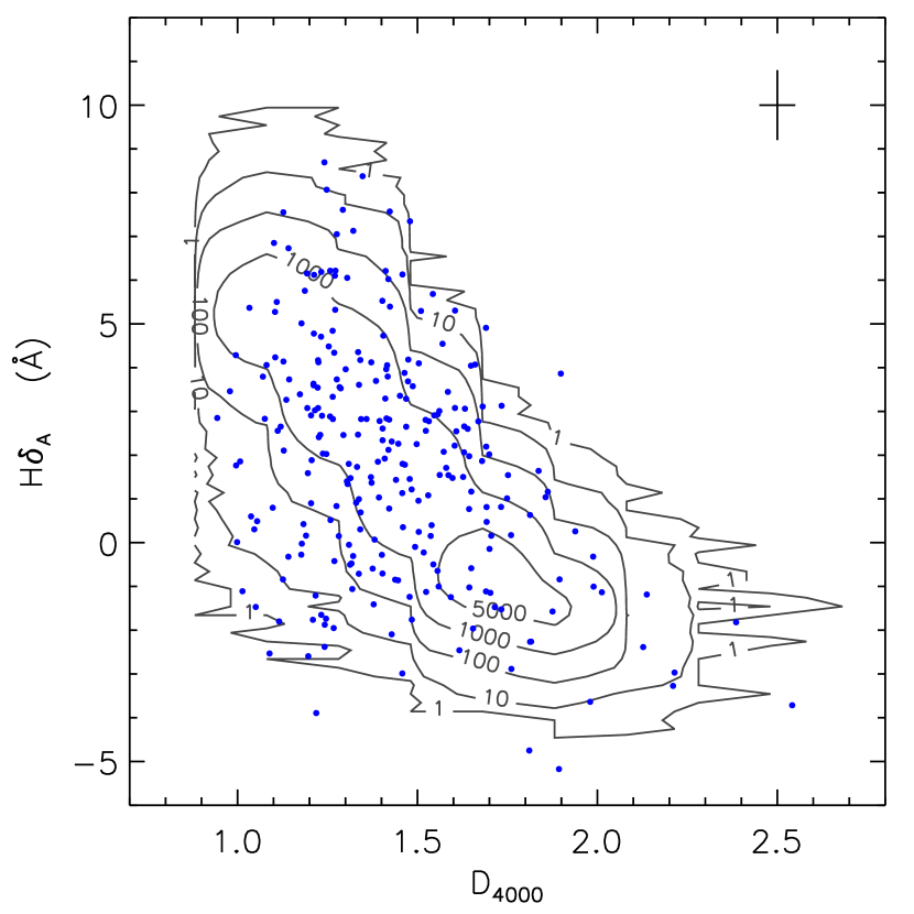
Figure 10: Distribution of the 262 low-mass BH host galaxies (blue dots) in the plane of two stellar indexes, the 4000 Å break and the equivalent width of the H$\delta$ absorption. These objects have an AGN contribution less than 75% at 4000 Å in their SDSS spectra. For comparison the distribution of 318,500 inactive galaxies in the SDSS DR4 is also plotted in contours. The symbols are the same as in Figure 3.

Figure 10 shows the distribution of the 262 low-mass AGN hosts in the $D_{4000}$–H$\delta_{\rm A}$ plane, superposed on contours for the SDSS inactive galaxies. Note that the negative values of H$\delta_{\rm A}$ are not caused by contamination from H$\delta$ emission, but due to the definition and corresponding calculation method of the line index (see Kauffmann et al. 2003a; Worthey & Ottaviani 1997). A few results can be inferred. First, the majority of the low-mass AGN hosts (174 out of 262) have $D_{4000}<1.5$—that is, they have mean stellar ages less than 1 Gyr. Second, although the measurement errors are large, the distribution of the low-mass BH hosts generally overlaps with the locus of continuous star formation histories, in broad agreement with the situation for most inactive galaxies (cf. Figure 3 of Kauffmann et al. 2003a). This finding is consistent with the idea that the evolution of the host galaxies of low-mass BHs is governed principally by secular evolution (Greene et al. 2008; Jiang et al. 2011).

5 Summary

Large-scale optical spectroscopic surveys remain the most effective way to carry out a direct census of active massive BHs over a broad range of masses and accretion rates. We have developed an effective automated selection procedure to select broad-line AGNs from the SDSS spectral archive, with special emphasis on building a uniform sample of AGNs with low BH masses that is more complete toward the faint end of the luminosity function. Particular care is given to AGN-galaxy spectral decomposition and emission-line deblending. Applying our methodology to the SDSS DR4, we compile a new sample of 309 broad-line AGNs with $M_{\mathrm{BH}}<2\times 10^{6}$ $M_{\odot}$, drawn from a parent sample of 8862 sources at $z<0.35$. The BH masses are estimated from the luminosity and the width of the broad H$\alpha$ line, using the virial mass formalism of Greene & Ho (2005b, 2007b). In detail, significant differences exist between the sample of low-mass AGNs compiled here and that published by Greene & Ho (2007b); many are discovered for the first time. The BH masses span the range $8\times 10^{4}-2\times 10^{6}$ $M_{\odot}$, with a median of $1.2\times 10^{6}$ $M_{\odot}$. The broad H$\alpha$ luminosities range from $10^{38.5}$ to $10^{42.3}$ erg s^-1, and FWHMs from 490 to 2380 $\mathrm{km~{}s^{-1}}$ (corrected for instrumental broadening). The Eddington ratios range from $\lesssim 0.01$ to $\sim 1$, and 89 (30%) objects have $L\mathrm{{}_{bol}}/L\mathrm{{}_{Edd}}\leqslant 0.1$. Compared to the previous, most comprehensive catalog of low-mass AGNs (Greene & Ho 2007b), our sample contains more systems accreting at a low Eddington rate ($L\mathrm{{}_{bol}}/L\mathrm{{}_{Edd}}<0.1$).

We present some initial statistical results of this new low-mass AGN sample, focusing on basic properties of the emission lines and host galaxies that can be easily ascertained from the SDSS database. The host galaxies have $g$-band luminosities from $-22.2$ to $-15.9$ mag, with a median value comparable to $L^{*}$, and have $u-g$ and $g-r$ colors typical of Sbc galaxies. We analyze $D_{4000}$ and H$\delta_{\rm A}$, two stellar indices sensitive to age, and conclude that the majority of the host galaxies (174 out of 262) have mean stellar ages less than 1 Gyr. In general the hosts of low-mass AGNs have experienced a history of continuous star formation, consistent with the proposition, based on detailed analysis of their morphologies (Jiang et al. 2011), that these galaxies evolve mainly through secular processes.

Considering the selection effects that seriously act against finding low-mass BHs at low accreting rates, our result implies that a significant number of such low-mass BHs likely exist at the centers of galaxies in the local Universe. This is also supported by the detections of low-luminosity AGNs in very late-type disk galaxies in the X-ray or infrared bands (see, e.g., Desroches & Ho 2009). One interesting question is whether there exists a lower limit to the mass of massive black holes at the centers of galaxies. Our result indicates that, if indeed there is any, this limit should be below a few times $10^{5}$ $M_{\odot}$ at least. Future deeper optical spectroscopic surveys, such as the bigBOSS project, may shed new light on the answer of this question by pushing the BH mass limit even lower.

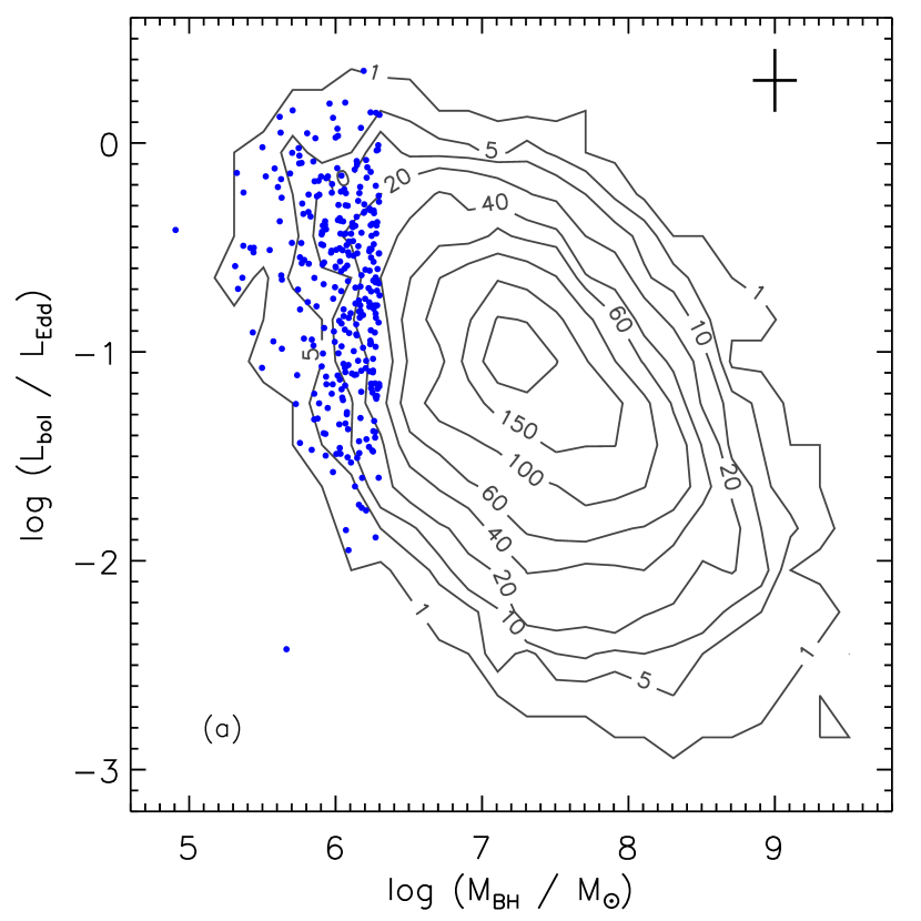
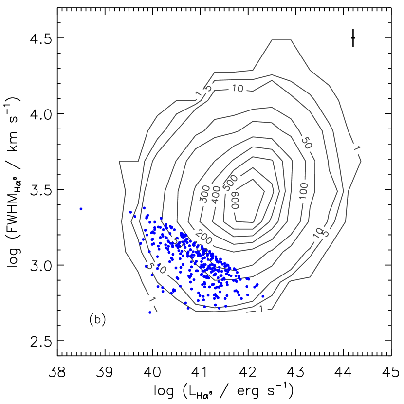
Figure 3: Distribution of our low-mass BH sample (blue dots) in the $L\mathrm{{}_{bol}}/L\mathrm{{}_{Edd}}$ vs. $M_{\mathrm{BH}}$ plane (panel a) and the FWHM vs. luminosity plane for the broad H$\alpha$ line (panel b), respectively. Over-plotted are the contours of the parent 8862 broad-line AGNs at $z<0.35$ uniformly selected from the SDSS DR4. The top-right corner of each panel shows a representative error bar, the length of which corresponds to the 1 $\sigma$ total error (see Section 2.3).

Figure 4: Comparison of the $L\mathrm{{}_{bol}}/L\mathrm{{}_{Edd}}$ distribution of our low-mass BH sample with that of Greene & Ho (2007b).

Figure 7: Narrow-line diagnostic diagrams of [O III] $\lambda 5007$/H$\beta$ vs. [N II] $\lambda 6583$/H$\alpha$ (a), vs. [S II] $\lambda\lambda 6716,6731$/H$\alpha$ (b), and vs. [O I] $\lambda 6300$/H$\alpha$ (c) for our low-mass BH AGN sample. The dotted, curved lines separating H II regions, AGNs and LINERs are taken from Kewley et al. (2001) and Kewley et al. (2006), respectively. In panel (a), the dashed line is an empirical demarcation between H II regions and AGNs given by Kauffmann et al. (2003), and the dotted horizontal line corresponds to [O III] $\lambda 5007$/H$\beta$ $=3$, a traditional line separating AGN and LINERs. The symbols are the same as in Figure 3.

Figure 9: Distributions of the absolute magnitudes in the $g$-band pertaining to the AGN only (top), the host galaxy (middle), and the total (AGN and host galaxy) (bottom), for this sample (black solid line), the uniformly selected sample of Greene & Ho (2007) (green solid lines) and their entire sample (green dotted line). The AGN contribution is estimated from the broad H$\alpha$ luminosity using the $L_{\rm H\alpha}$–$L_{5100}$ relation of Greene & Ho (2005[b]) and assuming a power-law continuum slope $\beta=-1.56$ ($f_{\lambda}\propto\lambda^{\beta}$; Vanden Berk et al. 2001).

Table 1: The SDSS Sample

ID	SDSS Name	$z$	$g$	$g-r$	$A_{g}$
(1)	(2)	(3)	(4)	(5)	(6)
1	J000111.15$-$100155.7	0.0489	18.65	0.78	0.15
2	J000308.48$+$154842.2	0.1175	18.31	0.55	0.14
3	J001728.84$-$001826.8	0.1118	17.85	0.74	0.10

Note. — Col. (1): Identification number assigned in this paper. Col. (2): Official SDSS name in J2000.0. Col. (3): Redshift measured by the SDSS pipeline. Col. (4): Petrosian $g$ magnitude, uncorrected for Galactic extinction. Col. (5): Petrosian $g-r$ color. Col. (6): Galactic extinction in the $g$ band. (This table is available in its entirety in a machine-readable form in the online journal. A portion is shown here for guidance regarding its form and content.)

Table 2: Emission-line Measurements

ID	[O II] $\lambda 3727$	Fe II $\lambda 4570$	H$\beta^{\rm N}$	H$\beta^{\rm B}$	[O III] $\lambda 5007$	[O I] $\lambda 6300$	H$\alpha^{\rm N}$	H$\alpha^{\rm B}$	[N II] $\lambda 6583$	[S II] $\lambda 6716$	[S II] $\lambda 6731$	FWHM${}_{\rm H\alpha^{B}}$	FWHM${}_{\rm[O\,III]}$	FWHM${}_{\rm[S\,II]}$
(1)	(2)	(3)	(4)	(5)	(6)	(7)	(8)	(9)	(10)	(11)	(12)	(13)	(14)	(15)
1	$-$15.12	$<-$15.45	$-$15.39	$<-$15.76	$-$14.79	$-$15.84	$-$14.65	$-$14.71	$-$15.08	$-$15.28	$-$15.46	1921	215	195
2	$-$15.32	$-$15.19	$-$15.61	$-$15.34	$-$15.44	$-$16.11	$-$15.08	$-$14.78	$-$15.51	$-$15.74	$-$15.87	924	164	158
3	$-$15.34	$<-$15.38	$-$15.40	$<-$15.81	$-$15.13	$-$16.12	$-$14.74	$-$14.62	$-$14.95	$-$15.49	$-$15.53	1022	168	256

Note. — Col. (1): Identification number assigned in this paper. Cols. (2)–(12): Emission-line fluxes (or 3 $\sigma$ upper limits) in log-scale, in units of $\mathrm{erg~{}s^{-1}~{}cm^{-2}}$. Note that these are observed values; no NLR or BLR extinction correction has been applied. The superscripts “N” and “B” in cols. 4, 5, 8, 9 and 13 refer to the narrow and broad components of the line, respectively. Cols. (13)–(15): Line widths (FWHM) that are calculated from the best-fit models and have been corrected for instrumental broadening using the values measured from arc spectra and tabulated by the SDSS; in units of $\mathrm{km~{}s^{-1}}$. (This table is available in its entirety in a machine-readable form in the online journal. A portion is shown here for guidance regarding its form and content.)

Table 3: Luminosity and Mass Measurements

ID	$M_{g}$(total)	$M_{g}$(AGN)	$M_{g}$(host)	log $L_{\rm H\alpha^{B}}$	log $M_{\rm BH}$	log $L_{\rm bol}/L_{\rm Edd}$
(1)	(2)	(3)	(4)	(5)	(6)	(7)
1	$-$18.30	$-$15.65	$-$18.20	40.04	6.2	$-$1.6
2	$-$20.66	$-$17.23	$-$20.61	40.77	5.9	$-$0.6
3	$-$21.06	$-$17.47	$-$21.02	40.89	6.0	$-$0.7

Note. — Col. (1): Identification number assigned in this paper. Col. (2): Total $g$-band absolute magnitude. Col. (3): AGN $g$-band absolute magnitude, estimated from $L_{\rm H\alpha^{B}}$ given in col. (5) and a conversion from $L_{\rm H\alpha}$ to $M_{g}$ assuming $f_{\lambda}\propto\lambda^{-1.56}$. Col. (4): Host galaxy $g$-band absolute magnitude, obtained by subtracting the AGN luminosity from the total luminosity. Col. (5): Luminosity of broad H$\alpha$, in units of erg s^-1. Col. (6): Virial mass estimate of the BH, in units of $M_{\odot}$. Col. (7): Eddington ratio. (This table is available in its entirety in a machine-readable form in the online journal. A portion is shown here for guidance regarding its form and content.)

Table 4: Comparison with the low-mass BH sample of Greene & Ho (2007b)

Sample	$N$	log $z$	log $L_{\rm H\alpha^{B}}$	log FWHM${}_{\rm H\alpha^{B}}$	log $M_{\mathrm{BH}}$	log $L\mathrm{{}_{bol}}/L\mathrm{{}_{Edd}}$
GH07b entire sample	229	$-1.06$; 0.25	41.1; 0.6	3.0; 0.1	6.1; 0.2	$-0.5$; 0.5
GH07b uniformly selected sample	174	$-1.01$; 0.23	41.3; 0.4	3.0; 0.1	6.1; 0.2	$-$0.4; 0.3
our uniformly selected sample	309	$-1.03$; 0.25	41.0; 0.6	3.0; 0.1	6.1; 0.2	$-$0.7; 0.5
our newly found subset	61	$-1.06$; 0.27	40.5; 0.6	3.1; 0.2	6.1; 0.2	$-$1.1; 0.5

References

- Adelman-McCarthy et al. (2006) Adelman-McCarthy, J. K., et al. 2006, ApJS, 162, 38
- Ai et al. (2011) Ai, Y. L., Yuan, W., Zhou, H. Y., Wang, T. G., & Zhang, S. H. 2011, ApJ, 727, 31
- Baldwin et al. (1981) Baldwin, J. A., Phillips, M. M., & Terlevich, R. 1981, PASP, 93, 5
- Barth et al. (2008) Barth, A. J., Greene, J. E., & Ho, L. C. 2008, AJ, 136, 1179
- Barth et al. (2004) Barth, A. J., Ho, L. C., Rutledge, R. E., & Sargent, W. L. W. 2004, ApJ, 607, 90
- Becker, White, & Helfand (1995) Becker, R. H., White, R. L., & Helfand, D. J. 1995, ApJ, 450, 559
- Bentz et al. (2009) Bentz, M. C., Peterson, B. M., Netzer, H., Pogge, R. W., & Vestergaard, M. 2009, ApJ, 697, 160
- Bentz et al. (2006) Bentz, M. C., Peterson, B. M., Pogge, R. W., Vestergaard, M., & Onken, C. A. 2006, ApJ, 644, 133
- Blanton & Roweis (2007) Blanton, M. R., & Roweis, S. 2007, AJ, 133, 734
- Blanton (2003) Blanton, M. R., et al. 2003, ApJ, 592, 819
- Boroson (2002) Boroson, T. A. 2002, ApJ, 565, 78
- Boroson & Green (1992) Boroson, T. A. & Green, R. F. 1992, ApJS, 80, 109
- Bruzual & Charlot (2003) Bruzual, G., & Charlot, S. 2003, MNRAS, 344, 1000
- Collin et al. (2006) Collin, S., Kawaguchi, T., Peterson, B. M., & Vestergaard, M. 2006, A&A, 456, 75
- Desroches et al. (2009) Desroches, L.-B., Greene, J. E., & Ho, L. C. 2009, ApJ, 698, 1515
- Desroches & Ho (2009) Desroches, L.-B., & Ho, L. C. 2009, ApJ, 690, 267
- Dong et al. (2010) Dong, X.-B., Ho, L. C., Wang, J.-G., Wang, T.-G., Wang, H., Fan, X., & Zhou, H. 2010, ApJ, 721, L143
- Dong et al. (2011) Dong, X.-B., Wang, J.-G., Ho, L. C., Wang, T.-G., Fan, X., Wang, H., Zhou, H., & Yuan, W. 2011, ApJ, 736, 86
- Dong et al. (2008) Dong, X., Wang, T., Wang, J., Yuan, W., Zhou, H., Dai, H., & Zhang, K. 2008, MNRAS, 383, 581
- Dong et al. (2007) Dong, X., Wang, T., Yuan, W., Zhou, H., Shan, H., Wang, H., Lu, H., & Zhang, K. 2007b, in The Central Engine of Active Galactic Nuclei, ed. L. C. Ho & J.-M. Wang (San Francisco,: ASP), 57
- Dong et al. (2005) Dong, X.-B., Zhou, H.-Y., Wang, T.-G., Wang, J.-X., Li, C., & Zhou, Y.-Y. 2005, ApJ, 620, 629
- Dong et al. (2007) Dong, X., et al. 2007a, ApJ, 657, 700
- Elvis et al. (1994) Elvis, M., et al. 1994, ApJS, 95, 1
- Ferrarese & Merritt (2000) Ferrarese, L., & Merritt, D. 2000, ApJ, 539, L9
- Filippenko & Ho (2003) Filippenko, A. V., & Ho, L. C. 2003, ApJ, 588, L13
- Filippenko, Ho, & Sargent (1993) Filippenko, A. V., Ho, L. C., & Sargent, W. L. W. 1993, ApJ, 410, L75
- Fitzpatrick (1999) Fitzpatrick, E. L. 1999, PASP, 111, 63
- Gebhardt et al. (2000) Gebhardt, K., et al. 2000, ApJ, 539, L13
- Greene& Ho (2004) Greene, J. E., & Ho, L. C. 2004, ApJ, 610, 722
- Greene & Ho (2005a) Greene, J. E., & Ho, L. C. 2005a, ApJ, 627, 721
- Greene & Ho (2005b) Greene, J. E., & Ho, L. C. 2005b, ApJ, 630, 122
- Greene & Ho (2007) Greene, J. E., & Ho, L. C. 2007a, ApJ, 667, 131
- Greene & Ho (2007) Greene, J. E., & Ho, L. C. 2007b, ApJ, 670, 92
- Haehnelt et al. (1998) Haehnelt, M. G., Natarajan, P., & Rees, M. J. 1998, MNRAS, 300, 817
- Hao et al. (2005) Hao, L., et al. 2005, AJ, 129, 1783
- Heckman (1980) Heckman, T. M. 1980, A&A, 87, 152
- Heckman et al. (2004) Heckman, T. M., Kauffmann, G., Brinchmann, J., Charlot, S., Tremonti, C., & White, S. D. M. 2004, ApJ, 613, 109
- Ho (2004) Ho, L. C. 2004, in Carnegie Observatories Astrophysics Series, Vol. 1: Coevolution of Black Holes and Galaxies, ed. L. C. Ho (Cambridge: Cambridge Univ. Press), 292
- Ho (2008) Ho, L. C. 2008, ARA&A, 46, 475
- Ho (2009) Ho, L. C. 2009, ApJ, 699, 626
- Ho et al. (1997) Ho, L. C., Filippenko, A. V., & Sargent, W. L. W. 1997a, ApJS, 112, 315
- Ho et al. (1997) Ho, L. C., Filippenko, A. V., Sargent, W. L. W., & Peng, C. Y. 1997b, ApJS, 112, 391
- Jiang et al. (2011) Jiang, Y.-F., Greene, J. E., Ho, L. C., Xiao, T., & Barth, A. J. 2011, ApJ in press (arXiv:1107.4105)
- Kaspi et al. (2005) Kaspi, S., Maoz, D., Netzer, H., Peterson, B. M., Vestergaard, M., & Jannuzi, B. T. 2005, ApJ, 629, 61
- Kaspi et al. (2000) Kaspi, S., Smith, P. S., Netzer, H., Maoz, D., Jannuzi, B. T., & Giveon, U. 2000, ApJ, 533, 631
- Kauffmann et al. (2003) Kauffmann, G., et al. 2003a, MNRAS, 341, 33
- Kauffmann et al. (2003) Kauffmann, G., et al. 2003b, MNRAS, 346, 1055
- Kewley et al. (2001) Kewley, L. J., Dopita, M. A., Sutherland, R. S., Heisler, C. A., & Trevena, J. 2001, ApJ, 556, 121
- Kewley et al. (2006) Kewley, L. J., Groves, B., Kauffmann, G., & Heckman, T. 2006, MNRAS, 372, 961 al. 2006, ApJ, 648, 128
- Komossa (2008) Komossa, S. 2008, Revista Mexicana de Astronomia y Astrofisica Conference Series, 32, 86
- Kormendy & Kennicutt (2004) Kormendy, J., & Kennicutt, R. C., Jr. 2004, ARA&A, 42, 603
- Laor (2000) Laor, A. 2000, New Astronomy Reviews, 44, 503
- Laor (2007) Laor, A. 2007, in The Central Engine of Active Galactic Nuclei, ed. L. C. Ho & J.-M. Wang (San Francisco: ASP), 384
- Lu et al. (2006) Lu, H., Zhou, H., Wang, J., Wang, T., Dong, X., Zhuang, Z., & Li, C. 2006, AJ, 131, 790
- Lu et al. (2010) Lu, Y., Wang, T.-G., Dong, X.-B., & Zhou, H.-Y. 2010, MNRAS, 404, 1761
- Magorrian et al. (1998) Magorrian, J., et al. 1998, AJ, 115, 2285
- Markwardt (2009) Markwardt, C. B. 2009, in Astronomical Data Analysis Software and Systems XVIII, ed. D. A. Bohlender, D. Durand, & P. Dowler (San Francisco: ASP), 251
- Marziani et al. (2001) Marziani, P., Sulentic, J. W., Zwitter, T., Dultzin-Hacyan, D., & Calvani, M. 2001, ApJ, 558, 553
- McLure & Dunlop (2004) McLure, R. J., & Dunlop, J. S. 2004, MNRAS, 352, 1390
- Moran et al. (1999) Moran, E. C., Filippenko, A. V., Ho, L. C., Shields, J. C., Belloni, T., Comastri, A., Snowden, S. L., & Sramek, R. A. 1999, PASP, 111, 801
- Peterson & Wandel (1999) Peterson, B. M., & Wandel, A. 1999, ApJ, 521, L95
- Peterson & Wandel (2000) Peterson, B. M., & Wandel, A. 2000, ApJ, 540, L13
- Peterson et al. (2005) Peterson, B. M., et al. 2005, ApJ, 632, 799
- Richards et al. (2002) Richards, G. T., et al. 2002, AJ, 123, 2945
- Satyapal et al. (2008) Satyapal, S., Vega, D., Dudik, R. P., Abel, N. P., & Heckman, T. 2008, ApJ, 677, 926
- Schlegel, Finkbeiner, & Davis (1998) Schlegel, D. J., Finkbeiner, D. P., & Davis, M. 1998, ApJ, 500, 525
- Schulze & Wisotzki (2010) Schulze, A., & Wisotzki, L. 2010, A&A, 516, A87
- Stoughton et al. (2002) Stoughton, C. et al. 2002, AJ, 123, 485
- Sulentic et al. (2006) Sulentic, J. W., Repetto, P., Stirpe, G. M., Marziani, P., Dultzin-Hacyan, D., & Calvani, M. 2006, A&A, 456, 929
- Vanden Berk et al. (2001) Vanden Berk, D. E., et al. 2001, AJ, 122, 549
- van der Marel (2004) van der Marel, R. P. 2004, in Carnegie Observatories Astrophysics Series, Vol. 1: Coevolution of Black Holes and Galaxies, ed. L. C. Ho (Cambridge: Cambridge Univ. Press), 37
- Veilleux & Osterbrock (1987) Veilleux, S., & Osterbrock, D. E. 1987, ApJS, 63, 295
- Verolme et al. (2002) Verolme, E. K., et al. 2002, MNRAS, 335, 517
- Véron-Cetty et al. (2004) Véron-Cetty, M.-P., Joly, M., & Véron, P. 2004, A&A, 417, 515
- Vestergaard & Peterson (2006) Vestergaard, M., & Peterson, B. M. 2006, ApJ, 641, 689
- Voges et al. (1999) Voges, W., et al. 1999, A&A, 349, 389
- Volonteri et al. (2008) Volonteri, M., Lodato, G., & Natarajan, P. 2008, MNRAS, 383, 1079
- Wang et al. (2009) Wang, J.-G., Dong, X.-B., Wang, T.-G., Ho, L. C., Yuan, W., Wang, H., Zhang, K., Zhang, S., Zhou, H. 2009, ApJ, 707, 1334
- Worthey & Ottaviani (1997) Worthey, G., & Ottaviani, D. L. 1997, ApJS, 111, 377
- Xiao et al. (2011) Xiao, T., Barth, A. J., Greene, J. E., Ho, L. C., Bentz, M. C., Ludwig, R. R., & Jiang, Y. 2011, ApJ in press (arXiv:1106.6232)
- York et al. (2000) York, D. G., et al. 2000, AJ, 120, 1579
- Zhou et al. (2006) Zhou, H., Wang, T., Yuan, W., Lu, H., Dong, X., Wang, J., & Lu, Y. 2006, ApJS, 166, 128
- Zhang et al. (2011) Zhang, K., Dong, X.-B., Wang, T.-G., & Gaskell, C. M. 2011, ApJ in press (arXiv:1105.1094)
- Zhang et al. (2008) Zhang, K., Wang, T., Dong, X., & Lu, H. 2008, ApJ, 685, L109
- Zhang et al. (2009) Zhang, K., Wang, T.-G., Dong, X.-B., Zhou, H.-Y., & Lu, H.-L. 2009, in The Starburst-AGN Connection, ed. W. Wang et al. (San Francisco: ASP), 281