X-Ray emission from SN 2004dj: A Tale of Two Shocks

Abstract

Type IIP (Plateau) Supernovae are the most commonly observed variety of core collapse events. They have been detected in a wide range of wavelengths from radio, through optical to X-rays. The standard picture of a type IIP supernova has the blastwave interacting with the progenitor’s circumstellar matter to produce a hot region bounded by a forward and a reverse shock. This region is thought to be responsible for most of the X-ray and radio emission from these objects. Yet the origin of X-rays from these supernovae is not well understood quantitatively. The relative contributions of particle acceleration and magnetic field amplification in generating the X-ray and radio emission need to be determined. In this work we analyze archival Chandra observations of SN 2004dj, the nearest supernova since SN 1987A, along with published radio and optical information. We determine the pre-explosion mass loss rate, blastwave velocity, electron acceleration and magnetic field amplification efficiencies. We find that a greater fraction of the thermal energy goes into accelerating electrons than into amplifying magnetic fields. We conclude that the X-ray emission arises out of a combination of inverse Compton scattering by non-thermal electrons accelerated in the forward shock and thermal emission from supernova ejecta heated by the reverse shock.

1. Introduction

Core collapse supernovae with hydrogen lines near maximum light and a pronounced plateau in their visible band light curve that remain within $\sim 1$ mag of maximum brightness for an extended period are called type IIP supernovae. The plateau duration is often 60-100 rest-frame days and is followed by an exponential tail powered by radioactive decay at late times. Type IIP supernovae constitute about 67% of all core collapse supernovae in a volume limited sample ($d<30$ Mpc) (Smartt et al. 2009). Their characteristic optical light curves are attributed to the hydrogen envelope of the progenitor remaining largely intact before the core collapse. Several lines of evidence suggest that these stars were red supergiants when they exploded. Type II supernovae (as well as the type Ib/c supernovae) are associated with recent star forming regions of the spiral galaxies (Filippenko 1997) which suggest that their progenitor stars are relatively short lived and therefore explode from massive stars ($M>8M_{\odot}$) which have faster burning of their nuclear fuels at generally higher central temperatures compared to less massive stars. Their plateau brightness and duration combined with their expansion velocities suggest a pre-supernova radius of typically red supergiant dimensions (e.g. $10^{2\sim 3}\;R_{\odot}$). While there are more massive red supergiants in the Local Group of galaxies, no high-mass red supergiant progenitors above $17M_{\odot}$ have been found for IIP supernovae in direct detection efforts in volume-limited search for supernova progenitor stars (Smartt et al. 2009). This red supergiant problem has led to a viewpoint that these more massive stars could have core masses high enough to form black holes and supernovae from them could be too faint to have been detected. At the same time a minimum stellar mass for a SN IIP to arise from is about $8.5\pm 1.0\;M_{\odot}$, consistent with the upper limit to white dwarf progenitor masses. A census of type IIP progenitors and the partial loss of their hydrogen envelopes could potentially be important for neutron star vs black hole formation and their number distribution in the galaxy.

In a type IIP supernova, the expanding ejecta interacts with the slow wind of the red supergiant even though the star retained most of its hydrogen envelope intact. This interaction generates a hot region, bounded by the forward and reverse shocks, which may emit thermal X-rays. These shocks may also accelerate charged particles and synchrotron radiation from relativistic electrons can lead to radio emission that is strong enough to be detected at extragalactic distance scales. The measurable radio and X-ray properties give complementary information about the regions shocked by the forward and reverse shocks and can constrain the physical properties of the interaction region and the progenitor star. Because type IIP supernovae have a plateau phase of high optical luminosity, energetic electrons near the forward shock find a dense photon environment of seed photons which may be Compton boosted to X-ray energies. The resultant Compton cooling can affect the population of the electrons which also emit at radio wavelengths and show suppressed radio fluxes above a characteristic cooling break until the end of the plateau phase where the optical photon density undergoes a rapid decline (Chevalier et al. 2006).

Using SN 2004dj as a prototype of its class we would like to address the questions:

1. What is the origin of X-rays detected by the Chandra from young type IIP supernovae?

2. How fast was the progenitor losing mass via winds in the final phase before explosion?

3. How efficiently does the supernova accelerate cosmic ray electrons in its forward shock?

4. What is the extent of turbulent magnetic field amplification in the post-shock material?

5. Are synchrotron and inverse Compton losses important in explaining the radio lightcurves?

SN 2004dj, discovered by K. Itagaki (see Nakano et al. 2004) on 31.76 July 2004 (UT) in the spiral galaxy NGC 2403, was the closest (Karachentsev et al. 2004) normal type IIP SN (Patat et al. 2004) observed to date. It was discovered $50\pm 21$ days (Zhang et al. 2006) after its progenitor’s core collapse and had a peak magnitude of 11.2 mag in the V-band (Zhang et al. 2006). Analysis of its pre-explosion images indicated that the initial main sequence mass of the progenitor of SN 2004dj was about $15\;M_{\odot}$ (Maíz-Apellániz et al. 2004); see however Wang et al. (2005) where the progenitor had a main-sequence mass of $12M_{\odot}$. SN 2004dj occurred at a position coincident with Sandage star number 96 (hereafter S96, and resolved by HST to be a young star cluster) in NGC 2403. To date, only seven supernovae of type IIP are known X-ray emitters. Only four of them are known radio emitters: Supernovae 1999em, 2002hh, 2004dj and 2004et. X-rays from circumstellar interaction has been studied in detail for type IIP supernovae including SN 1999em (Pooley et al. 2002), and 2004et (Misra et al. 2007). Because of its close range, SN 2004dj was easily detectable in the X-ray and radio. The Chandra X-ray Observatory had targeted it multiple times early after its explosion. The earliest detection was reported by Pooley & Lewin (2004).

The X-ray and radio luminosities are both sensitive to the mass loss rate and the initial mass of the progenitor star. In this paper we demonstrate that for SN 2004dj the determination of the inverse Compton powerlaw spectrum from the forward shock, the characteristics of the X-ray line emitting thermal plasma from the reverse shock and the radio light curve peak, uniquely determines some properties of the explosion and the progenitor star. These include the pre-supernova mass loss rate $(\dot{M})$, the fraction of post-shock energy density which goes into relativistic electrons $(\epsilon_{e})$ magnetic fields $(\epsilon_{B})$. The time dependent nature of the thermal and non-thermal X-ray fluxes also bear signatures of the circumstellar density profile as the forward shock encounters more and more circumstellar matter and the ejecta profile as the reverse shock ploughs into the expanding ejecta. We also see the correlation of the inverse Compton flux with the optical light curve.

Figure 1.— First X-ray spectrum of SN 2004dj on 2004 August 9. Bars are counts from Chandra, binned for display. Dotted line is the powerlaw model for the inverse Compton flux. Dashed line is the APEC model for the thermal plasma. Solid line is the full model. Note that the full model is dominated by the non-thermal flux even at $\sim 1$ keV.

2. Observations of SN 2004dj

As the nearest ($\sim 3$ Mpc) supernova since SN 1987A, SN 2004dj enjoyed extensive multi-wavelength coverage. The details of the observations in Radio, Optical and X-rays, used in this work, are given below.

2.1. Chandra X-Ray Observations

SN 2004dj was observed by a Target of Opportunity program (PI: Walter Lewin, Cycle: 5, ObsIDs: 4627-4630) using the Chandra X-ray Observatory on four occasions: 2004 August 9 (See Fig 1), August 23, October 3 and December 22 (See Fig 2). The ACIS-S chips were used on all occasions, without any grating, for 50 ks each. The supernova was detected in the first of these observations (Pooley & Lewin 2004). We analyze all four observations in this work for the first time. See Table 1 for details of observations.

Table 1Observation summary of SN 2004dj with Chandra

Date	Exposure	Count Rate	Flux (0.5-8 keV)
(2004)	(ks)	($10^{-3}$ sec-1)	(ergs cm-2 s-1)
Aug 09	40.9	$12.80\pm 0.56$	$8.81\times 10^{-14}$
Aug 23	46.5	$10.03\pm 0.47$	$6.98\times 10^{-14}$
Oct 03	44.5	$5.60\pm 0.36$	$3.30\times 10^{-14}$
Dec 22	49.8	$3.05\pm 0.25$	$2.02\times 10^{-14}$

Before spectral analysis, the data from separate epochs were processed separately but in a similar fashion, following the prescribed threads from the Chandra Science Center using CIAO 4.4 with CALDB 4.4.8. The level 2 events were filtered in energy to reject all counts below 0.3 keV and above 10 keV. The resulting events were mapped and the supernova easily identified. The source region was marked off and a light curve was generated from the rest of the counts. Flare times were identified in this light curve, as time-ranges where the count rate rose above 3 times the rms. This resulted in a good time interval table which was used to further filter out the events. The spectrum, response and background files were then generated for these good events. In order to obtain the highest available spectral resolution, the data were not binned; unbinned data were analyzed in the next steps.

2.2. Radio Observations

SN 2004dj has been observed extensively in radio bands from Aug 2004 until May 2007 with various telescopes including the Very Large Array (VLA), Giant Metrewave Radio Telescope (GMRT) and Multi-Element Radio Linked Interferometer Network (MERLIN). MERLIN observed SN 2004dj extensively in the 5 GHz band covering the period from 2004 August 5 to December 2. These observations are reported in Beswick et al. (2005). The GMRT observations started on 2004 Aug 12 and continued until 2007 May 22. The observations were made in the 1420, 610, 325 and 235 MHz bands. The first two GMRT observations in 1420 MHz band are reported in Chandra & Ray (2004). The VLA followed SN 2004dj extensively starting from Aug 1, 2004 until May 28, 2007. The observations were made in all VLA bands starting from 1.4 GHz band upto 44 GHz band. The first 8.4 GHz observation was reported by Stockdale et al. (2004). Chevalier et al. (2006) discussed these published radio observations of SN 2004dj to interpret the physical properties of SN 2004dj and its interaction with the circumstellar matter. They established Free Free Absorption to be the radio absorption mechanism based on the published radio observations. A comprehensive paper including all the radio observations and their detailed interpretation is underway (Chandra et al., 2012, under preparation.)

3. A Tale of Two Shocks

Supernova ejecta hits the pre-explosion wind at a velocity much larger than its characteristic sound speed. This creates a strong forward shock moving into the circumstellar matter arising from the mass loss from the progenitor (Chevalier 1982). In case of a type IIP supernova, the material behind this shock is too hot ($\sim 100$ keV) and tenuous to contribute significantly to the X-ray flux in the Chandra bands ($0.3-10$ keV) through its thermal emission. However, the radio emission from type IIP supernovae is said to arise from the non-thermal electrons accelerated in this region (Chevalier et al. 2006). Some optical photons from a supernova may also be inverse Compton scattered off energetic electrons in this region into the X-rays (Sutaria et al. 2003; Björnsson & Fransson 2004). Scattering from a non-thermal population of electrons with a power law index $p$ generates a spectral index of $(p-1)/2$ in the optically thin radio synchrotron. So the inverse Compton spectrum may be modeled as a power law with a photon index of $(p+1)/2$.

In the frame of the ejecta however, the circumstellar matter impinges supersonically on the ejecta. According to McKee (1974) this drives an inward (in mass coordinates) propagating wave which reheats the ejecta, which would have otherwise been adiabatically cooled by its rapid expansion, to around $\sim 1$ keV. A supernova typically ejects more matter at lower velocity. As the reverse shock moves into slower moving ejecta, its heats up more gas which can contribute to the X-ray flux. The plasma in this region can be modeled as a collisionally-ionized diffuse hot gas.

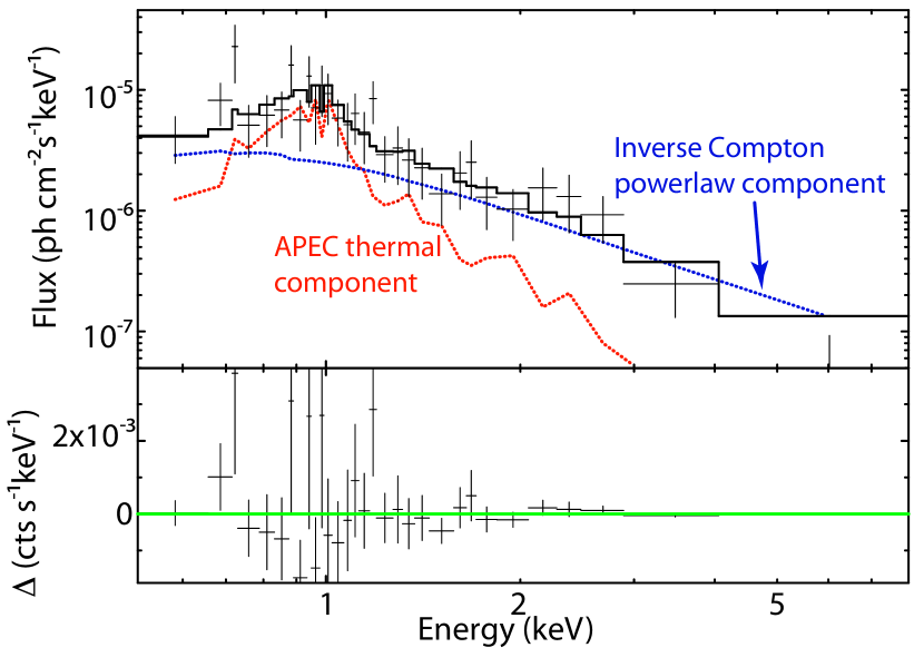
Figure 2.— Last X-ray spectrum of SN 2004dj on 2004 December 22. Note that the relative contribution of the non-thermal inverse Compton, with respect to the flux from the thermal plasma has gone down, when compared with the first epoch. The full model is now dominated by the thermal flux at $\sim 1$ keV.

3.1. X-ray Spectral Fitting

We imported the extracted spectra into XSPEC 12.7.1 for further analysis. The data from all epochs were jointly fitted with the combination of a simple photon power law using powerlaw and collisionally-ionized diffuse gas using APEC models (Smith et al. 2001), passed through a photo-electric absorbing column using wabs. The column density for wabs, plasma temperature for APEC and photon index for powerlaw were shared between all epochs. The emission measure for APEC and normalization for powerlaw were determined separately for each epoch from the joint analysis. As, the fits were performed on unbinned data, each bin would have too few photons for the $\chi^{2}$ statistic to be useful. We therefore used the cstat statistic based on Cash (1979). In order to evaluate the goodness of fit, we simulated 10000 spectra based on the best fit model and found out that only 25% of these simulations had cstat less than that for the data. We therefore conclude that this model provides a good fit to the data. The best fit absorption column density is $n_{\rm H}=(1.7\pm 0.5)\times 10^{21}\;{\rm cm^{-2}}$. See Table 1 for model fluxes on each date.

3.2. Reverse-Shocked Material

A self-similar solution for the interaction of the fast moving ejecta and the nearly static (negligibly moving) circumstellar matter was found by Chevalier (1982). This can be used to generate a complete description of the forward and reverse-shocked material (Nadezhin 1985).

Following Chevalier (1982) we consider supernova ejecta described by

$$\rho_{\rm ej}\propto t^{-3}V^{-\eta},$$ (1)

where the density falls due to free expansion and higher velocities have less matter, described by the power law index $\eta$. This ejecta interacts with the circumstellar matter, described by a power law profile $\rho\propto r^{-s}$. For a steady wind ($s=2$), we have

$$\rho_{\rm w}=\frac{A}{r^{2}}=\frac{\dot{M}}{4\pi r^{2}v_{\rm w}},$$ (2)

where $\dot{M}$ is the mass loss rate and $v_{\rm w}$ is the wind velocity of the progenitor. Here $A=\dot{M}/(4\pi v_{\rm w})$ (Chevalier 1982). Shock jump conditions for a fast shock dictate that the density behind the forward shock is given by $\rho_{\rm cs}=4\rho_{\rm w}$. In the thin shell approximation, this can be further related to the density behind the reverse shock as

$$\rho_{0}=\frac{(\eta-3)(\eta-4)}{(3-s)(4-s)}\rho_{\rm cs}.$$ (3)

According to Matzner & McKee (1999) $\eta$ is expected to be 12 for a red supergiant progenitor. Using this value simplifies the above expression to $\rho_{0}=36\rho_{\rm cs}=144\rho_{\rm w}$.

Therefore the reverse-shocked material is much denser than the circumstellar matter. So it can cool efficiently via radiative processes and contribute to the thermal X-ray flux.

Figure 3.— Confidence contours for Temperature (in the APEC model) vs Photon Index (in the powerlaw model). Note that the Chandra data can successfully break the degeneracy between the two components and account for their most important parameters, namely the temperature and photon index.

3.3. Blastwave Velocity

The velocity of a shock determines the energy imparted to particles crossing it, and hence the post-shock plasma temperatures. Furthermore, the forward and reverse shock velocities are connected by jump conditions once the ejecta and circumstellar matter profile are specified. So, the post-shock temperature of ejecta which has crossed the reverse shock can be expressed in terms of the blastwave velocity. Since the former is an observable, the latter can be derived from it.

Nymark et al. (2006) give the temperature of the reverse-shocked material $T_{0}$, as

$$T_{0}=2.27\times 10^{9}\mu\frac{(3-s)^{2}}{(\eta-s)^{2}}V_{4}^{2}\;\;{\rm K,}$$ (4)

where $\mu$ is the mean atomic weight per particle, $\eta$ is the power law index of the ejecta profile, $s$ is the power law index of the circumstellar density profile and $V_{4}$ is the forward shock velocity in units of $10^{4}$ km s^-1. $\mu$ is 0.61 in the solar-like outermost zone of the progenitor (Nymark et al. 2006). $s$ is 2 for a circumstellar matter set up by a steady wind, and we again use $\eta=12$. With these assumptions, the forward shock velocity can be expressed as

$$V_{s}=10^{4}\;\sqrt{\frac{kT_{0}}{1.19\;{\rm keV}}}\;\;{\rm kms^{-1}}.$$ (5)

Since, the best fit temperature is $0.997\pm 0.054$ keV (See Fig 3), the implied velocity is $V_{s}=(9.2\pm 0.3)\times 10^{3}$ km s^-1.

This is consistent with the fastest-moving ejecta in a typical type IIP supernova. Therefore, the observed thermal component of the X-ray spectrum can be explained as emission from reverse-shocked material, provided this is the blastwave velocity. Chugai et al. (2007) have proposed diagnostics for circumstellar interaction in Type IIP supernovae using the detection of high-velocity absorption features in H$\alpha$ and He I lines during the photospheric stage. The highest velocity H$\alpha$ absorption feature observed in the optical spectra of SN 2004dj is at 8200 km s^-1 between 64 (Chugai et al. 2007) and 102 days (Vinkó et al. 2006) with respect to the explosion date of June 28 proposed by Chugai et al. (2007). This overlaps with the epoch of Chandra observations and provides a lower limit to the allowed forward shock velocity, so the velocity that we obtain is consistent with constraints from optical spectroscopy.

Figure 4.— Confidence contours for normalization of the thermal flux (in the APEC model) the normalization of the non-thermal flux (in the powerlaw model). Note the anti-correlation between the thermal and non thermal fluxes, as their sum must explain the total flux which is fixed by observations.

3.4. Circumstellar Density

The reverse-shocked matter contributes bulk of the thermal X-rays. In order to find the circumstellar density it is necessary to estimate the amount of reverse-shocked material in terms of the forward-shocked material. Using Equations 2 and 3 and again assuming $\eta=12$, we get

$$\rho_{0}=\frac{36\dot{M}}{\pi r^{2}v_{\rm w}}.$$ (6)

Similarly, following Nymark et al. (2006) we can express the total mass of reverse-shocked material as

$$M_{0}=\frac{\eta-4}{4-s}M_{\rm cs}=\frac{4\dot{M}R_{s}}{v_{\rm w}},$$ (7)

where $R_{s}$ is the blastwave radius. Multiplying these two results, we get,

$$\rho_{0}M_{0}=\frac{144}{\pi}\left(\frac{\dot{M}}{v_{\rm w}}\right)^{2}\frac{1}{R_{s}}.$$ (8)

These have to be converted to number densities to get the emission measure which determines the thermal X-ray flux. For a solar-like composition appropriate for the outermost shells of the supernova, $\rho=1.17{\rm amu}\times n_{e}=1.40{\rm amu}\times n_{H}$. Using these, we have the emission measure for the reverse-shocked material as

$$\int n_{e}n_{H}dV=\frac{144}{\pi}\left(\frac{\dot{M}}{v_{\rm w}}\right)^{2}\frac{1}{(1.17{\rm amu})(1.40{\rm amu})R_{s}}$$ (9)

We estimate the shock radius from the velocity determined in the previous Sub-Section as $R_{s}=V_{s}t$, with the time calculated from the explosion date of 2004 June $11\pm 21$ (Zhang et al. 2006) or JD 2,453,168. As all the other quantities are known, the circumstellar density can now be determined from the emission measure.

The APEC fit to the thermal part of the X-ray spectrum of SN 2004dj gives,

$$\frac{10^{-14}}{4\pi[D_{A}(1+z)]^{2}}\int n_{e}n_{H}dv=(7.5\pm 2.7)\times 10^{-6}\;,$$ (10)

for the first epoch (see Fig 4). NGC 2403 is nearby and has negligible redshift. We adopt a distance to NGC 2403 of 3.06 Mpc based on Cepheids from Saha et al. (2006). Eliminating the emission measure between the last two equations, we have,

$$\frac{\dot{M}}{v_{\rm w}}=(2.0\pm 0.7)\times 10^{13}\;{\rm g\;s^{-1}}.$$ (11)

Therefore the mass loss rate of the progenitor was

$$\dot{M}=(3.2\pm 1.1)\times 10^{-7}\left(\frac{v_{\rm w}}{10\;{\rm km/s}}\right)\;{\rm M_{\odot}\;yr^{-1}}$$ (12)

This gives us $A$; however Chevalier & Fransson (2006) define a non-dimensional $A_{\star}=A/(5\times 10^{11}\;{\rm g\;cm^{-1}})$. For SN 2004dj, we therefore get $A_{\star}=3.2\pm 1.1$, which can now be compared with estimates for circumstellar density from the radio emission.

3.5. Forward-Shocked material

Electrons are believed to be accelerated to relativistic velocities in the forward shock. These are in turn, responsible for the radio emission from supernovae. The simplest model by Chevalier (1982), is to assume that a fraction $\epsilon_{e}$ or $\epsilon_{B}$ of the thermal energy is used to accelerate electrons and amplify magnetic fields respectively. As a result the radio emission from a supernova is dependent upon these fractions and does not measure the circumstellar density directly. Instead, according to Chevalier & Fransson (2006), the radio emission measures

$$S_{\star}= A_{\star}\epsilon_{B-1}\alpha^{8/19}=1.0\left(\frac{f}{\texttimes 0.5}\right)^{-8/19}\left(\frac{F_{\rm p}}{\rm mJy}\right)^{-4/19}$$

$$\times\left(\frac{D}{\rm Mpc}\right)^{-8/19}\left(\frac{\nu}{5{\rm\;GHz}}\right)^{-4/19}t_{10}^{2},$$ (13)

where $F_{\rm p}$ is the peak flux at peak frequency $\nu$ at $10\times t_{10}$ days from the explosion and $\epsilon_{B-1}=\epsilon_{B}/0.1$. The equipartition factor is defined as $\alpha\equiv\epsilon_{e}/\epsilon_{B}$. Using the $4.99$ GHz, radio light curve from Beswick et al. (2005) for SN 2004dj, we have $S_{\star}=5.1$.

The same relativistic electrons which generate the radio spectrum via synchrotron emission may also contribute to the X-ray flux by inverse Compton scattering the optical photons from the supernova’s peak bolometric luminosity of around $\sim 10^{42}{\rm\;ergs\;s^{-1}}$. This may explain the dominant non-thermal component seen in the X-ray spectrum at early times (see Fig 1). For an electron index $p=3$ this is expected to generate a powerlaw with photon index 2, consistent with the observations (see Fig 3). Following Chevalier & Fransson (2006) the normalization of the inverse Compton flux at 1 keV can be written as

$$E\frac{dL_{\rm IC}}{dE} \approx 8.8\times 10^{36}\gamma_{\rm min}S_{\star}\alpha^{11/19}V_{4}$$

$$\times\left(\frac{L_{\rm bol}(t)}{10^{42}{\rm\;ergs\;s^{-1}}}\right)t_{10}^{-1}{\rm\;ergs\;s^{-1}},$$ (14)

where $\gamma_{\rm min}$ is the minimum Lorentz factor of the relativistic electrons.

The normalization of the inverse Compton flux obtained for the first epoch ($t_{10}\sim 6$) of Chandra observations, is seen to be $(3.8\pm 0.5)\times 10^{37}{\rm\;ergs\;s^{-1}}$ (see Fig 4). Substituting this in the left hand side and using a $S_{\star}=5.1$ as found in this work, $V_{4}=0.92$ as implied by the temperature of the reverse-shocked plasma, $L_{\rm bol}=0.89\times 10^{42}{\rm\;ergs\;s^{-1}}$ from Zhang et al. (2006), we get

$$\alpha\sim 23\times\gamma_{\rm min}^{-19/11},$$ (15)

where $\gamma_{\rm min}=1$ if the electron spectrum extends all the way down to those at rest. However, if one only considers relativistic electrons with $\gamma_{\rm min}\sim 2.5$ as used by Chevalier & Fransson (2006) for SN 2002ap, it implies $\alpha\sim 4.8$. We prefer this latter (more realistic) assumption as the bulk of the accelerated electrons cannot be at rest or very low velocities. So we shall use this latter value in further calculations.

Now that we know $S_{\star}$ from radio synchrotron, $A_{\star}$ from thermal X-rays and $\alpha$ from inverse Compton, we can use the definition of $S_{\star}$ to get

$$\epsilon_{B}\equiv 0.1\times\epsilon_{B-1}\sim 0.082,$$ (16)

which in turn implies

$$\epsilon_{e}\equiv\alpha\times\epsilon_{B}\sim 0.39\;\;.$$ (17)

Hence we have determined both $\epsilon_{e}$ and $\epsilon_{B}$ using a combination of X-ray, radio and optical data.

Figure 5.— Time evolution of the normalization of the thermal APEC component (proportional to the emission measure) in the spectrum of SN 2004dj obtained from simultaneous fits to Chandra spectra. The time interval is measured with respect to the explosion date of June 11 from Zhang et al. (2006). Line is best fit $\propto t^{-1}$ function. Note that the data do not rule out a constant mass loss rate model, but suggest one with variable mass loss.

4. Time Evolution

The first things that are apparent from the Chandra observations of SN 2004dj is that the total X-ray flux softens and falls with time. These gross features have already been observed in another type IIP supernova, SN 2004et by Rho et al. (2007). However, the quality of the SN 2004dj spectra allows a quantitative explanation for the first time. While both the thermal and non-thermal components fall eventually, their proportion changes with time. At early times, the spectra is dominated by the inverse Compton flux and is therefore harder (see Fig 1). As the bolometric light curve of the supernova decays, the source of seed photons to be scattered turns off. So at late times, the spectra is dominated by emission from the reverse-shocked thermal plasma and is therefore softer (see Fig 2).

4.1. Thermal X-Rays

Since the post shock temperature in a self similar blastwave does not change much, as the shock velocity is slowly varying, the variation in the thermal X-ray flux would come from the variation in the emission measure. We have already derived in Equation 9 that the emission measure scales as $1/R_{s}$. Therefore, if the radius scales approximately as $R_{s}=V_{s}t$, then we have

$$\int n_{e}n_{H}dV\propto t^{-1},$$ (18)

for a constant pre-explosion mass loss rate. We comparing this to the temporal variation of the normalization of the APEC flux from SN 2004dj (see Fig 5). While a constant mass loss rate cannot be ruled out, there is a hint of variation up to 50% from a constant mass loss.

4.2. Inverse Compton

The time variation in the inverse Compton flux comes from the expansion if the blastwave and the dimming of the supernova’s supply of seed photon. Chevalier & Fransson (2006) have shown that the normalization of the inverse Compton flux scales as

$$E\frac{dL_{\rm IC}}{dE}\propto\frac{L_{\rm bol}(t)}{t}.$$ (19)

Thus the inverse Compton flux is expected to behave as $\propto t^{-1}$ in the plateau phase where $L_{\rm bol}$ is nearly constant for a type IIP supernova. Thereafter, as the supernova luminosity falls off, the inverse Compton flux is expected to fall off from this behavior. This prediction is borne out by the observations as the first two epochs (see Fig 6) which lie in the plateau phase can be fitted by a $\propto t^{-1}$ function, while the late time flux normalization falls off significantly below this curve.

Figure 6.— Time evolution of the normalization of the non-thermal inverse Compton component in the spectrum of SN 2004dj obtained from simultaneous fits to Chandra spectra. Line is best fit $\propto t^{-1}$ function. The time interval is measured similarly as in Fig 5. Note that the first two epochs, for which $L_{\rm bol}$ is nearly constant, lie on the line. Also note that one the $L_{\rm bol}$ decreases due to the termination of the plateau phase beyond 100 days, the inverse Compton flux also falls off.

5. Implications

Our results have wide ranging implications for the progenitors of type IIP supernovae, conditions of the plasma in the supernova shock waves, particle acceleration and magnetic field amplification schemes. These are discussed briefly below.

5.1. Progenitors of type IIP Supernovae

According to Maíz-Apellániz et al. (2004) the progenitor of SN 2004dj had a mass of $\sim 15{\rm M_{\odot}}$. In this mass range the progenitor dies as a red supergiant and Chevalier et al. (2006) find theoretical mass loss rates in the range $\dot{M}=(0.84-1.6)\times 10^{-6}\;{\rm M_{\odot}\;yr^{-1}}$ for such progenitors. However, we find pre-explosion mass loss rate for the progenitor of SN 2004dj to be $\dot{M}=(0.32\pm 0.11)\times 10^{-6}\left({v_{\rm w}}/{10\;{\rm km\;s^{-1}}}\right)\;{\rm M_{\odot}\;yr^{-1}}$. This can be reconciled if the wind velocity is $\gtrsim 26\;{\rm km\;s^{-1}}$, which is unlikely as the wind velocity of a typical red supergiant is around $10-15\;{\rm km\;s^{-1}}$. However, these rates have been calculated for stars of solar metallicity. Smartt et al. (2009) suggest that the metallicity of the SN 2004dj site is ${\rm log[O/H]}=8.4$. Assuming a solar value of 8.7, this implies a host metallicity of $Z=0.5Z_{\odot}$. Using $\dot{M}\propto Z^{0.5}$ following Schaller et al. (1992); Heger et al. (2003) would bring down the theoretical values closer to the observed one.

Stars in the mass-range 11-19 $M_{\odot}$ were evolved using MESA (Paxton et al. 2011) for three different metallicities z=0.4, 0.50 and 0.75 $Z_{\odot}$. The mass loss scheme that was used is described as the Dutch Scheme in the MESA code; see Sec 6.6 MESA code paper by Paxton et al. (2011). This scheme switches on a RGB wind depending upon the burning stage. The scheme takes care of the surface temperature changes in the different stages of stellar evolution and adjusts itself accordingly. The mass loss in the RGB branch, which is relevant for the final stages of type IIP progenitors, follows de Jager et al. (1988). The stars were evolved till the central density had reached $10^{12}$ g cm^-3. The calculated mass loss was the average value over the last century of evolution. This is the mass which the blastwave sweeps up during first few years of its evolution.

Figure 7.— Zero Age Main Sequence Mass (ZAMS) and Mass Loss rate (in the last decades of their lives) for the progenitor of SN 2004dj (Magenta Cross), MESA runs of 0.4 (solid red), 0.5 (dotted blue) and 0.75 (dashed green) $Z_{\odot}$ metallicity, and theoretical line (dot-dashed cyan) from Nieuwenhuijzen & de Jager (1990) (with $R=10^{3}R_{\odot}$) plotted for comparison. Error bars are $3\sigma$ confidence intervals. Note the disagreement between the observed properties of the SN 2004dj progenitor and the theoretical models.

In Fig 7 we compare the progenitor mass of SN 2004dj as determined by Maíz-Apellániz et al. (2004) and mass loss rate determined in this work, with the expectation from stellar evolution and standard mass loss rate prescriptions. There is an obvious disagreement between the observed mass loss rate and theoretical predictions. Such a disagreement was also noted by Chugai et al. (2007) who determined mass loss rates for the SN 1999em and SN 2004dj using absorption lines from optical spectroscopy.

5.2. Ionization Equilibrium

The analysis of X-ray spectra to yield parameters for the underlying explosion models of young supernovae and SNRs is significantly complicated by the possibility that their X-ray emitting plasmas may not be ionization equilibrium. The X-ray emission comes from an impulsively heated (by the blastwave or the reverse shock) uniform and homogeneous gas which is initially cold and neutral. For young extragalactic supernovae, which are point sources contained within the telescope beam-size, the X-ray spectra are spatially averaged over the whole object. In the case of non-equilibrium plasma the spectra depend upon the shock velocity $V_{s}$, the ionization timescale $\tau_{0}$ (the product of the supernova’s age $t$ and the post-shock electron number density $n_{e}$) and the extent of electron heating at the shock front (which determine how different the electron and ion temperatures $T_{e},T_{s}$ are). Spectra consisting of lines whose strengths depend upon the heavy elements abundances and their relative fractions. Both X-ray continuum and lines arise from electrons undergoing bremsstrahlung or electron impact excitation of ions. Borkowski et al. (2001) have emphasized that for SNRs ionization equilibrium models are often not adequate, and the constant-temperature, single-ionization timescale NEI model is better than an equilibrium model. Young supernovae have shorter lifespans till their present age but may be expanding through denser circumstellar media and so these issues of adequacy of NEI vs IE models may or may not be relevant.

Because substantial X-ray data from Chandra exists in multiple epochs for this target, we investigate the relevant parameter space to see whether NEI models would constrain emission model parameters sufficiently well to require their use (as opposed to IE models). The NEI model is an XSPEC provides a non-equilibrium ionization collisional plasma model which uses APED (Smith et al. 2001) to calculate the resulting spectra. It assumes a constant temperature and single ionization timescale parameter. In NEI models the ionic states of each abundant element (e.g., C, N, O, Ne, Mg, Si, S, Ca, Fe, Ni) are solved for through time-dependent ionization equations. APEC (Smith et al. 2001), which is used throughout this work, on the other hand does an Ionization Equilibrium calculation for X-ray emission spectra of collisionally-ionized diffuse gas calculated using the ATOMDB code v2.0.1 (http://www.atomdb.org/) that includes a set of relevant ions and their lines and perform a population calculations. The atomic data and line transitions information are at a more comprehensive state than other models like Mekal and has a wavelength coverage from IR to X-ray.

However, when the resulting grid of feasible values for $\tau_{0}$ is sampled it was noted that the data does not constrain it at all. In case of SN 2004dj, the post reverse shock density at the first observation epoch is $\sim 5\times 10^{6}\;{\rm cm^{-3}}$, and the age is $5\times 10^{6}$ s. This will give a $\tau_{0}>10^{13}\;{\rm s\;cm^{-3}}$, which should be enough time for the plasma to come to ionization equilibrium. This may not be strictly true for the material behind the forward shock, however it would be too hot and too low density to contribute significantly to the Chandra spectrum. Therefore it is safe to make the assumption of ionization equilibrium while modeling the Chandra X-ray spectrum of SN 2004dj, although higher resolution data such as will be available with Astro-H might reveal NEI features.

5.3. Particles and Magnetic Fields

Radio or X-ray light curves of supernovae are often explained using varying amounts of accelerated electrons and amplified magnetic fields. However it is difficult to ascertain the relative contribution of each. By modeling the observed X-ray spectrum as a combination of thermal and inverse Compton flux, we have been able to determine the equipartition factor for SN 2004dj. Our result shows that the plasma is away from equipartition, with electrons having more of the total energy than magnetic fields. Since $\epsilon_{e}$ and $\epsilon_{B}$ have also been found individually, theories of particle acceleration and magnetic field amplification can now be tested against them. This is an unique opportunity.

Since the electrons and magnetic fields are responsible for producing the synchrotron spectra of supernovae, it is important to look breaks in the radio spectrum of a young supernova. Chandra et al. (2004) associate such a break in SN 1993J (not a type IIP, but a type IIB supernova) with the phenomenon of synchrotron aging of radiating electrons. The magnetic field in the shocked region can be calculated from the break in the spectrum, independent of the equipartition assumption between energy density of relativistic particles and magnetic energy density. The synchrotron cooling break appears at a certain frequency when electrons radiating above that frequency have lost a significant portion of their energy to synchrotron emission. Demanding that the synchrotron loss time scale is equal to the age of the supernova, we can use Equation 5 of Chevalier et al. (2006) to express the frequency of the synchrotron cooling break as

$$\nu_{\rm Syn}= 240\;\left(\frac{\epsilon_{B}}{0.1}\right)^{-3/2}\left(\frac{\dot{M}}{10^{-6}{\rm\;M_{\odot}\;yr^{-1}}}\right)^{-3/2}$$

$$\times\left(\frac{v_{\rm w}}{10\;{\rm km\;s^{-1}}}\right)^{3/2}\left(\frac{t}{60\;{\rm days}}\right){\rm\;GHz,}$$ (20)

which has the same temporal evolution as derived in Chakraborti & Ray (2011). For the epochs at which it was observed in the radio This is much higher than the frequencies accessible with the EVLA, therefore synchrotron cooling will be unimportant for studying the radio light curves of SN 2004dj. However for future studies of young type IIP supernovae, these frequencies may become detectable with mm wave observatories such as the SMA or ALMA.

Another important mechanism for electron cooling is inverse Compton losses against the low energy photons from the supernova photosphere. Due to this process high energy electrons may lose bulk of their energy in boosting the seed photons to X-rays, thereby contributing to the X-ray flux, as discussed in this paper for SN 2004dj. Demanding that the inverse Compton loss time scale is equal to the age of the supernova, we can use Equation 6 of Chevalier et al. (2006) to express the frequency of the inverse Compton cooling break as

$$\nu_{\rm IC}= 8\;\left(\frac{\epsilon_{B}}{0.1}\right)^{1/2}\left(\frac{\dot{M}}{10^{-6}{\rm\;M_{\odot}\;yr^{-1}}}\right)^{1/2}$$

$$\times\left(\frac{v_{\rm w}}{10\;{\rm km\;s^{-1}}}\right)^{-1/2}\left(\frac{t}{60\;{\rm days}}\right)$$

$$\times\left(\frac{V_{s}}{10^{4}\;{\rm km\;s^{-1}}}\right)^{4}\left(\frac{L_{\rm bol}(t)}{10^{42}{\rm\;ergs\;s^{-1}}}\right){\rm\;GHz.}$$ (21)

For the determined relevant values of the parameters determined in this work, the $\nu_{\rm IC}$ is within the frequency coverage of the VLA. Therefore, any interpretation of the radio light curve of SN 2004dj should account for inverse Compton losses and expect to see such a cooling break.

6. Conclusions

In this work we have used SN 2004dj as a prototype for type IIP supernovae to answer some fundamental questions about their circumstellar interaction.

1. What is the origin of X-rays detected by the Chandra from young type IIP supernovae? The X-rays detected by Chandra arise from a combination of thermal and non-thermal processes. They are dominated at early times by optical supernova photons inverse Compton scattered by relativistic electrons at the forward shock which falls off as $\propto L_{\rm bol}/t$. At late times it is dominated by thermal emission from reverse shock heated plasma which only falls as $\propto t^{-1}$.

2. How fast was the progenitor losing mass via winds in the final phase before explosion? The progenitor was losing mass at a rate of $\dot{M}=(0.32\pm 0.11)\times 10^{-6}\left({v_{\rm w}}/{10\;{\rm km\;s^{-1}}}\right)\;{\rm M_{\odot}\;yr^{-1}}$. This is less than the value expected from mass loss prescriptions in the literature for the putative $15{\rm M_{\odot}}$ progenitor.

3. How efficiently does the supernova accelerate cosmic ray electrons in its forward shock? Around a third ($\epsilon_{e}\sim 0.39$) of the energy thermalized by the collision of the ejecta with the circumstellar matter is used in accelerating electrons to relativistic velocities.

4. What is the extent of turbulent magnetic field amplification in the post-shock material? Around a tenth ($\epsilon_{B}\sim 0.082$) of the thermal energy available is used in the turbulent amplification of magnetic fields.

5. Are synchrotron and inverse Compton losses important in explaining the radio lightcurves? In the case of SN 2004dj synchrotron losses are unimportant while inverse Compton losses will have to be taken into account while explaining its radio lightcurve.

References

- Beswick et al. (2005) Beswick, R. J., Muxlow, T. W. B., Argo, M. K., Pedlar, A., Marcaide, J. M., & Wills, K. A. 2005, ApJ, 623, L21
- Björnsson & Fransson (2004) Björnsson, C.-I., & Fransson, C. 2004, ApJ, 605, 823
- Borkowski et al. (2001) Borkowski, K. J., Lyerly, W. J., & Reynolds, S. P. 2001, ApJ, 548, 820
- Cash (1979) Cash, W. 1979, ApJ, 228, 939
- Chakraborti & Ray (2011) Chakraborti, S., & Ray, A. 2011, ApJ, 729, 57
- Chandra & Ray (2004) Chandra, P., & Ray, A. 2004, IAU Circ., 8397, 3
- Chandra et al. (2004) Chandra, P., Ray, A., & Bhatnagar, S. 2004, ApJ, 604, L97
- Chevalier (1982) Chevalier, R. A. 1982, ApJ, 258, 790
- Chevalier & Fransson (2006) Chevalier, R. A., & Fransson, C. 2006, ApJ, 651, 381
- Chevalier et al. (2006) Chevalier, R. A., Fransson, C., & Nymark, T. K. 2006, ApJ, 641, 1029
- Chugai et al. (2007) Chugai, N. N., Chevalier, R. A., & Utrobin, V. P. 2007, ApJ, 662, 1136
- de Jager et al. (1988) de Jager, C., Nieuwenhuijzen, H., & van der Hucht, K. A. 1988, A&AS, 72, 259
- Filippenko (1997) Filippenko, A. V. 1997, ARA&A, 35, 309
- Heger et al. (2003) Heger, A., Fryer, C. L., Woosley, S. E., Langer, N., & Hartmann, D. H. 2003, ApJ, 591, 288
- Karachentsev et al. (2004) Karachentsev, I. D., Karachentseva, V. E., Huchtmeier, W. K., & Makarov, D. I. 2004, AJ, 127, 2031
- Maíz-Apellániz et al. (2004) Maíz-Apellániz, J., Bond, H. E., Siegel, M. H., Lipkin, Y., Maoz, D., Ofek, E. O., & Poznanski, D. 2004, ApJ, 615, L113
- Matzner & McKee (1999) Matzner, C. D., & McKee, C. F. 1999, ApJ, 510, 379
- McKee (1974) McKee, C. F. 1974, ApJ, 188, 335
- Misra et al. (2007) Misra, K., Pooley, D., Chandra, P., Bhattacharya, D., Ray, A. K., Sagar, R., & Lewin, W. H. G. 2007, MNRAS, 381, 280
- Nadezhin (1985) Nadezhin, D. K. 1985, Ap&SS, 112, 225
- Nakano et al. (2004) Nakano, S., Itagaki, K., Bouma, R. J., Lehky, M., & Hornoch, K. 2004, IAU Circ., 8377, 1
- Nieuwenhuijzen & de Jager (1990) Nieuwenhuijzen, H., & de Jager, C. 1990, A&A, 231, 134
- Nymark et al. (2006) Nymark, T. K., Fransson, C., & Kozma, C. 2006, A&A, 449, 171
- Patat et al. (2004) Patat, F., Benetti, S., Pastorello, A., Filippenko, A. V., & Aceituno, J. 2004, IAU Circ., 8378, 1
- Paxton et al. (2011) Paxton, B., Bildsten, L., Dotter, A., Herwig, F., Lesaffre, P., & Timmes, F. 2011, ApJS, 192, 3
- Pooley & Lewin (2004) Pooley, D., & Lewin, W. H. G. 2004, IAU Circ., 8390, 1
- Pooley et al. (2002) Pooley, D., et al. 2002, ApJ, 572, 932
- Rho et al. (2007) Rho, J., Jarrett, T. H., Chugai, N. N., & Chevalier, R. A. 2007, ApJ, 666, 1108
- Saha et al. (2006) Saha, A., Thim, F., Tammann, G. A., Reindl, B., & Sandage, A. 2006, ApJS, 165, 108
- Schaller et al. (1992) Schaller, G., Schaerer, D., Meynet, G., & Maeder, A. 1992, A&AS, 96, 269
- Smartt et al. (2009) Smartt, S. J., Eldridge, J. J., Crockett, R. M., & Maund, J. R. 2009, MNRAS, 395, 1409
- Smith et al. (2001) Smith, R. K., Brickhouse, N. S., Liedahl, D. A., & Raymond, J. C. 2001, ApJ, 556, L91
- Stockdale et al. (2004) Stockdale, C. J., Sramek, R. A., Weiler, K. W., van Dyk, S. D., Panagia, N., Pooley, D., Lewin, W., & Marcaide, J. M. 2004, IAU Circ., 8379, 1
- Sutaria et al. (2003) Sutaria, F. K., Chandra, P., Bhatnagar, S., & Ray, A. 2003, A&A, 397, 1011
- Vinkó et al. (2006) Vinkó, J., et al. 2006, MNRAS, 369, 1780
- Wang et al. (2005) Wang, X., Yang, Y., Zhang, T., Ma, J., Zhou, X., Li, W., Lou, Y.-Q., & Li, Z. 2005, ApJ, 626, L89
- Zhang et al. (2006) Zhang, T., Wang, X., Li, W., Zhou, X., Ma, J., Jiang, Z., & Chen, J. 2006, AJ, 131, 2245