Eliyahu Osherovich Ant Robotics: Covering Continuous Domains by Multi-A(ge)nt Systems Department of Computer Science Computer Science Prof. Alfred M. Bruckstein 122006 $\mathbf{\Omega}$ bounded connected domain $\mathbf{\|a-b\|}$ geodesic distance between points $\mathbf{a}$ and $\mathbf{b}$ $\mathbf{d}$ diameter of $\mathbf{\Omega}$ (length of the “longest shortest path” in $\mathbf{\Omega}$) $\mathbf{\sigma(a,t)}$ the marker value of point $\mathbf{a}$ at time instance $\mathbf{t}$. $\mathbf{D(r,c)}$ open disk of radius $\mathbf{r}$ centered at $\mathbf{c}$ : $\mathbf{\left\{p\in\Omega\leavevmode\nobreak\ \Big{|}\leavevmode\nobreak\ \|p-c\|<r\right\}}$ $\mathbf{R(r_{1},r_{2},c)}$ ring with radii $\mathbf{r_{1}}$ and $\mathbf{r_{2}}$ centered at $\mathbf{c}$ : $\mathbf{\Bigl{\{}p\in\Omega\leavevmode\nobreak\ \Big{|}\leavevmode\nobreak\ r_{1}\leq\|p-c\|\leq r_{2}\Bigr{\}}}$ In this work we present an algorithm for covering continuous connected domains by ant-like robots with very limited capabilities. The robots can mark visited places with pheromone marks and sense the level of the pheromone in their local neighborhood. In case of multiple robots these pheromone marks can be sensed by all robots and provide the only way of (indirect) communication between the robots. The robots are assumed to be memoryless, and to have no global information such as the domain map, their own position (either absolute or relative), total marked area percentage, maximal pheromone level, etc.. Despite the robots’ simplicity, we show that they are able, by running a very simple rule of behavior, to ensure efficient covering of arbitrary connected domains, including non-planar and multidimensional ones. The novelty of our algorithm lies in the fact that, unlike previously proposed methods, our algorithm works on continuous domains without relying on some “induced” underlying graph, that effectively reduces the problem to a discrete case of graph covering. The algorithm guarantees complete coverage of any connected domain. We also prove that the algorithm is noise immune, i.e., it is able to cope with any initial pheromone profile (noise). In addition the algorithm provides a bounded constant time between two successive visits of the robot, and thus, is suitable for patrolling or surveillance applications.

1 Introduction

1.1 Motivation

Suppose we want to cover (or clean or search or paint) a connected domain in $\mathbb{R}^{2}$ with one or more simple robots that have an effector (or arm) that can sweep a well-defined neighborhood of the robots when they are stationary. We shall say that a domain was covered by the (team of) robots if each and every point of the domain was swept by a robot effector. In fact, every time we want to build an automatic machine suitable for applications such as floor cleaning, snow removal, lawn mowing, painting, mine-field de-mining, unknown terrain exploration and so forth, we face the problem of complete covering of domains by such devices.

1.2 Problem Constraints

The approach to solving covering problems depends, of course, on the capabilities of our robots and on various environmental constraints. Hence many algorithms can be, and actually have been, developed to accommodate constraints and assumptions on the robots used for the covering problem. The various considerations are:

1. The domain type (e.g., discrete versus continuous, a simply connected or multiply connected region, a general graph or a grid, etc.)

2. The capabilities of robots (their communication means, the amount of on-board memory, the size of footprint and the areas swept by the effectors and range of robots’ sensors)

3. The type of knowledge the robots are assumed to be able to get or gather via their sensors (either global or local, often referred as off-line and on-line operation respectively)

4. The local behavior and interaction model in case of multiple robots (such as synchronous or asynchronous operation, centralized or distributed control, etc.)

In this paper we adopt the model proposed in [Yanovski et al. (2001)], which assumes that the robots are anonymous, (i.e., all robots are identical), memoryless, (i.e., have no ability to “remember” anything from the past), and have no means of direct communication which means there is no direct exchange of information between the robots. In fact, our robots are (most of the time) completely unaware of the existence of other robots and their only means of (indirect) communication is via some marks they leave in their environment. This model was originally inspired by ants and other insects using chemicals called pheromones that are left on the ground as a mean of achieving indirect communication and coordination. Ant colonies, despite the simplicity of single ants, demonstrate surprisingly good results in global problem solving and pattern formation [Bruckstein (1993), Hölldobler and Wilson (1990), Schöne (1984), Dorigo et al. (1996), Dorigo et al. (1999)]. Consequently, ideas borrowed from insects behavior research are becoming increasingly popular in ant-robotics and distributed systems [Dorigo et al. (1996), Dorigo et al. (1999), Wagner and Bruckstein (2001), Bonabeau and Théraulaz (2000), Russell (1999), Koenig and Liu (2001)]. Simple robots were found to be capable of performing quite complex distributed tasks while providing the benefits of being small, cheap, easy to produce and easy to maintain.

This thesis is organized as follows. Our formal robot model is presented in Section LABEL:sec:robot-model. In Section LABEL:sec:mark-ant-walk we define the Mark-And-Walk (MAW) covering algorithm, followed by a short survey of previously proposed covering algorithms in Section LABEL:cha:related-work. As mentioned earlier the number of such algorithms is fairly large, therefore, we limited our survey to those that share some common principles with the algorithm suggested in this paper. Formal proofs of complete coverage and efficiency analysis are given in Sections LABEL:sec:maw-proof-coverage and LABEL:sec:maw-effic-analys respectively. In Section LABEL:sec:extensions we provide various extensions of the basic MAW algorithms including their applicability for multi-robot systems and their performance when the environment contains noise (false pheromone marks). Results of simulations are presented in Section LABEL:sec:simul-exper. Section LABEL:sec:conclusions provides a summary of our results and a discussion of possible extensions and implementation details.

2 The Mark-Ant-Walk (MAW) Covering Algorithm

2.1 Robot Model

Below we define the mathematical problem of robot covering along with the model for the robots that we use throughout this paper.

The domain to be covered will be denoted by $\Omega$. At the moment we consider only two-dimensional domains (however, extensions will be given in Section LABEL:sec:non-eucl-metr). Given any two points $a,b\in\Omega$ denote the geodesic distance between $a$ and $b$ as $\|a-b\|$, i.e., the length of the shortest path that connects $a$ and $b$, restricted to lie entirely in the domain $\Omega$. For the sake of brevity we shall omit the word “geodesic” and use simply “distance”. At the moment, we assume that this length is measured as a common Euclidean length in two-dimensional space; extensions to other measures being discussed in Section LABEL:sec:non-eucl-metr. We say that a robot is located at point $p\in\Omega$ if the “center” of the robot lies at $p$. We shall then assume that the robot is able to sense the pheromone level at its current position $p$ and in a closed ring $R(r,2r,p)$ lying between the internal radius $r$ and the external radius $2r$ around $p$. $R$ is formally defined as follows:

$$R(r_{1},r_{2},c)=\left\{a\in\Omega\ \Big{|}\ r_{1}\leq\|a-c\|\leq r_{2}\right\},$$ (2.1)

where $r$ is considered to be an intrinsic parameter of the robot.

Additionally, our robot is able to set a constant arbitrary pheromone level in the area swept by it effector, which is, we assume, an open disk $D(r,p)$ of radius $r$ around its current location $p$. The formal definition of $D$ is as follows:

$$D(r,c)=\left\{a\in\Omega\ \Big{|}\ \|a-c\|<r\right\}.$$ (2.2)

(a) Sensing area (gray).

(b) Marking area (gray).

2.1: Robot’s sensing and marking areas

Note that, as we mentioned before, all distances are measured as geodesic ones, hence, for example, only area $\mathcal{A}$ in Figure LABEL:fig:geodesics will be available to the robot. Area $\mathcal{B}$, on the other hand, will not be “visible” to the robot since the distance from the robot location $p$ to any point in $\mathcal{B}$ is greater than $2r$.

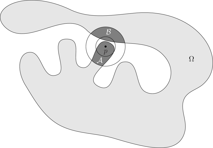
2.2: Geodesic distance example

Furthermore, we shall assume that our time steps are discrete. We denote by $\sigma(a,t)$ the pheromone level of point $a\in\Omega$ at time instance $t$, where $t=0,1,2,3,\ldots$.

2.2 The Mark-Ant-Walk (MAW) Algorithm

Initially, we consider the case where no point is marked with the pheromone, thus all $\sigma$ values are assumed to be equal to zero:

$$\sigma(a,0)=0;\ \forall a\in\Omega.$$ (2.3)

Suppose further that a starting point is (randomly) chosen for a (single) robot and then a MAW step rule (as described in Table LABEL:tab:MAW_Rule) is applied repeatedly. Note that there is no explicit stopping condition for this algorithm; nevertheless, one can use an upper bound (that will be provided later in this paper) on the cover time in order to stop robots after a sufficient time period has elapsed that effectively guarantees complete covering.

Mark-Ant-Walk step rule (current time is $t$ and robot location is $p$)
(1)	Find $x$ := a point in $R(r,2r,p)$ with minimal value of $\sigma(x,t)$
	(In case of a tie, i.e., when the minimal value achieved at several places - make an arbitrary decision
	/* note that $\|p-x\|\geq r$ */
(2)	If $\sigma(p)\leq\sigma(x)$ then $\forall u\in D(r,p)$ set $\sigma(u)=\sigma(x)+1$
	/* we mark open disk of radius $r$ around current location */
(3)	$t:=t+1$
(4)	move to $x$

2.3: MAW step rule

It is easy to see that the robot markings create some kind of potential field, where high values of the pheromone level roughly indicate areas that have been visited many times up to the moment and lower values of the pheromone level correspond to a smaller number of robot’s visits (we say “roughly indicate” because there is no strict correspondence between the pheromone level and the number of the robot visits, since marking (setting a new pheromone level) does not necessarily happen in every step). According to the MAW rule, the robot tries to avoid areas with high pheromone values by moving toward lower levels, striving to reach areas yet uncovered.

3 Related Work

In this chapter we shall discuss previous work that is close to our paradigm, i.e., we shall review the history of the “pheromone-powered” algorithms.

A step toward a “pheromone-marking”-oriented model was taken by Blum and co-workers  [Blum and Sakoda (1977), Blum and Kozen (1978)] where pebbles were used to assist the search. Pebbles are tokens that can be placed on the ground and later removed. The idea of using pebbles for unknown graph exploration and mapping was further developed in [Bender et al. (1998)].

3.1 Discrete Domains Covering Problem

Covering of discrete domains (graphs) is an important problem theoretical computer science and thus a number of solutions have been proposed and comprehensively analyzed by researchers. Well known examples are the Breadth-First Search (BFS) and the Depth-First Search (DFS) algorithms for graph traversal. Both algorithms provide excellent results in terms of time complexity. Formal proofs of complete coverage and efficiency analysis can be found in books on discrete mathematics and algorithms (see, e.g., [Rivest and Leiserson (1990)]). Note that the DFS algorithm can be readily adapted to fit our robot model as opposed to the BFS algorithm which requires additional on-board memory in order to maintain a queue of already discovered, but yet unvisited vertices. Moreover, the amount of on-board memory required depends on the graph to be explored.

Two further algorithms that fit our paradigm entirely, i.e. they relay on a group of identical autonomous robots that mark the ground with pheromones, were suggested for efficient and robust graph covering. One, called the Edge-Ant-Walk, marks the graph edges [Wagner et al. (1996)]. Another one, called the Vertex-Ant-Walk, leaves marks on graph vertices instead [Yanovski et al. (2001), Wagner et al. (1998)]. Both algorithms provided significant improvement over DFS in terms of robustness along with quite efficient cover times. Both are capable of completing the traversal of the graph in multi-robot cases even in the case when almost all robots die and/or the environment graph changes (edges/vertices are added or deleted) during the execution.

3.2 Continous Domains Covering Problem

Covering continuous domains is a relatively new problem. Several algorithms addressing this problem are summarized in a good survey paper by Choset [Choset (2001)]. We shall provide below a short review of algorithms developed for robot models that are close to the one used in this thesis.

3.2.1 Random Walk and Probabilistic Covering

Random walks were defined for both discrete and continuous domains and enjoy unrivaled robustness and scalability; however, they cannot guarantee complete coverage and can be analyzed in terms of expected coverage time only. We would like to have solutions that guarantee complete coverage after a deterministic and bounded time period.

3.2.2 Motion Planning Guided by a Potential Field

A very popular approach is to introduce an artificial potential field concept in order to accomplish the robot motion planning task (e.g. [Khatib (1986), Zelinsky et al. (1993)]). In [Zelinsky et al. (1993)], for example, the authors used the distance transform as the potential field. Such an approach could also be adopted by our robots, the potential being represented by the odor level. However, this type of work assumed that the potential field can be constructed prior to the start of robot’s motion and thus requires a global knowledge of the domain boundaries and obstacles. Such knowledge is not available in our model. However, similar results could be achieved if we assumed that obstacles were actually the pheromone source and that the odor level decreases gradually as we move away from them thereby forming some kind of distance transform.

3.2.3 Trail Lying Algorithms for Continuous Domains

Several authors proposed to use trails that mark the path traveled by the robot so far, and proposed local behavior for the robots that resulted in some kind of peeling/milling of the domain. Here two major approaches for organizing the motion exist: contour-parallel and direction-parallel. In the former approach, the robot moves along the boundaries of the domain; in the latter one, the robot moves back and forth in some predefined direction. These approaches often fail for non-convex domains and thus the whole domain must be approximated as a union of convex non-overlapping cells, which, in turn, can be covered with the assumed type of motion [Choset and Pignon (1997), Butler (2000), Acar et al. (2003)]. Another representative of trail-based algorithms is the Mark-And-Cover (MAC) algorithm presented in [Wagner et al. (2000)], which is actually an adaptation of the DFS algorithm to continuous domains. This algorithm provides efficient and effective coverage with a provable bound on cover time. Additionally, the robot model used in the paper fits our paradigm very well. Nevertheless, the drawback of the MAC algorithm, and, in fact, of all trail-based algorithms, is their sensitivity to noise and robot failure. Moreover, in the multi-robot case trails of the robots interfere with the motion of the others and may hamper their efficiency. Another shortcoming of these algorithms is seen in the situation when the domain is required to be covered repeatedly, e.g., in surveillance tasks or in the scenario described in [Gage (1994)] where autonomous robots are used to de-mine minefields using imperfect sensors (in the sense that the probability of a mine detection is less than 1). Our algorithm guarantees that the whole domain is covered repeatedly, time after time. Furthermore, the time between two successive visits at any point can be bounded in terms of the (unknown) size of the problem (see Section LABEL:sec:repetitive-coverage).

3.2.4 Tessalating Algorithms for Continuous Domains

Another possible approach is to split the domain into tiles such that each tile is easily covered by the robots (e.g., convex tiles are suitable for “onion peeling” or “back and forth” algorithms). After a particular tile is covered, the robot goes to a new one that is a neighbor of the current tile. This approach, in fact, takes us back to a graph covering of an underlying graph whose vertices are associated with the tiles, the edges between vertices being defined according to the inter-tile connectivity.

4 The MAW Algorithm: Formal Proof and Efficiency Analysis

4.1 MAW - Proof of Complete Coverage

Let us first show that a single robot governed by the MAW rule covers any connected bounded domain in a finite number of steps. The outline of the proof is as follows.

First, we prove that at any time instance, any two points that are close enough, i.e., their distance from each other is less than or equal to $r$, must have pheromone levels that differ by one at most. This property closely resembles Lipschitz continuity for functions $f(\cdot)$:

$$|f(p_{1})-f(p_{2})|\leq\kappa\|p_{1}-p_{2}\|,$$ (4.1)

for some constant $\kappa$. However, our $\sigma$ function measuring the level of the pheromone at each location is, by definition, not continuous and thus cannot be Lipschitz continuous. Instead, $\sigma$ obeys the following inequality:

$$|\sigma(p_{1})-\sigma(p_{2})|\leq\kappa\|p_{1}-p_{2}\|+1.$$ (4.2)

We call this the proximity principle, and it has also been used in several previous papers [Yanovski et al. (2001), Wagner et al. (1996), Wagner et al. (1998)].

Second, we look at the diameter $d$ of the domain, defined as the length of the longest geodesic path that can be embedded in the domain: consider a pair of points $a,b\in\Omega$. Since $\Omega$ is connected, there is at least one path that connects $a$ and $b$ and lies entirely in the domain $\Omega$. Among all such paths (connecting $a$ and $b$, that are restricted to lie entirely in the domain $\Omega$), there is at least one that is the shortest. We call the length of this shortest path the distance between $a$ and $b$ and denote it by $\|a-b\|$. Among all possible pairs of points $a,b\in\Omega$, there exists a pair $(a_{0},b_{0})$ that has the greatest possible distance between them, i.e.,

$$\|a_{0}-b_{0}\|\geq\|a-b\|\;\forall a,b\in\Omega.$$ (4.3)

We call the length of this longest geodesic path the diameter of the domain and denote it by $d$. In other words:

$$d\triangleq\sup_{(a,b)\in\Omega}\|a-b\|.$$ (4.4)

Assuming that $d$ is finite (actually the requirement that the domain $\Omega$ is bounded is related to its diameter and its perimeter), we easily conclude with the aid of the proximity principle that, at any time $t$ for any two points $a,b\in\Omega$, the difference between the pheromone levels of these two points is upper bounded by $\lceil d/r\rceil$. This, in turn, means that once a value of $\lceil d/r\rceil+1$ is reached by $\sigma()$ at any point, no unmarked point may exist and thus the whole domain has been covered by the robot. Finally, we show that the maximal pheromone marker value goes to infinity as time goes to infinity hence we shall surely, at some time reach the value of $\lceil d/r\rceil+1$. Formal proofs are given below.

Lemma 1.

The difference between marker values of near by points is bounded.

$$\forall t;\forall a,b\in\Omega\text{ : if }\|a-b\|\leq r\text{ then }|\sigma(a,t)-\sigma(b,t)|\leq 1$$

Proof:

Note that the distance $\|a-b\|$ is the length of the shortest path between these two points, which is restricted to lie entirely in the domain $\Omega$. We shall prove the lemma by mathematical induction on the step number. The lemma is clearly true at $t=0$ when all the marks are assumed to be zero. Assuming it is also true at time $t$, we shall show it remains true at time $t+1$. Let us look at two arbitrary points $a,b\in\Omega$, such that $\|a-b\|\leq r$. In the trivial case neither $a$ nor $b$ change their marker values at the $(n+1)$th step; therefore, the lemma continues to hold. If both $a$ and $b$ change their values, then $\sigma(a,t+1)=\sigma(b,t+1)$ since the algorithm assigns the same values to all the points it changes. Hence the only interesting case is when only one point (say $a$) changes its marker value, while the other one remains unchanged. Assuming the current robot’s location is $p_{t}$ we conclude that $a$ belongs to $D(r,p_{t})$, otherwise it could not change its marker value. Therefore, $\|a-p_{t}\|<r$. However, $b$ does not change its marker value and thus $\|b-p_{t}\|\geq r$. Combining these constraints we get:

$$\left\{\begin{array}[]{l}\|a-b\|\leq r\\ \|a-p_{t}\|\leq r\\ \|b-p_{t}\|\geq r\end{array}\right.\Rightarrow r\leq\|b-p_{t}\|\leq 2r,$$ (4.5)

or, equivalently, $b\in R(r,2r,p_{t})$. This situation is depicted in Figure LABEL:fig:proximity. Now let us recall how the new marker value of $a$ is determined. First, we look for the minimal marker value among all points in $R(r,2r,p_{t})$. Assume that this value is attained at some point $x\in R(r,2r,p_{t})$. The new marker value of $a$ is then set if and only if the pheromone level at the current robot’s location is smaller than or equal to that at $x$: $\sigma(p_{t},t)\leq\sigma(x,t)$. In this case we have:

$$\sigma(a,t+1)=\sigma(x,t)+1.$$ (4.6)

Since both points $x$ and $b$ belong to $R(r,2r,p_{t})$, we have

$$\sigma(b,t)\geq\sigma(x,t),$$ (4.7)

because of the way the point $x$ was chosen. Now, on the one hand, we have:

$$\left\{\begin{array}[]{l}|\sigma(a,t)-\sigma(b,t)|\leq 1\\ \sigma(b,t)\geq\sigma(x,t)\end{array}\right.\Rightarrow\sigma(a,t)\geq\sigma(x,t)-1;$$ (4.8)

and on the other hand:

$$\left\{\begin{array}[]{l}|\sigma(a,t)-\sigma(p_{t},t)|\leq 1\\ \sigma(p_{t},t)\leq\sigma(x,t)\end{array}\right.\Rightarrow\sigma(a,t)\leq\sigma(x,t)+1.$$ (4.9)

Combining inequalities (LABEL:eq:sigma_a_big) and (LABEL:eq:sigma_a_small), we get

$$|\sigma(a,t)-\sigma(x,t)|\leq 1.$$ (4.10)

Using the system of inequalities (LABEL:eq:sigma_a_big), we conclude that

$$0\leq\sigma(b,t)-\sigma(x,t)\leq 2.$$ (4.11)

Combining the above inequality with the fact that $\sigma(a,t+1)=\sigma(x,t)+1$ and $\sigma(b,t+1)=\sigma(b,t)$, we get the desired result:

$$|\sigma(a,t+1)-\sigma(b,t+1)|\leq 1.$$ (4.12)

Thus the lemma is proved.  

4.1: Close points have close marker values

Lemma 2.

The difference between marker values of any two points is bounded at any time instance.

$$\forall t;\forall a,b\in\Omega\text{ : }|\sigma(a,t)-\sigma(b,t)|\leq\left\lceil\frac{d}{r}\right\rceil,$$

where $d$ is the diameter of $\Omega$.

Proof:

Let us consider a path connecting the points $a$ and $b$. We can always split the path into sub-paths of length $r$, as depicted in Figure LABEL:fig:proximity_global. According to Lemma LABEL:lem:close_points difference between the marker values at the endpoints of every such sub-path is limited by 1, hence, we can conclude that

$$|\sigma(a,t)-\sigma(b,t)|\leq\left\lceil\frac{l}{r}\right\rceil,$$ (4.13)

where $l$ represents the length of the path. Obviously, among all paths connecting $a$ and $b$ the shortest path will provide best upper bound on the difference between the pheromone levels at $a$ and at $b$. Since the longest geodesic path in $\Omega$ is limited by $d$ we obtain the desired result:

$$|\sigma(a,t)-\sigma(b,t)|\leq\left\lceil\frac{d}{r}\right\rceil.$$ (4.14)

 

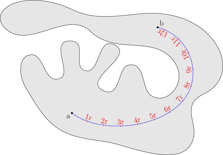
4.2: Difference between marker values of any two points is bounded.

It is implied by Lemma LABEL:lem:max_diff that the difference between marker values is bounded. Our next step will be to show that the maximal marker value tends to infinity as $t$ goes to infinity. First, we prove that marker values can only grow and never decrease.

Lemma 3.

Pheromone level values at any point form a non-decreasing sequence. That is

$$\forall t;\forall u\in\Omega\text{ : }\sigma(u,t+1)\geq\sigma(u,t).$$

Proof:

Let us assume the contrary, i.e., there exists a point $u\in\Omega$ and time instance $t$ such that the pheromone level of $u$ decreases during the $t$-th step:

$$\sigma(u,t+1)<\sigma(u,t).$$ (4.15)

Let us now look at point $p_{t}$ – the location of the robot at time $t$. Obviously $u$ belongs to $D(r,p_{t})$ (otherwise it could not change its value), hence $\|u-p_{t}\|<r$. Assume that the minimal marker value among all points in $R(r,2r,p_{t})$ was attained at some point $x$. We know also that $\sigma(p_{t},t)\leq\sigma(x,t)$; otherwise, the robot does not change the pheromone values. Thus we have

$$\left\{\begin{array}[]{l}\sigma(x,t)+1=\sigma(u,t+1)<\sigma(u,t)\\ \sigma(p_{t},t)\leq\sigma(x,t)\\ \|u-p_{t}\|<r\end{array}\right.$$ (4.16)

This implies

$$\left\{\begin{array}[]{l}|\sigma(u,t)-\sigma(p_{t},t)|>1\\ \|u-p_{t}\|<r\end{array}\right.$$ (4.17)

which contradicts Lemma LABEL:lem:close_points.  

Next, we show that the maximal value of the pheromone level grows together with the step number $t$.

Lemma 4.

At any time instance $t$ maximal pheromone level in $\Omega$ is bounded from below by $t/n$ for some constant $n$.

Proof:

Imagine that the domain $\Omega$ is tessellated into $n$ cells so that the diameter of every such cell is less than $r$ (for convex cells we can, alternatively, require that the diameter of the circumscribing circle must be less than $r$). Let us examine the following expression:

$$S_{t}=\sum_{i=1}^{n}m_{t}^{i}-\sigma(p_{t},t),$$ (4.18)

where $m_{t}^{i}$ is the minimal marker value over the $i$th cell at time $t$ and $\sigma(p_{t},t)$ is the marker value at the robot’s location $p_{t}$ at time instance $t$. It was shown in Lemma LABEL:lem:non_decreasing that marker values of any point inside $\Omega$ form a non-decreasing sequence. Hence we claim that

$$S_{t+1}>S_{t}.$$ (4.19)

Indeed, for the non-marking step, the sum of the minima does not change: $\sum_{i=1}^{n}m_{t}^{i}=\sum_{i=1}^{n}m_{t+1}^{i}$; however $\sigma(p_{t},t)>\sigma(p_{t+1},t+1)$, and therefore, $S_{t+1}>S_{t}$. For the marking step, assuming that the robot goes from cell $k$ into cell $l$, we have $\sigma(p_{t},t)\leq\sigma(p_{t+1},t+1)$, and therefore, $m_{t}^{k}\leq\sigma({p_{t+1},t+1})$. Additionally, the whole cell $k$ was marked during this step and thus $m_{t+1}^{k}=\sigma(p_{t+1},t+1)+1$. Hence we have

$$\left\{\begin{array}[]{l}m_{t}^{k}-\sigma(p_{t},t)\leq 0\\ m_{t+1}^{k}-\sigma(p_{t+1},t+1)=1.\end{array}\right.$$ (4.20)

Since the sum of the other minima cannot decrease as was shown in Lemma LABEL:lem:non_decreasing, we conclude again that $S_{t+1}>S_{t}$. Given that $S_{0}=0$, we readily conclude that

$$S_{t}\geq t\Rightarrow\sum_{i=1}^{n}m_{t}^{i}\geq t\quad\forall t,$$ (4.21)

which leads us to the conclusion that there exists $k\in 1,2,\ldots,n$ such that

$$m^{k}_{t}\geq\frac{t}{n}.$$ (4.22)

Hence the lemma is proved.  

At this point we are ready to prove the main result of this work.

Theorem 1.

The domain $\Omega$ will be covered within a finite number of steps.

Proof:

According to Lemma LABEL:lem:max_growth after $n\lceil\frac{d}{r}\rceil+1$ steps, at least one of the $m^{i}$ values will be greater than $\lceil\frac{d}{r}\rceil$ and thus the whole domain will be covered.  

4.2 MAW - Efficiency Analysis

As we proved earlier the domain $\Omega$ will be covered by a single robot after $n\lceil\frac{d}{r}\rceil+1$ steps where $d$ is the diameter of the domain, $r$ - the covering radius of the robot’s effector and $n$ - the number of cells in some tessellation of $\Omega$ (see Lemma LABEL:lem:max_growth for the definition of $n$). We shall now analyze how good this upper bound is. In order to make such comparison we shall find an approximation to $n$ and to find out what is the best upper bound possible.

Let us denote by $N_{r}$ the minimal number of steps required by the robot to cover the whole domain $\Omega$ (here we only assume that the robot can cover an open disk of radius $r$ at every step, however, no assumption is made regarding the algorithm governing the robot’s behavior). Clearly $N_{r}=\frac{A_{\Omega}}{a_{r}}$, where $A_{\Omega}$ and $a_{r}$ are the areas of the domain $\Omega$ and robot’s effector respectively. Obviously, this is an ultimate lower bound and no algorithm can beat it. However this bound fails be tight enough for domains whose shape factor (ratio of the squared domain perimeter to its area multiplied by $4\pi$) is far from 1 (not round). For example, domains, comprised of finite number of curves and line segments would have zero area providing lower bound to be zero, which is, of course, meaningless. As a possible solution, in [Wagner et al. (2000)] the authors used the area of the “augmented” domain $\bar{\Omega}$, which results from an inflation or expansion $\Omega$ in all directions by $r$ , i.e., $\Omega$ has undergone a morphological dilation with a disk of radius $r$. In this case we have [Wagner et al. (2000)]:

$$A_{\bar{\Omega}}\leq A_{\Omega}+rP_{\Omega}+\pi r^{2},$$ (4.23)

where $A_{\Omega}$ and $P_{\Omega}$ are the area and the perimeter of $\Omega$, respectively. This approach has a serious drawback: there are situations when the augmented domain can be covered by the robot in a finite number of steps while the original domain can not. As an illustration of such domain consider a star-shaped domain comprised of a number of line segments, say of length $r$, emanating from a common origin, as shown in Figure LABEL:fig:star_shaped. Obviously, the number of line segments can be infinite and since we cover an open dist of radius $r$ in each step we will be forced to “enter” into every such line segment in order to cover it completely and thus the number of step required to cover such a domain will also be infinite. Note, however, that the augmented domain in this case can be covered in a finite number of steps.

4.3: A “pathological” star shaped domain.

We suggest another way of performance assessment which is correct by construction and does not depend on geometric properties like area or perimeter. Consider best possible algorithm that covers in each step an open disk of radius $r/2$, besides this requirement we do not limit the algorithm in any other way. Assume that the our domain $\Omega$ can be covered by such algorithm. That is there exists a finite sequence of points $P_{1},P_{2},\ldots P_{N}$ of robot’s locations that results in complete coverage, that is :

$$\Omega\subset\bigcup_{i=1}^{N}D\left(\frac{r}{2},P_{i}\right).$$ (4.24)

Alternatively, we can say that for every point $a$ in $\Omega$ there exist a number $k$ ($1\leq k\leq N$) such that $a\in D(r/2,P_{k})$. Now, if we consider the best possible algorithm, as before we denote its coverage time by $N_{r/2}$, we easily conclude that the upper bound on the number of steps required by MAW algorithm is:

$$N_{r/2}\left\lceil\frac{d}{r}\right\rceil+1.$$ (4.25)

Indeed, if we consider a particular coverage path or the robot described by the sequence of its successive positions: $P_{1},P_{2},\ldots P_{N_{r/2}}$ we always can perform Voronoi tessellation around these points. Each cell in this tessellation will have diameter smaller than $r$ and thus this tessellation will be like the one we used in Lemma LABEL:lem:max_growth.

We have only to estimate the $d/r$ fraction. Obviously, $\frac{d}{r}\leq N_{r/2}$ on one hand, on the other hand we can estimate the lower bound: $\frac{d}{r}\geq\frac{\pi}{4}\sqrt{N_{r/2}}$ (for domains that have a shape close to a circle). Hence we have shown that the upper bound time is polynomial with respect to best possible time of algorithm whose covering radius is $r/2$.

$$t_{\mathrm{coverage}}\leq N_{r/2}^{x},$$ (4.26)

where $0.5\leq x\leq 2$.

The main question here is whether we can conclude that

$$t_{\mathrm{coverage}}\leq N_{r}^{x},$$ (4.27)

i.e., whether our coverage time is bounded by a polynomial function of $N_{r}$, which is best possible coverage time among all algorithms whose covering radius is $r$. The general answer is “No”. In fact, a general theorem regarding limitations of such a type of algorithms:

Theorem 2.

Given an algorithm whose marking area is an open disk of radius $r$ and step size is grater than or equal to $r$. The time for complete coverage $t_{\mathrm{coverage}}$ of a continuous domain is (tightly) limited from below by $N_{r/2}$. Moreover $t_{\mathrm{coverage}}$ cannot be expressed as a bounded function of $N_{x}$ for any $x>r/2$.

Proof:

The proof is by example of such a domain: we consider again a domain comprised of $n$ line segments emanating common origin $O$, as shown if Figure LABEL:fig:star_shaped. Assuming that the length of each line segment is $r/2$ we easily verify that $N_{r/2}=n$ and that $t_{\mathrm{coverage}}=n$ (assuming that the robot’s initial position was an end-point of any line segment. Hence $t_{\mathrm{coverage}}$ is (tightly) bounded from below by $N_{r/2}$. Now if we assume that $n$ is infinite we easily conclude that such domain cannot be covered in a finite number of steps by our algorithm (again, provided that the initial robot location was at an end point of any line segment), while this domain can be covered in two steps by an optimal algorithm whose covering radius is greater than $r/2$ (we simply go to the origin $O$ in the very first step and the whole domain will be covered in the next step). Hence, the theorem is proved.  

Of course the above theorem is quite general, for a particular domain one can have

$$N_{r}\propto N_{r/2},$$ (4.28)

hence, best possible time would be linear in terms of $N_{r}$ and MAW’s coverage time would be limited from above by $N_{r}^{2}$ times some constant.

Let us elaborate more about the relationship between $N_{r}$ and $N_{r/2}$. Consider a domain of area $A$ and perimeter $P$. Consider also an optimal coverage with radius $r$. According to our definitions this coverage requires exactly $N_{r}$ steps. Let us now look at the Voronoi tessellation around corresponding robots’ locations, there are $N_{r}$ cells in this tessellation. Cells that do not include the boundary of the domain are convex, those that do include domain’s boundaries may not be convex. Each convex cell in this tessellation can be covered by a finite (and well-defined) number of disks of radius $r/2$, hence for these cells we can conclude that $N_{r}\propto N_{r/2}$. For non-convex cells this claim may not be correct, thus, for domains whose tessellation consists mainly of convex cells we have approximately $N_{r}\propto N_{r/2}$. Note that a similar analysis was carried out on the MAC algorithm [Wagner et al. (2000)] where the authors claim that MAC algorithm is asymptotically linear for domains that obey $A>>Pr$. This is, fact, equivalent to say that the number of cells in the Voronoi tessellation described above that do not contain domain’s boundary is large compared to the number of the cells that do.

5 Extensions

5.1 Repetitive Coverage

In some scenarios we might be interested in repetitive coverage of the domain. For example, repetitive coverage is necessary in the aforementioned scenario when robots perform minefield de-mining and their mine detection is not perfect, i.e., the probability of detecting a mine when the robot’s sensors sweep above it is less than one. In this case repetitive coverage is required to minimize the probability of leaving any mines undetected. In this case, we have to give an upper bound on time between two successive visits of the robot in order to guarantee an improvement in detection probability. This requirements also arises naturally in tasks such as surveillance or patrolling where robots are required to visit every point over and over and the time between two successive visits must be limited by a constant. In other word we shall show now that our algorithm has the property of patrolling. Before we start proving this result we shall need the following lemma.

Lemma 5.

For any two time instances $t_{1}$ and $t_{2}$, if $t_{2}>t_{1}$ then the following inequality must hold:

$$S_{t_{2}}-S_{t_{1}}\geq t_{2}-t_{1}.$$

Proof:

Let us write $t_{2}=t_{1}+n$ for some natural $n$ and prove the lemma by mathematical induction on $n$. For $n=1$ the lemma holds due to Equation (LABEL:eq:growth_sum). Assuming that the lemma holds for some $n$, we can easily conclude that the lemma holds for $n+1$ as well.  

Theorem 3.

For any point $a\in\Omega$, the time period between two successive visits of the robot is bounded from above by

$$2n\left(\left\lceil\frac{d}{r}\right\rceil+1\right)$$

.

Proof:

If we show that after a sufficient time period the pheromone level changes at all locations in the domain $\Omega$, we can obviously be sure that all points were re-visited by the robot during this time period. Let us look at time instance $t_{s}$ when the robot covers our point of interest $a$. We denote by $\sigma_{max}(t_{s})$ the maximal pheromone level over $\Omega$ at that time. If we show that at some time instance $t_{e}$ the minimal pheromone level denoted by $\sigma_{min}(t_{e})$ becomes greater than the maximal value that was at time $t_{s}$:

$$\sigma_{min}(t_{e})>\sigma_{max}(t_{s}),$$ (5.1)

then we can easily conclude that during the time period $t_{e}-t_{s}$ the pheromone level changed at all points and thus all points (including $a$) were re-covered by the robot. Let us examine $S_{t_{s}}$ and $S_{t_{e}}$ as defined in the Equation (LABEL:eq:min_sum). On the one hand:

$$S_{t_{s}}=\sum_{i}^{n}m^{i}_{t_{s}}-\sigma(p_{t_{i}},t_{i})\geq\sum_{i}^{n}m^{i}_{t_{s}}\geq\sum_{i}^{n}\sigma_{min}(t_{s})=n\,\sigma_{min}(t_{s})$$ (5.2)

According to Lemma LABEL:lem:max_diff

$$\sigma_{min}(t_{s})\geq\sigma_{max}(t_{s})+\left\lceil\frac{d}{r}\right\rceil.$$ (5.3)

Combining Equations (LABEL:eq:8) and (LABEL:eq:9) we get

$$S_{t_{s}}\geq n\left(\sigma_{max}(t_{s})-\left\lceil\frac{d}{r}\right\rceil\right).$$ (5.4)

On the other hand we want to know the time instance $t_{e}$ that guarantees that $\sigma_{min}(t_{e})\geq\sigma_{max}(t_{s})+1$. Instead of estimating $t_{e}$ directly from $\sigma_{min}(t_{e})$, we shall look for $t_{e}$ that guarantees the existence of $\sigma$ value greater than or equal to $\sigma_{max}(t_{s})+1+\lceil\frac{d}{r}+1\rceil$, which guarantees by Lemma LABEL:lem:max_diff that $\sigma_{min}(t_{e})\geq\sigma_{max}(t_{s})+1$. Now, in the same way as the proof of Theorem LABEL:theo:the_one, we can say that once $S_{t_{e}}\geq n(\sigma_{max}(t_{s})+1+\lceil\frac{d}{r}\rceil+1)$, we have $\sigma_{min}(t_{e})\geq\sigma_{max}(t_{s})+1$. Thus we have

$$S_{t_{e}}-S_{t_{s}}\leq n\left(\sigma_{max}(t_{s})+1+\left\lceil\frac{d}{r}\right\rceil+1\right)-\left(\sigma_{max}(t_{s})-\left\lceil\frac{d}{r}\right\rceil\right)\\ =2n\left(\left\lceil\frac{d}{r}\right\rceil+1\right).$$ (5.5)

According to Lemma LABEL:lem:sum_to_time we have

$$t_{e}-t_{s}\leq S_{e}-S_{s}\leq 2n\left(\left\lceil\frac{d}{r}\right\rceil+1\right),$$ (5.6)

which completes the proof.  

We now make two important observations. First, the upper time bound between two successive visits by the robot does not depend on the current pheromone level distribution. This is determined completely by the geometric parameters of the problem: $r$, $n$, and $d$. Second, we observe that this time limit is twice as long as the time period needed for complete coverage. This situation is quite intuitive. Indeed, observe the pheromone level along some path in $\Omega$, such as the one shown in Figure LABEL:fig:recovered-a. In this case the robot may start by “filling” the hollow area on the right until it becomes a hill and only then covers the left-hand part, which used to be a summit point and has now became the lowest point in the pheromone level profile as shown in Figure LABEL:fig:recovered-b.

(a) Pheromone level along some path in $\Omega$.

(b) The worst case that guarantees that the whole domain was re-covered.

5.1: Repetitive coverage illustration

5.2 Noise Immunity

So far we always assumed that there is no noise in the input, i.e., the robot starts with a domain that does not contain any pheromone marks. Unfortunately, in the real life such a clean environment is not always available. For example, spurious pheromone marks may arise as a result of previous attempts to explore the domain by similar robots, which might have used other algorithms and thus the initial pheromone level distribution does not necessarily obey the proximity principle. In general we assume that the initial pheromone level distribution is given by some function

$$N:\Omega\mapsto\mathbb{Z}^{*},$$ (5.7)

where $\mathbb{Z}^{*}$ denotes the set of non-negative integers. As a short digression we have to note that such initial pheromone marks pose a severe problem to all trail-based algorithms. The reason is that such algorithms, for the sake of efficiency, do not get close to their own trails and thus any initial pheromone marks would be interpreted as trails, resulting in uncovered areas around such marks. The result may be even worse if such false trails split the domain into several disconnected parts, in this case the robot will not be able to exit the part where it was located initially. Our algorithm, on the contrary, can easily overcome this problem as we prove below. Actual covering times in presence of noise are demonstrated in Section LABEL:sec:maw-noisy-envir. Let us start with several lemmas.

Lemma 6.

Immediately after point $a\in\Omega$ has been marked by the robot for any point $b\in\Omega$ such that $\|a-b\|\leq r$ we have:

$$\sigma(b,t+1)\geq\sigma(a,t+1)-1,$$ (5.8)

where $t$ denotes the time instance when the new pheromone level was assigned to $a$.

Proof:

Since the pheromone value of $a$ changes during the $t$th step we conclude that $a\in D(r,p_{t})$, where $p_{t}$ denotes robot’s location at time $t$. We know also that $\|a-b\|\leq r$ and thus $b$ either belongs to $D(r,p_{t})$ or to $R(r,2r,p_{t})$ (see Figure LABEL:fig:noise_proximity1). Hence there are two possible scenarios: either $b$ belongs to $D(r,p_{t})$ or $b$ belongs to $R(r,2r,p_{t})$. In the former case $\sigma(b,t+1)=\sigma(a,t+1)$ since the algorithm assigns the same value to all points in $D(r,p_{t})$ and the lemma clearly holds. In the latter case ($b\in R(r,2r,p_{t})$) we recall that the algorithm seeks for the minimal pheromone value inside $R(r,2r,p_{t})$, say attained at some point $x$ and set new pheromone level inside $D(r,p_{t})$ to be equal to $\sigma(x,t)+1$. Hence, we have:

$$\left\{\begin{array}[]{l}\sigma(b,t+1)=\sigma(b,t)\geq\sigma(x,t)\\ \sigma(a,t+1)=\sigma(x,t)+1\end{array}\right..$$ (5.9)

This leads us again to the conclusion

$$\sigma(b,t+1)\geq\sigma(a,t+1)-1.$$ (5.10)

Hence the lemma is proved.  

5.2: Close points in noisy environment

Though this lemma resembles Lemma LABEL:lem:close_points, it does not guarantee that the proximity principle is obeyed in noisy environment. We demonstrate a stronger result later in Lemma LABEL:lem:noise-immunity-2.

At this moment we shall prove that the pheromone level at marked points, i.e., pheromone left by the robot never decreases.

Lemma 7.

Pheromone level values at any marked point form a non-decreasing sequence; that is

$$\forall t\;\forall u\in\Omega:\sigma(u,t+1)\geq\sigma(u,t)$$

given that $u$ was marked by the robot at the time prior to $t$.

Proof:

Let us assume the contrary, i.e., for some time instance $t$ and for some point $u\in\Omega$ we have:

$$\sigma(u,t)<\sigma(u,t+1)$$ (5.11)

Let $t$ be the first such time instance. As usual we denote by $p_{t}$ the robot’s location at time $t$. According to the MAW algorithm the robot seeks to the minimal pheromone level in $R(r,2r,p_{t})$. Say this minimal level is attained at some point $x\in R(r,2r,p_{t})$. Since $u$ changes its value during the $t$th step we conclude that

$$\sigma(p_{t},t)\leq\sigma(x,t).$$ (5.12)

Otherwise no change happens, according to the MAW algorithm. Sine all points in $D(r,p_{t})$ get the same value in the marking step we conclude:

$$\sigma(u,t+1)=\sigma(p_{t},t+1)=\sigma(x,t)+1\geq\sigma(p_{t},t)+1$$ (5.13)

Moreover, according to our assumption:

$$\sigma(u,t)>\sigma(u,t+1)\Rightarrow\sigma(u,t)\geq\sigma(p_{t})+2.$$ (5.14)

Thus, if we assume that the pheromone level at some point $u$ decreases at time instance $t$ Equation (LABEL:eq:25) must hold. Showing that this inequality is wrong we actually get a contradiction to the assumption and thus prove the lemma. Let us look at the time instance $t_{u}$ when the current pheromone level of $u$ ($\sigma(u,t)$) was set. According to Lemma LABEL:lem:noise-immunity-1:

$$\sigma(p_{t},t_{u}+1)\geq\sigma(u,t_{u}+1)-1.$$ (5.15)

Since $t_{u}<t$ and $t$ was chosen to be the first time when the pheromone level at any point in $\Omega$ decreases we conclude that

$$\sigma(p_{t},t)\geq\sigma(p_{t},t_{u}+1).$$ (5.16)

Substituting it into Equation (LABEL:eq:28) we get

$$\sigma(p_{t},t)\geq\sigma(u,t)-1.$$ (5.17)

And thus, the inequality in Equation (LABEL:eq:25) does not hold. This contradiction completes the proof of the lemma.  

Lemma 8.

If, at some time instance $t$, both $a$ and $b$ had been marked by the robot their pheromone levels obey the proximity principle,i.e.,

$$\text{if }|a-b|\leq r,\text{ then }|\sigma(a,t)-\sigma(b,t)|\leq 1$$ (5.18)

Proof:

Since both $a$ and $b$ had been marked prior to time instance $t$ there are exist time instances $t_{a}$ and $t_{b}$ when $a$ and $b$ got their current pheromone levels accordingly. Applying Lemma LABEL:lem:noise-immunity-1 we get the following two equations:

$$\left\{\begin{array}[]{l}\sigma(b,t_{a}+1)\geq\sigma(a,t_{a}+1)-1\\ \sigma(a,t_{b}+1)\geq\sigma(b,t_{b}+1)-1.\end{array}\right.$$ (5.19)

Or, substituting $\sigma(b,t_{b}+1)=\sigma(b,t)$ and $\sigma(a,t_{a}+1)=\sigma(a,t)$

$$\left\{\begin{array}[]{l}\sigma(b,t_{a}+1)\geq\sigma(a,t)-1\\ \sigma(a,t_{b}+1)\geq\sigma(b,t)-1.\end{array}\right.$$ (5.20)

Since $t>t_{a}$ and $t>t_{b}$ we can apply Lemma LABEL:lem:noise-immunity-3:

$$\left\{\begin{array}[]{l}\sigma(b,t)\geq\sigma(b,t_{a}+1)\\ \sigma(a,t)\geq\sigma(a,t_{b}+1).\end{array}\right.$$ (5.21)

Substituting it into Equation LABEL:eq:33 we get

$$\left\{\begin{array}[]{l}\sigma(b,t)\geq\sigma(a,t)-1\\ \sigma(a,t)\geq\sigma(b,t)-1.\end{array}\right.$$ (5.22)

Which means

$$|\sigma(a,t)-\sigma(b,t)|\leq 1$$ (5.23)

Hence the lemma is proved.  

Lemma 9.

The maximal pheromone level tends to infinity as $t$ goes to infinity.

Proof:

The proof is identical to the one in Lemma LABEL:lem:max_growth. We again introduce a virtual tessellation of domain $\Omega$ into $n$ cells so that every such cell can be inscribed into a circle of diameter less than $r$. And, as before, we look at the sum:

$$S_{t}=\sum_{i=1}^{n}m_{t}^{i}-\sigma(p_{t},t)$$ (5.24)

The only difference that this time $m_{t}^{i}$ denotes the minimal marker value that was set by the robot and not as a result of the noise. As in Lemma LABEL:theo:the_one we get

$$S_{t}\geq t\ \forall t.$$ (5.25)

Thus the lemma is proved.  

Theorem 4.

For any initial noise profile $N:\Omega\mapsto\mathbb{Z}^{*}$, the domain $\Omega$ will be covered after $n(M_{N}-m_{N}+\lceil\frac{n}{r}\rceil)+1$ steps, where $M_{N}$ and $m_{N}$ denotes the maximal and the minimal pheromone levels at time $t=0$, respectively.

Proof:

Let us denote by $M_{N}$ and by $m_{n}$ respectively, the maximal and the minimal values of the initial pheromone level given by $N$. According to Lemma LABEL:lem:maximal2 the maximal pheromone level in $\Omega$ grows and will eventually reach the value of $M_{N}+\lceil\frac{n}{r}\rceil+1$. We claim that at this moment the whole domain is covered by the robot. Indeed, let us look at some point $a\in\Omega$ that got at step $t$ this pheromone level. According to Lemma LABEL:lem:noise-immunity-1 for any point $b\in\Omega$ such that $\|a-b\|\leq r$ we have

$$\sigma(b,t+1)\geq\sigma(a,t+1)-1=M_{N}+\left\lceil\frac{n}{r}\right\rceil.$$ (5.26)

Since $M_{N}+\lceil\frac{n}{r}\rceil>M_{N}$ we conclude that all such points are covered. In the same manner we get that all points whose distance from $a$ is less than or equal to $2r$ are also covered. And so on, maximal distance between points in$\Omega$ is bounded by $d$, thus one any point reaches pheromone level of $M_{N}+\lceil\frac{n}{r}\rceil+1$ we assure that the minimal possible pheromone level is $M_{N}+1$ which means that the whole domain $\Omega$ has been covered. The time needed to cover the domain is

$$t_{cover}=n\left(M_{N}-m_{N}+\left\lceil\frac{n}{r}\right\rceil\right)+1,,$$ (5.27)

where $m_{N}$ denotes minimal pheromone level at time $t=0$. Since the whole domain is covered we can guarantee, by Lemma LABEL:lem:noise-immunity-2 the proximity principle is obeyed by any two points in $\Omega$ and further repetitive coverage is governed by Theorem LABEL:theo:repetitive.  

5.3 Multiple Robots

As a natural extension we would like to analyze how the MAW algorithm can be applied to multi-robot environments. First of all, we must address problems such as collisions both between the robots themselves (if we deal with physical robots and not programs) and between different pheromone levels when two (or more) robots try to mark the same point in the domain.

At the moment we shall assume that the clock phases of all robots are slightly different so that no two robots are active at the same time. Thus each robot sees other robots as regular stationary obstacles and acts accordingly. With this approach we also have no problem of simultaneous attempts to set (probably different) pheromone levels at particular location by multiple robots, since only one robot is active at any given time.

Let us find the upper bound for complete coverage provided we have $n$ robots. Using the same notation as in Equation (LABEL:eq:min_sum) we have:

$$S_{t}=\sum_{i=1}^{n}m_{t}^{i}-\sum_{j=1}^{n}\sigma(p_{t}^{j},t),$$ (5.28)

where $p_{t}^{j}$ denotes the location of the $j$-th robot at time $t$. Using exactly the same reasoning as before, we again obtain:

$$S_{t+1}>S_{t},$$ (5.29)

and consequently

$$S_{t}\geq t,$$ (5.30)

which leads us to the same upper bound we got for a single robot. Hence adding more robots does not necessarily guarantees better coverage time. However simulations (see Section LABEL:sec:simul-exper) demonstrate that there is a substantial improvement when we use more robots.

5.4 Generalization for Other Metrics

Until now we always assumed that the domain $\Omega$ is flat two-dimensional domain, and the usual Euclidean notion of the distance was used. Nevertheless, we can consider a more complex case of non-flat domains that looks like a surface embedded in $\mathbb{R}^{3}$ that can be described (at least locally) as a bi-variate function $z=f(x,y)$. In this case we have a one-to-one correspondence between points in the $xy$-plane and the points in the $\mathbb{R}^{3}$ that lie on the surface. Hence we can continue to measure the distance in the $xy$-plane (see Figure LABEL:fig:metric_example1) and once the corresponding domain is covered in that plane the actual domain $\Omega$ will be covered too. Or,alternatively we can measure the distance on the surface itself (see Figure LABEL:fig:metric_example2) in this case we have the reverse situation: once the surface is covered the corresponding domain in the $xy$-plane will be covered as well.

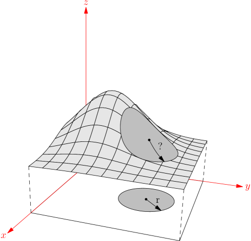
(a) Measuring distance in the $xy$-plane

(b) Measuring distance on the surface.

5.3: Distance measurement.

This simple example leads us to a more general conclusion: for distance measurement we can use any metric $g$. It is easy to verify that all the proofs remain valid if we change the Euclidean, often referred to as $L_{2}$ distance to another one. For example, we could use $L_{1}$ distance or, alternatively, the $L_{\infty}$ distance which is particularly suitable for computer simulations. Of course each choice of the metric changes the form of the robot’s effector. Three different forms, shown if Figures LABEL:fig:metrics_l2, LABEL:fig:metrics_l1, and LABEL:fig:metrics_linf correspond to $L_{1}$, $L_{2}$, and $L_{\infty}$ metrics accordingly.

(a) $L_{2}$ metric.

(b) $L_{1}$ metric.

(c) $L_{\infty}$ metric.

5.4: Use of different metrics.

Moreover we are not limited to 2-Dimensional spaces as the results remain valid for higher dimensions, e.g., we can use the same algorithm for covering 3D volumes assuming the robot’s effector is a ball of radius $r$ or, probably, a regular octahedron or a cube if we choose to work with $L_{1}$ or $L_{\infty}$ metrics respectively.

6 Simulations and Experiments

6.1 General Notes

We used $L_{\infty}$ metric in our experiments because the square shape of the effector and the sensing area that correspond to this metric is particularly suitable for computer simulations. In experiments with noise the robots were forced to start at non-noisy location, i.e., at locations with minimal pheromone level at time $t=0$. Additionally, in all experiments the robots were modeled as points and multiple robots were allowed to occupy the same location. We always measured the number of time steps until the robots covered the domain for the first time, averaged over 100 runs. Experiments were conducted on the domains shown in Figure LABEL:fig:domains.

(a) Domain A

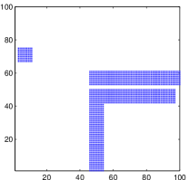
(b) Domain B

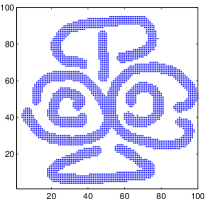
(c) Domain C

6.1: Simulation domains.

All domains are of size $100\times 100$ pixels and marking radius in all experiments was set to 3, i.e., each step robot marks a square of $5\times 5$ pixels. Figure LABEL:fig:maw-progress demonstrates some stages of covering Domain B by ten robots.

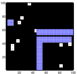
(a) Coverage: step 1

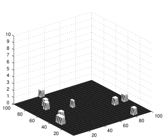
(b) Odor map: step 1

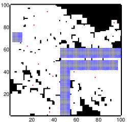
(c) Coverage: step 50

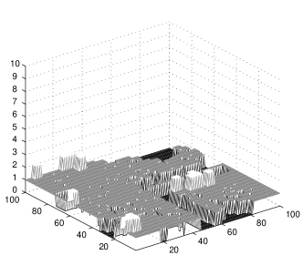
(d) Odor map: step 50

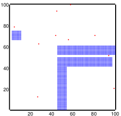
(e) Coverage: step 125

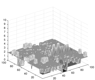
(f) Odor map: step 125

6.2: MAW progress on Domain B

6.2 Comparing MAW to other algorithms

In this experiment we studied performance of three different algorithm: MAW, MAC [Wagner et al. (2000)], and Random Walk. All algorithms used the same square effector of size $5\times 5$ pixels; additionally, the steps of the Random Walk algorithm were restricted to be in interval $[r,2r]$ just like the steps in the MAW algorithm.

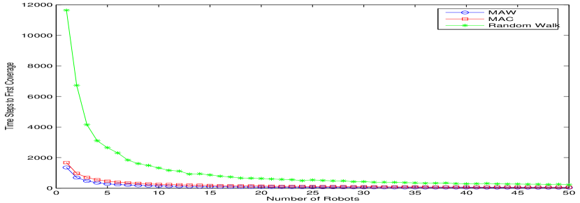
(a) Cover Time: Domain A

6.3: Cover Time

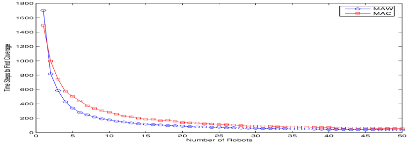
(b) Cover Time: Domain B

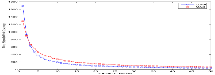
(c) Cover Time: Domain C

6.3: Cover Time

As we can see the MAW algorithm is a clear winner when we use three or more robots. For fewer robots the MAC algorithm performs better on complex domains. Note that the MAW algorithm in general performs better than the theoretical upper bound we got in Section LABEL:sec:maw-effic-analys. Cover time of the Random Walk was omitted from Figures LABEL:fig:cover-time-b and LABEL:fig:cover-time-c because the values were so big that the difference between the MAC and the MAW algorithms became invisible on this scale. Full results with additional statistical data can be seen in Appendix LABEL:sec:app_A.

Note that our upper bound on coverage time is quadratic, while the above results suggest that the actual coverage time is linear. We can demonstrate the predicted quadratic coverage time by tailoring specific tie breaking rules for specific domain. For example we can use a domain comprised of $n$ loops as shown in Figure LABEL:fig:loops_domain.

6.4: Domain comprised of $n$ loops

For this domain and specific tie breaking rules we can obtain quadratic coverage time for MAW algorithm, while MAC algorithm still demonstrates linear coverage time. These results are shown in Figure LABEL:fig:loops_results.

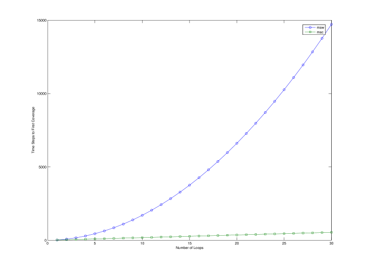
6.5: Worst case coverage time of specific domain

6.3 MAW in noisy environments

In this section we present the results of our simulation of MAW algorithm in presence of noise. In the first scenario we ran one robot on the Domain A, each time changing the amount of noisy pixels. Noise values are uniformly distributed in interval $[1,10]$, i.e., given that 60 percent of the pixels are noisy there are about 6 percent that got value of 1, 6 percent that got value of 2 and so on. Example of such noise profile with 60 percent noisy pixels is shown in Figure LABEL:fig:noise1.

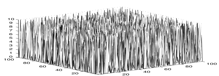
6.6: Example of noise profile 1.

In Figure LABEL:fig:noise-time we demonstrate the cover time as a function of the amount of noisy pixels in this scenario.

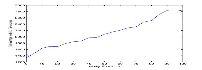
6.7: Cover time in noisy environment

In another scenario we chose to explore the influence of constant noise values on the performance of the algorithm. This time noise values in each experiment were constant and again randomly distributed in the space. Example of such noise profile for noise value of 10 and 30 percent noisy pixels is shown in Figure LABEL:fig:noise2.

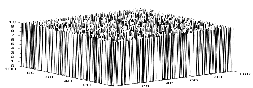
6.8: Example of noise profile 2.

We run a series of experiments with the noise values of 10, 20, 30, 40, and 50. The results of the cover time versus the percentage of noisy pixels is shown in Figure LABEL:fig:noise-time2.

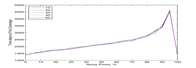
6.9: Cover time in noisy environment

As you can see the value of the noise does not play any role in this scenario, at least in the limits we used here, from 10 to 50. This is probably due to the nature of the algorithm that knows to discard high pheromone values in presence of lower values. To check this we conducted another experiment, that is similar to this one, however noise is this scenario occupies a compact space in the domain, i.e., given that there 40 percent of noisy pixels we form a plateau of noise as shown in Figure LABEL:fig:noise3

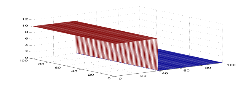
6.10: Example of noise profile 3.

In this case the influence of the noise value if pronounced as one can expect. See Figure LABEL:fig:noise-time3 for covering time versus noisy pixel percentage for noise values of 10, 20, 30, 40, and 50.

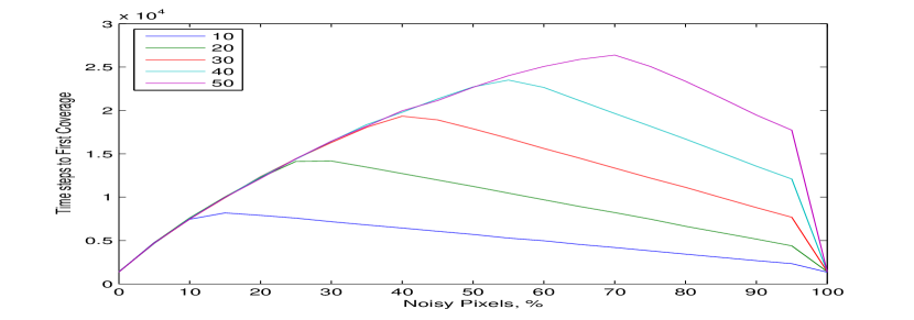
6.11: Cover time in noisy environment

As our experiments demonstrate the MAW algorithm has little sensitivity no “non-compact” distribution of the noise. Note that noise does not affect the Random Walk on the one hand and it destroys completely the MAC algorithm on the other hand, making it unable to cover the domain completely.

7 Conclusions

This work has two major contributions. First, we presented a new ant-inspired algorithm for continuous domain covering. We provided a formal proof of complete coverage and upper time bounds for complete coverage and the time interval between two successive visits of the robot. We also proved that the algorithm is immune to pheromone noise in the environment. A formal proof was provided for multi-robot coverage under the assumptions that the robots have different clock phases. Second, a new way of performance estimation was suggested, that implies some bounds on possible coverage time of any algorithm.

8 Detailed Statistics of MAW, MAC, and PC performance

8.1: MAW Results on Domain A

# robots	mean	max	min	std
1	1372.2	1999	1122	169.4
2	696.6	888	550	76.7
3	472.4	647	352	55.5
4	357.1	510	276	46.8
5	285.9	410	225	33.0
6	240.5	337	195	26.3
7	208.1	294	154	26.6
8	180.8	243	139	20.4
9	160.8	223	125	19.2
10	146.3	203	115	18.4
11	133.5	182	103	17.4
12	124.6	170	96	16.3
13	113.7	155	89	13.7
14	107.4	146	82	13.5
15	101.7	149	76	12.5
16	93.1	130	73	10.7
17	89.1	119	71	10.0
18	84.2	110	66	9.3
19	79.2	103	64	8.8
20	76.8	114	60	10.3
21	71.2	90	58	6.7
22	70.9	102	56	10.0
23	66.9	101	52	9.0
24	65.6	83	50	7.4
25	61.5	88	50	7.0
26	59.5	82	48	7.6
27	59.1	86	46	7.6
28	57.4	80	44	7.2
29	55.0	73	44	6.5
30	52.9	78	41	7.0
31	50.9	80	41	6.1
32	49.7	64	38	4.9
33	50.0	62	39	6.2
34	47.9	67	38	5.6
35	46.8	72	37	6.7

8.2: MAW Results on Domain B

# robots	mean	max	min	std
1	1689.6	3878	1021	500.8
2	830.5	1690	501	226.7
3	582.8	1411	365	193.9
4	454.6	1032	279	150.4
5	362.5	930	206	116.8
6	288.6	584	190	72.7
7	269.5	643	170	95.1
8	204.5	559	132	58.9
9	192.0	429	117	54.6
10	174.8	349	112	49.7
11	155.6	292	103	41.9
12	144.7	305	93	41.5
13	127.3	263	88	34.3
14	123.6	264	73	33.2
15	116.7	248	73	31.4
16	112.9	231	69	31.9
17	102.3	227	66	26.4
18	98.2	204	64	25.7
19	95.5	207	63	26.3
20	91.5	199	57	25.1
21	84.8	153	60	18.9
22	80.1	143	54	18.0
23	76.3	149	50	18.3
24	75.6	177	50	23.3
25	69.8	185	48	20.0
26	69.3	147	43	19.0
27	65.1	127	44	14.6
28	63.9	153	44	16.8
29	63.2	172	40	19.2
30	59.4	111	39	13.8
31	57.0	106	40	12.5
32	56.8	105	36	13.1
33	53.1	93	35	10.5
34	53.9	102	34	12.7
35	49.0	77	34	8.6

8.3: MAW Results on Domain C

# robots	mean	max	min	std
1	1713.3	4143	1076	579.0
2	881.0	2413	492	355.3
3	558.3	1176	342	149.5
4	444.7	1009	258	130.0
5	335.3	650	222	89.6
6	294.4	674	191	91.5
7	243.8	579	162	69.4
8	227.0	698	121	83.9
9	190.9	421	124	51.2
10	176.1	446	115	54.6
11	158.2	356	103	49.4
12	148.8	332	88	40.1
13	133.6	251	87	35.7
14	129.5	326	84	39.7
15	118.2	216	75	29.8
16	110.8	202	70	29.5
17	99.9	196	60	23.9
18	96.0	175	69	20.5
19	92.8	167	67	23.9
20	89.7	195	56	23.2
21	82.2	193	52	21.2
22	77.1	131	53	14.9
23	78.4	227	51	25.4
24	77.2	203	49	21.6
25	72.5	166	51	18.6
26	66.5	117	46	12.0
27	65.7	104	40	13.2
28	64.8	130	42	16.6
29	61.1	97	39	11.9
30	60.1	89	40	11.5
31	56.5	109	35	14.1
32	57.2	102	39	13.4
33	55.2	94	39	12.4
34	50.7	96	35	9.2
35	52.1	117	35	12.0

8.4: MAC Results on Domain A

# robots	mean	max	min	std
1	1679.7	1728	1586	26.9
2	966.1	1503	807	138.9
3	686.5	1078	540	99.1
4	565.2	885	423	92.2
5	451.6	734	318	67.9
6	386.3	710	300	67.8
7	347.9	551	244	66.0
8	302.7	655	222	55.5
9	275.1	444	196	53.4
10	260.0	495	184	53.8
11	234.8	439	167	47.8
12	214.8	338	154	37.6
13	198.3	276	144	30.8
14	188.9	304	131	39.4
15	179.2	282	123	34.9
16	166.7	286	110	35.6
17	159.9	244	110	26.7
18	148.7	237	107	27.6
19	142.0	226	95	26.7
20	140.6	322	90	34.7
21	135.8	299	86	35.2
22	126.3	226	87	24.0
23	119.6	195	86	22.2
24	117.8	206	76	27.0
25	114.0	202	76	26.5
26	105.1	148	69	18.8
27	103.8	190	72	19.2
28	104.3	170	70	22.2
29	95.5	139	69	15.4
30	95.0	182	63	20.1
31	94.6	170	65	18.3
32	89.8	155	61	20.2
33	88.0	181	61	18.5
34	81.4	125	53	14.7
35	80.0	135	50	15.7

8.5: MAC Results on Domain B

# robots	mean	max	min	std
1	1491.2	1540	1389	26.4
2	986.1	1344	723	172.4
3	729.4	1238	501	165.0
4	601.7	1090	374	150.3
5	479.9	807	300	117.3
6	410.6	716	266	92.1
7	377.4	723	223	108.7
8	352.6	719	206	106.2
9	304.2	630	168	94.8
10	290.7	558	171	89.4
11	262.3	525	147	86.1
12	238.2	485	127	74.9
13	225.8	500	128	76.0
14	208.2	440	115	67.1
15	201.2	414	114	69.1
16	173.3	412	91	52.7
17	163.1	373	96	48.8
18	163.1	390	100	55.9
19	147.5	274	92	43.4
20	146.6	367	86	50.2
21	133.1	338	85	46.0
22	125.0	332	84	35.5
23	123.1	372	77	37.6
24	118.1	243	70	31.6
25	121.7	322	71	42.8
26	104.0	218	63	28.2
27	103.4	209	66	26.1
28	95.3	164	68	21.2
29	96.8	322	64	32.7
30	94.3	186	61	24.5
31	88.0	164	59	21.2
32	89.6	257	56	26.7
33	81.5	195	56	21.0
34	80.2	144	48	17.4
35	79.0	146	54	17.4

8.6: MAC Results on Domain C

# robots	mean	max	min	std
1	1493.8	1559	1429	24.4
2	975.0	1361	752	175.0
3	705.2	1133	484	123.4
4	577.3	952	358	112.9
5	485.6	712	296	101.5
6	410.1	705	254	102.7
7	392.8	652	222	103.2
8	334.9	594	213	86.2
9	294.7	707	181	90.0
10	274.3	558	144	75.6
11	261.5	548	151	87.1
12	229.6	481	145	65.5
13	226.2	473	125	73.6
14	200.2	512	119	61.6
15	185.9	375	108	56.3
16	165.9	361	111	45.5
17	164.9	428	95	53.8
18	160.8	380	84	53.6
19	146.3	311	94	42.7
20	144.4	290	86	40.1
21	132.6	320	85	39.0
22	127.6	262	70	35.2
23	118.1	390	75	39.5
24	114.4	218	77	29.8
25	110.1	288	74	36.5
26	108.9	240	65	31.5
27	103.6	258	67	32.7
28	100.4	193	65	26.6
29	96.2	171	64	23.7
30	94.7	176	59	22.7
31	91.5	170	59	21.6
32	86.7	178	59	22.8
33	84.2	188	55	22.1
34	81.9	170	52	18.9
35	79.5	173	55	19.6