Synchrotron signature of a relativistic blast wave with decaying microturbulence

Abstract

Microphysics of weakly magnetized relativistic collisionless shock waves, corroborated by recent high performance numerical simulations, indicate the presence of a microturbulent layer of large magnetic field strength behind the shock front, which must decay beyond some hundreds of skin depths. The present paper discusses the dynamics of such microturbulence, borrowing from these same numerical simulations, and calculates the synchrotron signature of a powerlaw of shock accelerated particles. The decaying microturbulent layer is found to leave distinct signatures in the spectro-temporal evolution of the spectrum $F_{\nu}\propto t^{-\alpha}\nu^{-\beta}$ of a decelerating blast wave, which are potentially visible in early multi-wavelength follow-up observations of gamma-ray bursts. This paper also discusses the influence of the evolving microturbulence on the acceleration process, with particular emphasis on the maximal energy of synchrotron afterglow photons, which falls in the GeV range for standard gamma-ray burst parameters. Finally, this paper argues that the evolving microturbulence plays a key role in shaping the spectra of recently observed gamma-ray bursts with extended GeV emission, such as GRB090510.

1 Introduction

The acceleration of particles at a decelerating relativistic collisionless shock front constitutes a key building block of the afterglow model of gamma-ray bursts (GRB, Mészáros & Rees 1997). The standard phenomenology models the accelerated electron population as powerlaw ${\rm d}N_{e}/{\rm d}\gamma_{e}\propto\gamma_{e}^{-p}$, which radiates powerlaw photon spectra of the form $F_{\nu}\propto t^{-\alpha}\nu^{-\beta}$, with a temporal decay index $\alpha$ and a frequency index $\beta$ that are direct functions of $p$, see e.g. Piran (2005) for a review, or e.g. Sari et al. (1998), Panaitescu & Kumar (2000) for detailed formulae. From both microscopic and observational points of view, the situation however appears more complex, in spite of several remarkable results of the past decade.

On the microscopic level, for instance, one understands the formation of a relativistic collisionless shock front in a weakly magnetized medium – such as the interstellar medium (ISM) – through the self-generation of intense small scale electromagnetic fields that act as the mediating agents for the transition from the far upstream unshocked state to the far downstream shocked state. The accelerated particles, as forerunners of the shock front, play a central role in triggering the microinstabilities that build the self-generated field. In turn, this self-generated microturbulence controls the scattering of these particles and it therefore directs the acceleration process, which becomes intricately non-linear. This general scheme has been validated so far in high performance particle-in-cell (PIC) simulations (e.g. Spitkovsky 2008, Keshet et al. 2009, Sironi & Spitkovsky 2009, 2011, Martins et al. 2009) and understood on the basis of analytical arguments at the linear level (e.g. Medvedev & Loeb 1999, Gruzinov & Waxman 1999, Lyubarsky & Eichler 2006, Lemoine & Pelletier 2010, 2011a, Rabinak et al. 2011). The situation becomes more complex when one tries to bridge the gap between the limited simulation timescales and the much longer timescales probed by the observations. On such timescales, one would indeed expect that the microturbulence has died away (e.g. Gruzinov & Waxman 1999), yet GRB afterglow modelling has generally pointed to a field strength close to a percent of equipartition permeating the blast, on day timescales. The origin of this field and its relation with the microturbulence behind the shock front has remained a nagging issue for many years.

On the observational level, the recent era of rapid follow-up observations in the X-ray and GeV domain has brought its wealth of surprises. The Swift satellite has revealed X-ray afterglow light curves that differ appreciably in the $10^{2}-10^{4}\,$s domain from the canonical afterglow model (Nousek et al. 2006, O’Brien et al. 2006). Of more direct interest to the present work, the Fermi-LAT telescope has reported the discovery of long-lived ($\sim 100-1000\,$s) GeV emission in a fraction of observed bursts. In one case (GRB090510), this emission has been measured almost contemporarily to emission in the X-ray and optical domains as early as $100\,$s (Ackermann et al. 2010, de Pasquale et al. 2010). This long-lived high energy emission has been shown to fit nicely the predictions of a model in which the electrons cool slowly through synchrotron radiation in a background shock compressed magnetic field, without any need for microturbulence (Barniol-Duran & Kumar 2009, 2010, 2011a; see also Gao et al. 2009; de Pasquale et al. 2010; Corsi et al. 2010; Ghirlanda et al., 2010; He et al 2011; and see Ghisellini et al. 2010, Razzaque 2010 and Panaitescu 2011 for alternative points of view). Given the past history in GRB afterglow modelling, such a low magnetization of the blast may come as a surprise, but it may also point out that after all, the microturbulence does decay away as theoretically expected, and that the high level of turbulence seen on day timescales has been seeded through some other instability.

Depending on how fast and how far from the shock this microturbulent layer decays, it is likely to influence the particle energy gains from Fermi acceleration, and losses through synchrotron radiation. The microturbulent layer must actually ensure the scattering of accelerated particles, because in the absence of microturbulence, these particles would be advected away with the transverse magnetic field lines to which they are tied and acceleration would not take place (e.g. Begelman & Kirk 1990, Lemoine et al. 2006, Niemiec et al. 2006, Pelletier et al. 2009). Now, scattering in small scale turbulence is so slow that producing GeV photons at an external blast wave of Lorentz factor of a few hundreds represents a challenge, see e.g. Kirk & Reville (2010), Lemoine & Pelletier (2011c), and see also Piran & Nakar (2010), Sagi & Nakar (2012). It would be about impossible if the particles were to scatter in the microturbulent layer then radiate in the much weaker shock compressed background field. Therefore, the interpretation of Barniol-Duran & Kumar (2009, 2010, 2011a) actually suggests that the microturbulence also plays a role in the radiation of GeV photons, at the very least, if not in shaping the synchrotron spectra over the broad spectral range. In other words, the observation of extended GeV emission and its early follow-up in other wavebands may be opening a rare window on the dynamics of the microturbulence in weakly magnetized relativistic collisionless shocks.

In this context, the present paper proposes to discuss the synchrotron spectra and more generally the afterglow spectrum $F_{\nu}\propto t^{\-\alpha}\nu^{-\beta}$ of a decelerating relativistic blast wave, accounting for the time evolution of the microturbulence behind the shock front. While the initial motivation of this work was to provide a concrete basis for the scenario of Barniol-Duran & Kumar (2009, 2010, 2011a), in which particles scatter in a time decaying microturbulence but radiate in a region devoid of microturbulence, it has become apparent that the possibility of decaying microturbulence opens a quite rich diversity of phenomena, which deserve to be discussed in detail. This problem has been tackled by Rossi & Rees (2003), who considered the simplified case of a homogeneous microturbulent layer that dies instantaneously beyond some distance, and by Derishev (2007), who showed that a particle radiating in a time evolving magnetic field can lead to spectra quite different from the standard one-particle synchrotron spectra. Borrowing from the latest PIC simulations, the present paper establishes a model of the microturbulence strength and coherence length evolving as powerlaws in time beyond some distance, until the decay saturates down to the background shock compressed magnetic field; the present study then calculates the synchrotron spectra in this structure for various typical configurations (slow cooling, fast cooling, with and without inverse Compton losses) and it discusses the problem of particle scattering, acceleration timescale and maximum photon energy in this setting. As such, it generalizes and encompasses these former studies, in the spirit of providing new tools with which one can analyse existing and forthcoming data. A brief comparison to present early afterglow observations is provided.

The detailed spectra and the spectro-temporal indices $\alpha$, $\beta$ of $F_{\nu}\,\propto\,t^{-\alpha}\nu^{-\beta}$ are provided in Appendix A, while Section 2 details the model for the evolution of microturbulence and provides the general characteristics of the afterglow light curves and spectral energy distributions in various configurations. Section 3 discusses the scattering process and the maximal acceleration energy, and it confronts the above models to existing data. The results are summarized in Sec. 4. Throughout, this paper adopts the standard notation $Q_{x}\equiv Q/10^{x}$ with $Q$ a generic quantity in cgs units. Fiducial values used for numerical applications correspond to those derived in Barniol-Duran & Kumar (2009, 2010, 2011a), and He et al. (2011), e.g. an external density $n\sim 10^{-3}\,$cm^-3, a blast Lorentz factor $\gamma_{\rm b}\sim 300$ at $100\,$s and it is assumed that the blast has entered the deceleration regime. One must distinguish the time $t_{\rm obs}$ in the observer frame, also written $t_{\rm obs}=100\,t_{2}\,$s in numerical applications, from the time experienced by a particle since shock entry; this difference is manifest everywhere. For convenience, the notation $z_{+,0.3}\,\equiv\,(1+z)/2$ is introduced, $z$ denoting the redshift of the GRB.

2 Synchrotron spectra with time decaying microturbulence

The self-generation of microturbulence in the precursor of a relativistic collisionless shock front propagating in a very weakly magnetized medium appears both guaranteed and necessary to the maintenance of the shock. It is necessary because in the absence of a background magnetic field, self-magnetization is required to build up a magnetic barrier that initiates the shock transition. It is guaranteed because the development of microinstabilities follows naturally from the penetration of the unshocked plasma by the anisotropic beam of supra-thermal particles moving ahead of the shock (e.g. Medvedev & Loeb 1999).

Studies of non-relativistic collisionless magnetospheric shocks have shown that dissipation ahead of the shock is initiated by the reflection of ambient particles (i.e. from the unshocked plasma) on the shock front in the compressed magnetic field (e.g. Leroy et al. 1982). Particle-in-cell simulations indicate that a similar phenomenon takes place at a relativistic unmagnetized shock, although the particles now reflect on the small scale electromagnetic fields self-generated by the microinstabilities (e.g. Spitkovsky 2008). The reflected and accelerated particle populations merge together and trigger microinstabilities such as the Weibel (filamentation) instability or oblique electrostatic instabilities, provided the precursor extends far enough for these modes to grow on the precursor crossing timescale (Lemoine & Pelletier 2010, 2011a). In a very weakly magnetized shock wave, with magnetization typical of the ISM and blast Lorentz factor $\gamma_{\rm b}\lesssim 10^{3}$, this appears guaranteed.

As seen from the shock frame (in which the shock front lies at rest) the incoming kinetic energy is carried by the protons, the electrons carrying only a fraction $m_{e}/m_{p}$ of the incoming flow kinetic energy. Energy transfer between the two species in the microturbulence leads to heating of the electron population, close to equipartition by the time it reaches the shock front, as observed in current PIC simulations (Sironi & Spitkovsky 2011), see also the discussion in Lemoine & Pelletier (2011a). Equipartition means that the incoming electrons carry Lorentz factor $\gamma_{e}\sim\gamma_{\rm b}m_{p}/m_{e}$, hence their skin depth scale (downstream frame) $c/\left[4\pi\gamma_{\rm b}n_{\rm u}/\left(\gamma_{e}m_{e}\right)\right]^{1/2}\sim c/\omega_{\rm pi}$. The natural length scale of the electromagnetic structures produced by these microinstabilities is therefore the ion skin depth scale $c/\omega_{\rm pi}$ of the upstream plasma.

2.1 Input from Particle-in-cell simulations

Particle-in-cell simulations not only validate the above general scheme, they also provide interesting constraints on the shape and evolution of microturbulence ahead and behind the shock front. Two most recent and most detailed studies are of direct interest to the present work.

Chang et al. (2008) have performed long simulations of the evolution of micro-turbulence behind a relativistic shock front. The simulations have been computed for an unmagnetized pair plasma with relative Lorentz factor $\gamma_{\rm b}=15$ between upstream and downstream. In weakly magnetized relativistic shock waves, the preheating of electrons in an electron-ion shock of similar configuration appears so efficient that for all practical matters, the downstream plasma behaves as a relativistic pair plasma; hence the results of Chang et al. (2008) can be transposed to an electron-ion shock. These simulations show that the microturbulence remains mostly static in the downstream rest frame, and that it is composed of an intermittent magnetic field structure that can be roughly described as a collection of magnetic loops and islands on typical length scales $\sim 10-30\,c/\omega_{\rm pi}$. One clear observation made in this work is that the small scale structures dissipate first, leaving the large scale clumps unaffected over the timescale of the simulation. Chang et al. (2008) interpret this gradual erosion as collisionless damping, with a damping frequency $\Im\omega\propto\lambda^{-3}$ ($\lambda$ denoting the spatial scale). If the magnetic turbulence is described in Fourier space as a power law spectrum with most of magnetic power on small length scales, this implies a decay of the magnetic field strength accompanied by an evolution of the coherence scale $\lambda_{\delta B}\propto t^{1/3}$. This is made explicit further below.

The longest PIC simulation so far for a relativistic shock is that of Keshet et al. (2009), which extends to about $10^{4}\omega_{\rm pi}^{-1}\,\sim\,240\,n_{-3}^{-1/2}\,$s (comoving time). For values envisaged by Barniol-Duran & Kumar (2009, 2010, 2011a) and He et al. (2011) to describe the GeV extended emission, i.e. an ejecta of energy $E\sim 10^{53}\,$erg, launched into a medium of density $n\sim 10^{-3}\,$cm^-3 with initial Lorentz factor $\gamma_{\rm ej}\sim 10^{3}$, the above timescale represents close to $1\,$% of a dynamical timescale at an observer time of a hundred seconds. Keshet et al. (2009) provide a detailed study of the magnetic field power spectrum of the turbulence and its evolution. They confirm most of the findings of Chang et al. (2008); in particular, they show that the magnetic field does decay behind the shock wave, but on rather long length scales compared to a skin depth $c/\omega_{\rm pi}$. More importantly, they find that the presence of shock accelerated particles influences the decay timescale of the magnetic field with a general trend being that higher energy particles ensure a longer lifetime for the downstream microturbulence. Given that the simulations of Keshet et al. (2009) extend for a time that is much smaller than the dynamical time, it has not had time to produce very high energy particles and to probe their impact. Such high energy particles would tend to populate the magnetic perturbation spectrum with longer wavelength modes, which would then decay on longer timescales when downstream. In any event, this should not call into question what has been said above, since low energy particles carry most of the energy of a shock accelerated population with index $p>2$. Nevertheless, to probe how far the perturbation spectrum may be populated, one can conduct the following exercise. The maximal size of the precursor is given in a reasonable approximation by $r_{{\rm L,max},i,0}/\gamma_{\rm sh}^{3}$, where $r_{{\rm L,max},i,0}$ represents the gyration radius of the highest energy ions in the background upstream magnetic field, and $\gamma_{\rm sh}=\sqrt{2}\gamma_{\rm b}$ the shock Lorentz factor as measured upstream. This result is discussed in detail in Plotnikov et al. (2012) but it can be understood as follows. The highest energy ions are those that travel the furthest away from the shock, since electrons are generally accelerated to a smaller energy due to synchrotron losses; furthermore, the particles gyrate by an angle $1/\gamma_{\rm sh}$ over a timescale $t_{\rm res,u}\simeq c^{-1}r_{{\rm L,max},i,0}/\gamma_{\rm sh}$ before being caught up by the shock front (Achterberg et al. 2001); finally, the typical distance between the shock front and the particle is $c\,t_{\rm res,u}\left(1-\beta_{\rm sh}\right)\sim c\,t_{\rm res,u}/(2\gamma_{\rm sh}^{2})$. Assuming that the ions are accelerated on a timescale $t_{\rm res,u}$ (see also Sec. 3.1) and comparing the time available for acceleration with the age of the shock wave $r/c$, one finds the precursor size $\sim r/\gamma_{\rm sh}^{2}\sim 2\times 10^{4}\left(c/\omega_{\rm pi}\right)n_{-3}^{1/2}t_{2}z_{+,0.3}^{-1}$. This indicates that the perturbation may well extend on several decades. In the absence of ions, the precursor size would be set by the highest energy electrons; balancing acceleration at a Bohm rate (as experienced downstream) to synchrotron losses, one would find a precursor size about 20 times smaller for the adopted fiducial parameters, nevertheless much larger than the typical size of the fluctuations.

Finally, Keshet et al. (2009) suggest a damping frequency $\Im\omega\propto\lambda^{-2}$, which implies, when combined with the above result that the decay of the microturbulence might extend over quite long spatial scales.

Following Chang et al. (2008), the magnetic field power spectrum is described as a time decaying powerlaw form in the downstream (comoving) frame, with

$$\langle\delta B(t)^{2}\rangle\,=\,a_{B}\,\delta B_{\mu}^{2}\,\int_{\lambda_{\mu}}^{\lambda_{\rm max}}\frac{{\rm d}\lambda}{\lambda_{\mu}}\left(\frac{\lambda}{\lambda_{\mu}}\right)^{\alpha_{B}}\exp\left(-\frac{t}{\tau_{\lambda}}\right)\ ,$$ (1)

with $t$ denoting the time (downstream frame) since shock entry of the corresponding plasma element, $\lambda_{\mu}$ (resp. $\lambda_{\rm max}$) the minimum (resp. maximum) wavelength scale of the microturbulence at $t=0$, $\alpha_{B}<-1$ so that the turbulent power lies at the smallest scales, $a_{B}\,\equiv\,|1+\alpha_{B}|$ for normalization purposes, $\delta B_{\mu}$ denotes the rms field strength at $t=0$ and $\tau_{\lambda}=\left|\Im\omega\right|^{-1}$ the damping time, which depends on $\lambda$:

$$\tau_{\lambda}\,\equiv\,\omega_{\rm pi}^{-1}\left(\omega_{\rm pi}\lambda/c\right)^{\alpha_{\lambda}}\ .$$ (2)

Assuming $\lambda_{\rm max}\gg\lambda_{\mu}$ for the moment, Eq. (1) can be integrated in terms of an incomplete Gamma function,

$$\langle\delta B(t)^{2}\rangle \,=\, \delta B_{\mu}^{2}\,\alpha_{\lambda}^{-1}\mu(t)^{(1+\alpha_{B})/\alpha_{\lambda}}$$

$$\,\,\times\left\{\Gamma\left(-\frac{1+\alpha_{B}}{\alpha_{\lambda}}\right)-\Gamma\left[-\frac{1+\alpha_{B}}{\alpha_{\lambda}};\,\mu(t)\right]\right\}\ ,$$

with

$$\mu(t)\,\equiv\,\omega_{\rm pi}\,t\,\left(\frac{\omega_{\rm pi}\lambda_{\mu}}{c}\right)^{-\alpha_{\lambda}}\ .$$ (4)

For convenience, one may approximate Eq. (LABEL:eq:dbt) with respectively the small and large argument limits to describe the evolution of the magnetic field strength as

$$\langle\delta B(t)^{2}\rangle\,\simeq\,\begin{cases}\delta B_{\mu}^{2}&\text{if}\,\,\mu(t)<1\ ,\\ \delta B_{\mu}^{2}\Gamma\left(1+|\alpha_{t}|\right)\mu(t)^{\alpha_{t}}&\text{if}\,\,\mu(t)\gg 1\ ,\end{cases}$$ (5)

with the following definition

$$\alpha_{t}\,\equiv\,\frac{1+\alpha_{B}}{\alpha_{\lambda}}\,<0\ .$$ (6)

In the following, the numerical factor $\Gamma\left(1+|\alpha_{t}|\right)$, of order unity, will be dropped henceforth.

Equation 6 shows that the temporal decay index of the magnetic field behind the shock is inherently linked to how power is distributed on scales larger than the minimum scale $\lambda_{\mu}$ – as characterized by $\alpha_{B}$ – and to how fast small scale features are dissipated – as characterized by $\alpha_{\lambda}$. The interpretation for this is clear: as small scales are erased, magnetic power is removed, but the rate at which the total strength erodes depends on how much strength is left at longer wavelengths. In fine, the uncertainty on $\alpha_{t}$ is related to the sourcing of large wavelength fluctuations, which are likely related to the dynamics of high energy particles in the upstream. The above assumption $\lambda_{\rm max}\gg\lambda_{\mu}$ has been discussed above. Its robustness depends crucially on the influence of maximal energy particles upstream of the shock front. In the extreme opposite case $\lambda_{\rm max}\sim\lambda_{\mu}$, one should observe a roughly constant magnetic field while $\mu(t)<1$, followed by fast decay once $\mu(t)>1$. This situation may be accounted for by Eq. 5 with a more pronounced value of $\alpha_{t}$.

The following therefore considers a range of possibilities for $\alpha_{t}$, even though the PIC simulations of Chang et al. (2008) and Keshet et al. (2009) both suggest $-1<\alpha_{t}<0$. More specifically, Chang et al. (2008) suggest that the magnetic field Fourier spectrum (for $\delta B$, not $\delta B^{2}$) in wavenumber has slope $\simeq 0\rightarrow 1/2$, which corresponds to $1+\alpha_{B}\sim-2\rightarrow-1$, and $\alpha_{\lambda}=3$ leading to $\alpha_{t}\sim-1/3\rightarrow-2/3$. Keshet et al. (2009) show that right behind the shock front, the magnetic field decays exponentially on short a distance scale to level off at a strength corresponding to $\epsilon_{B}\sim 10^{-2}$ for some hundreds of skin depth. A closer inspection of their Fig.3 however reveals that the initial exponential decay leaves way to a powerlaw decay at late simulation times (thus meaning far downstream) and by eye, one estimates $\alpha_{t}\sim-0.5$. These simulations thus indicate a value of $\alpha_{t}$ between $-1$ and $0$; however, given the present limitations of the PIC simulations, and the above possible caveat related to the extension of the magnetic perturbation spectrum, one cannot exclude yet that $\alpha_{t}<-1$. In this respect, one must point out that recent simulations of the development and the dynamics of relativistic Weibel turbulence indeed suggest a value $\alpha_{t}\simeq-2$ (Medvedev et al. 2010). Although these simulations do not simulate the shock itself, but a Weibel turbulence through the interpenetration of two relativistic beams, these are 3D while the shock simulations of Chang et al. (2008) and Keshet et al. (2009) are 2D.

In order to account for these different possibilities in the following, Eq. 5 is kept in its present form, but the decay exponent $\alpha_{t}$ is assumed to take possibly mild or more pronounced values. Depending on whether $\alpha_{t}<-1$ or $-1<\alpha_{t}<0$, it will be seen that radically different radiative signatures are to be expected.

In summary, theoretical arguments combined with recent high performance PIC simulations suggest the following characterization for the evolution of the microturbulence behind a relativistic (weakly magnetized) shock front. Immediately behind the shock, the magnetic field carries strength $\delta B_{\mu}$ corresponding to an equipartition parameter $\epsilon_{B}\equiv\delta B_{\mu}^{2}/\left(32\pi\gamma_{\rm b}^{2}nm_{p}c^{2}\right)$ with fiducial value $\epsilon_{B}\sim 10^{-2}$, while $\lambda_{\mu}\sim 10-30c/\omega_{\rm pi}$ represents the fiducial value for the coherence scale at that same location. The magnetic field strength decays as $t^{\alpha_{t}}$ after a time

$$t_{\mu+}\,\equiv\,\omega_{\rm pi}^{-1}\left(\omega_{\rm pi}\lambda_{\mu}/c\right)^{\alpha_{\lambda}}\ ,$$ (7)

defined through $\mu(t_{\mu+})\,\equiv\,1$, of the order of hundreds to thousands of inverse plasma times, until it eventually settles at the shock compressed value $B_{\rm d}=4\gamma_{\rm b}B_{\rm u}$. In the following, this timescale is rewritten in units of inverse plasma times as

$$\Delta_{\mu}\,\equiv\,\omega_{\rm pi}t_{\mu+}\ ,$$ (8)

meaning also that the undecayed part of the microturbulence extends for $\Delta_{\mu}$ skin depths. Note that $\Delta_{\mu}\,\gg\,1$ according to the above simulations. Finally, the coherence length of the microturbulence evolves as $t^{1/\alpha_{\lambda}}$, with fiducial value $\alpha_{\lambda}\sim 2-3$.

2.2 Radiation in time decaying microturbulence

As a particle gets Fermi accelerated, it interacts with the turbulent layer within a scattering length scale $l_{\rm scatt}$ of the shock front. This scattering length scale controls the residence time hence the acceleration timescale hence the maximal energy that can be reached; it is discussed in more detail in Sec. 3.1. For the time being, it suffices to note that the Larmor radius of the bulk of the electrons, with minimum Lorentz factor $\gamma_{\rm m}=|p-1|^{-1}|p-2|\epsilon_{e}\gamma_{\rm bl}m_{p}/m_{e}$ is so small that these electrons can only explore the undecayed part of the turbulence:

$$r_{\rm L}\left(\gamma_{\rm m}\right)\,\approx\,\epsilon_{e,-0.3}\epsilon_{B,-2}^{-1/2}\frac{c}{\omega_{\rm pi}}\,\ll\,\lambda_{\mu}\ .$$ (9)

The microturbulence thus controls the acceleration of the bulk of electrons, independently of how fast this microturbulence decays or how large the blast Lorentz factor may be. At Lorentz factors $\gg\gamma_{\rm m}$ of interest for high energy radiation, the electrons may start to explore the region $\mu(t)>1$. Then the transport becomes non trivial; its impact on acceleration is discussed in Sec. 3.1.

During the acceleration stage, the particle moves in a near ballistic manner and diffusive effects can be neglected, given that the return probability decreases fast with the number of steps of length $l_{\rm scatt}$ taken. Therefore, as a particle moves away from the shock on a distance scale $x$ along the shock normal during a time $t_{\rm p}\sim x/(c\cos\theta)$, with $\theta$ the angle to the shock normal, it explores a microturbulence that has decayed according to the laws given above with $t\simeq 3\cos\theta\,t_{\rm p}$. This factor of $3$ of course results from the convective velocity $c/3$ of the downstream plasma.

On length scales much larger than $l_{\rm scatt}$, a particle diffuses in the microturbulence and in a first approximation, one can describe its transport by advection with the downstream plasma. For such particles, $t\simeq t_{\rm p}$. The above slight difference between $t$ and $t_{\rm p}$ does not impact the results given further below and can be neglected in view of the uncertainties related to the time evolution of the turbulence. In the following, $t$ and $t_{\rm p}$ are thus be used interchangeably.

The cooling history of an electron of Lorentz factor $\gamma_{e}$ obeys the standard law

$$\frac{{\rm d}\gamma_{e}}{{\rm d}t}\,=\,-\frac{1}{6\pi}\sigma_{\rm T}\frac{\delta B(t)^{2}(1+Y)}{m_{e}c}\gamma_{e}^{2}\ ,$$ (10)

with $Y$ the Compton cooling factor. For the time being, one considers the simple case $Y\ll 1$; the influence of inverse Compton losses is discussed in detail in App. A and further below. One then defines a Lorentz factor $\gamma_{\mu+}$ such that, if $\gamma_{e}>\gamma_{\mu+}$, the particle cools in the undecayed microturbulence where $\mu(t)<1$ (at time $t<t_{\mu+}$), while if $\gamma_{e}<\gamma_{\mu+}$, the particle does not cool in that layer but further on. Writing the synchrotron cooling time for particles of Lorentz factor $\gamma_{e}$ in a (constant) magnetic field of strength $\delta B$ as $t_{\rm syn}\left[\gamma_{e};\delta B\right]$, the Lorentz factor $\gamma_{\mu+}$ can also be defined as the solution of

$$\gamma_{\mu+}:\quad\mu\left[t_{\rm syn}\left(\gamma_{\mu+};\delta B_{\mu}\right)\right]\equiv 1\ .$$ (11)

In terms of the fiducial values of interest here,

$$\gamma_{\mu+}\,\simeq\,3\times 10^{9}\,t_{2}^{3/4}E_{53}^{-1/4}n_{-3}^{-1/4}\epsilon_{B,-2}^{-1}\Delta_{\mu,2}^{-1}\ ,$$ (12)

with $\Delta_{\mu,2}=\Delta_{\mu}/100$. This value of $\gamma_{\mu+}$ generally exceeds the maximal Lorentz factors that can be achieved through shock acceleration, therefore particles cool outside this undecayed turbulent layer, unless $\Delta_{\mu}$ is larger than expected, as discussed in Sec. 3.1. The latter may well happen, if for instance $\alpha_{\lambda}>2$ and/or $\lambda_{\mu}\gg 10c/\omega_{\rm pi}$.

If a particle exits the acceleration process with a Lorentz factor $\gamma_{e,0}$, then at time $t$,

$$\gamma_{e}\,\simeq\,\begin{cases}\displaystyle{\frac{\gamma_{e,0}}{1+\gamma_{e,0}/\gamma_{\mu+}}}&(\mu(t)\ll 1)\\ \displaystyle{\frac{\gamma_{e,0}}{1+(1+\alpha_{t})^{-1}\left[\mu(t)^{1+\alpha_{t}}+\alpha_{t}\right]\gamma_{e,0}/\gamma_{\mu+}}}&(\mu(t)\gg 1)\ .\end{cases}$$ (13)

If $\gamma_{e0}>\gamma_{\mu+}$, the particle cools down to $\gamma_{\mu+}$ within the layer where $\mu(t)<1$ (i.e. $t<t_{\mu+}$) and subsequently, it continues cooling if $-1<\alpha_{t}<0$ or stops its cooling if $\alpha_{t}<-1$. If $\gamma_{e0}<\gamma_{\mu+}$ on the contrary, the particle either cools later in the decaying microturbulence if $-1<\alpha_{t}<0$, or not if $\alpha_{t}<-1$. In any case, the particle of course eventually cools in the background shock compressed field (notwithstanding issues related to the available hydrodynamical timescale). Whichever occurs influences the afterglow light curve and spectral energy distribution.

If $-1<\alpha_{t}<0$, it is convenient to define a second Lorentz factor, $\gamma_{\mu-}$, as the Lorentz factor for which cooling occurs on a timescale $t_{\mu-}$ such that $\delta B\left(t_{\mu-}\right)=B_{\rm d}$, i.e. at the time at which the turbulence field has relaxed to the background shock compressed value $B_{\rm d}=4\gamma_{\rm bl}B_{\rm u}$. For the time being, no consideration is made of the hydrodynamical timescale of the blast. Then, if $\gamma_{\rm m}>\gamma_{\mu-}$ (and $\alpha_{t}>-1$), most particles cool in the decaying microturbulent layer. One finds

$$\frac{\gamma_{\mu-}}{\gamma_{\mu+}}\,\simeq\,\left(\frac{\sigma_{\rm u}}{\epsilon_{B}}\right)^{-(1+\alpha_{t})/\alpha_{t}}\ ,$$ (14)

in terms of the upstream magnetization parameter $\sigma_{\rm u}\,\equiv\,B_{\rm u}^{2}/(4\pi nm_{p}c^{2})$. The Lorentz factor $\gamma_{\mu-}$ depends exponentially on $\alpha_{t}$; it may therefore take very different values.

To calculate the radiative signature, one integrates over the cooling history of the electron population, as in Gruzinov & Waxman (1999), although for simplicity, the calculation is done in a one-dimensional quasi-steady state approximation, meaning that the secular hydrodynamical evolution of the blast is neglected in the course of this integration over the blast width. This method corresponds to the steady state approximation of Sari et al. (1998), when calculating the stationary electron distribution in a homogeneous shell. The spectral power density of the blast can then be written in the downstream frame in terms of an integral over a particle history, up to a (comoving) hydrodynamical timescale $t_{\rm dyn}$ (see Eq. 42)

$$P^{\prime}_{\nu}\,=\,\int_{\gamma_{\rm m}}^{\gamma_{\rm max}}\,\frac{{\rm d}\dot{N}_{e}}{{\rm d}\gamma_{e,0}}\,{\rm d}\gamma_{e,0}\,\,\int_{0}^{t_{\rm dyn}}{\rm d}t\,\frac{{\rm d}E_{\rm syn}(\gamma_{e,0})}{{\rm d}\nu{\rm d}t}\ ,$$ (15)

with ${\rm d}E_{\rm syn}/{\rm d}\nu{\rm d}t$ the spectral power density radiated by an electron at time $t$, of initial Lorentz factor $\gamma_{e,0}$ and of cooling history given by Eq. (13); see also Eq. 40. The above expression is folded over the injection distribution ${\rm d}\dot{N}_{e}/{\rm d}\gamma_{e,0}$, which is assumed to take a power law form between $\gamma_{\rm m}$ and $\gamma_{\rm max}\gg\gamma_{\rm m}$:

$${\rm d}\dot{N}_{e}\,=\,\dot{N}_{e}\,\frac{|1-p|}{\gamma_{\rm m}}\left(\frac{\gamma_{e,0}}{\gamma_{\rm m}}\right)^{-p}\,{\rm d}\gamma_{e,0}\ ,$$ (16)

with

$$\dot{N}_{e}\,=\,\gamma_{\rm b}\left(\beta_{\rm b}+\frac{1}{3}\right)4\pi nr^{2}c$$ (17)

the number of electrons swept and shock accelerated by the shock wave per unit time, as measured in the downstream frame.

The detailed calculation of the spectral power $P_{\nu}$ is carried out in Appendix A for different relevant cases. In particular, two distinctions have to be made: whether the microturbulence decays rapidly beyond $t_{\mu+}$ or not and whether inverse Compton losses contribute significantly to the cooling of electrons. These cases are examined in turn in the next subsections, in parallel to the discussion of App. A.

2.3 Gradual decay, no inverse Compton losses

As discussed in App. A, the gradual evolution of the microturbulence behind the shock affects the spectro-temporal flux $F_{\nu}$ in various ways. For one, particles of different Lorentz factors cool in different magnetic fields, with particles of lower energy experiencing lower magnetic fields at cooling. This implies that the characteristic synchrotron frequencies are modified and more specifically, that ratios of characteristic frequencies are stretched with respect to the standard case of a homogeneous turbulent layer. Regarding the cooling frequency $\nu_{\rm c}$, the modification is non-trivial because the cooling Lorentz factor $\gamma_{\rm c}$ itself depends in a non-trivial way on the temporal decay index of the turbulence, see Eq. 53. The characteristic frequency $\nu_{\rm m}$ associated to particles of Lorentz $\gamma_{\rm m}$ can also be modified in a non-trivial way, since $\nu_{\rm m}\,=\,\nu_{\rm p}\left[\gamma_{\rm m};\delta B_{\gamma_{\rm m}}\right]$, with $\nu_{\rm p}$ defined as the synchrotron peak frequency of particles of Lorentz factor $\gamma_{\rm m}$ in a magnetic field of strength $\delta B_{\gamma_{\rm m}}$, see Eq. 45. The magnetic field $\delta B_{\gamma_{\rm m}}$ in which the particles of Lorentz factor $\gamma_{\rm m}$ radiate most of their energy takes the shock compressed value $B_{\rm d}$ if both $\gamma_{\rm m}<\gamma_{\mu-}$ and $t_{\rm dyn}>t_{\mu-}$, but $\delta B_{\mu}(t_{\rm dyn}/t_{\mu+})^{\alpha_{t}/2}$ if $t_{\rm dyn}<t_{\mu-}$ and $\gamma_{\rm m}<\gamma_{\rm c}$, or $\delta B_{\mu}(\gamma_{\rm m}/\gamma_{\mu+})^{-\delta_{t}}$, with $\delta_{t}=\alpha_{t}/[2(1+\alpha_{t})]$ defined in Eq. 56. The ratio $t_{\rm dyn}/t_{\mu-}$ determines whether the turbulence has relaxed to $B_{\rm d}$ by the back of the blast or not, and this value depends exponentially on $\alpha_{t}$:

$$\frac{t_{\rm dyn}}{t_{\mu-}} \,\simeq\, 1.6\times 10^{4}e^{6.85/\alpha_{t}}B_{-5}^{-2/\alpha_{t}}n_{-3}^{3/8+1/\alpha_{t}}$$ (18)

$$\,\,\,\times E_{53}^{1/8}\epsilon_{B,-2}^{1/\alpha_{t}}\Delta_{\mu,2}^{-1}t_{2}^{5/8}z_{+,0.3}^{-5/8}\ .$$

In practice, it can take small or large values at different times, even for $\alpha_{t}=-0.5$ for which the numerical prefactor becomes $0.018$.

In direct consequence of the above, the deceleration of the blast implies a non-trivial temporal evolution of the characteristic frequencies. This modifies the standard temporal evolution of $F_{\nu}$. Furthermore, as a particle gets advected away from the shock with the microturbulence, it radiates at decreasing frequencies, whether it cools efficiently or not. Consequently, the changing magnetic field also modifies the spectral slope of the flux $F_{\nu}$.

Appendix A provides a detailed discussion of the possible cases, with detailed expressions for the characteristic frequencies $\nu_{\rm m}$, $\nu_{\rm c}$, $\nu_{\mu+}$ and $\nu_{\mu-}$, depending on their respective orderings. Following App. A, the present discussion does not consider the cases in which either $\nu_{\rm m}>\nu_{\mu+}$ or $\nu_{\rm c}>\nu_{\mu+}$, because such cases appear rather extreme in terms of the parameters characterizing the turbulence, as discussed in the former Section. Moreover, these cases tend to the standard model of a synchrotron afterglow in a homogeneous turbulence when both $\nu_{\rm m}>\nu_{\mu+}$ and $\nu_{\rm c}>\nu_{\mu+}$ and they can be easily recovered from App. A.

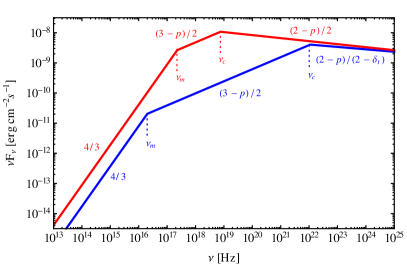
Figure 1: Comparison between two synchrotron spectra: in a homogeneous turbulence of strength $\epsilon_{B}=10^{-2}$ (top red curve), and in a decaying microturbulence such that $\alpha_{t}=-0.5$, $\Delta_{\mu}=10^{2}$. For both, the blast parameters are $\gamma_{\rm b}=245$, $n_{-3}=1$ and the injection distribution index $p=2.2$. The regime is slow cooling, and $t_{\rm dyn}<t_{\mu-}$ (corresponding to case 1 of Fig. 4 for the microturbulent model).

Figure 1 presents a concrete example of a spectral energy distribution, comparing the standard prediction for a homogeneous turbulence with $\epsilon_{B}=10^{-2}$ (blue line) to a time evolving microturbulence with $\alpha_{t}=-0.5$, also starting at $\epsilon_{B}=10^{-2}$ (red line), with $\Delta_{\mu}=10^{2}$. Both models assume $\gamma_{\rm b}=245$ corresponding to an observer time $t_{\rm obs}=100\,$s for a blast at $z=1$ with $E_{53}=1$, $n_{-3}=1$, an injection slope $p=2.2$ and a circumburst medium of constant density. Inverse Compton losses are neglected throughout the blast in this example. Figure 1 reveals the characteristic stretch of frequency range, with $\nu_{\rm m}\simeq 2\times 10^{16}\,$Hz for the dynamical microturbulent model (resp. $\nu_{\rm m}\simeq 2.3\times 10^{17}\,$Hz in the homogeneous turbulence) and $\nu_{\rm c}\simeq 1.1\times 10^{22}\,$Hz (resp. $\nu_{\rm c}\simeq 7.6\times 10^{18}\,$Hz). The frequency $\nu_{\mu+}=2\times 10^{27}\,$Hz lies outside the range of Fig. 1.

For the above case of slow cooling, the spectral indices at low and intermediate frequencies, respectively $\beta=1/3$ and $\beta=-(1-p)/2$ (with $F_{\nu}\propto t^{\alpha}\nu^{-\beta}$) remain unaffected in the presence of decaying microturbulence. However the temporal index $\alpha$ is modified in these cases, even at low frequencies, which opens the possibility of testing such cases through the temporal behavior of an early follow-up in the optical. Section 3.2 below offers a comparison of such spectra with the observed light curve of GRB090510. Regarding the fast cooling part of the electron population, both the spectral and temporal indices are modified, see Table 1 for their detailed values. See also Fig. 4 for an illustration of possible synchrotron spectra.

Synchrotron self-absorption is negligible at all frequencies shown in this figure, see Sec. A.5 for details.

2.4 Rapidly decaying microturbulence (no inverse Compton losses)

There are two main differences between the synchrotron spectra of gradually vs rapidly decaying microturbulence. In the former case, particles may cool in the decaying microturbulence layer, while in the latter, particles either cool in the undecayed region of short extent, if their Lorentz is sufficiently large, or in the background magnetic field beyond the microturbulent layer otherwise, in the absence of inverse Compton losses that is. This implies in particular that there is no well defined cooling Lorentz factor for the microturbulence. Secondly, as the turbulence decays rapidly, most of the synchrotron power is emitted in the region of largest magnetic power, hence the flux $\nu F_{\nu}$ associated to the microturbulent layer peaks at $\nu_{\mu+}$. At times such that $t_{\rm dyn}>t_{\mu-}$, cooling in the background shock compressed field leads to the emergence of a secondary synchrotron component on top of the former, and one may now define a cooling Lorentz factor in the background compressed field. At frequency $\nu_{\rm m}$, the ratio between these two components is of order $t_{\rm dyn}/t_{\mu-}>1$, at the benefit of the latter. At the exit of the microturbulent layer, the maximal Lorentz factor cannot exceed $\gamma_{\mu+}$, so that the secondary component cuts-off at most at $\nu_{\rm p}\left[\gamma_{\mu+};B_{\rm d}\right]$, which falls short of the GeV range, see the discussion in Sec. 3.1. In practice, this suggests that most of the low energy emission in the optical and X-ray domains result from cooling in the background field, while the highest energy emission can be attributed to the presence of the microturbulence.

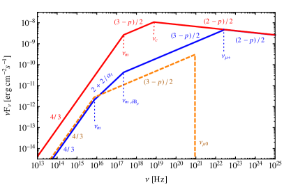
Figure 2: Same as Fig. 1, now comparing the synchrotron spectrum in a homogeneous turbulence of strength $\epsilon_{B}=10^{-2}$ (top red curve), with a decaying microturbulence such that $\alpha_{t}=-1.8$, $\Delta_{\mu}=2.7\times 10^{4}$ (bottom blue curve). For both, the blast parameters are $\gamma_{\rm b}=245$, $n_{-3}=1$ and the injection distribution index $p=2.2$. The orange dashed line represents the secondary synchrotron component associated to cooling in the background shock compressed field (here $B_{\rm u}=10\,\mu$G), which emerges on top of the microturbulent component because $t_{\rm dyn}=1.3t_{\mu-}$ (corresponding to case 2 of Fig. 5). The regime is slow cooling.

Figure 2 presents a concrete example of a spectral energy distribution, comparing the standard prediction for a homogeneous turbulence with $\epsilon_{B}=10^{-2}$ (top red line) to a time evolving microturbulence with $\alpha_{t}=-1.8$, also starting at $\epsilon_{B}=10^{-2}$ (bottom blue curve). The microturbulent layer is such that $\Delta_{\mu}=2.7\times 10^{4}$, corresponding for instance to $\alpha_{\lambda}=3$, $\lambda_{\mu}=30\,c/\omega_{\rm pi}$. The upstream magnetic field $B_{\rm u}=10\,\mu$G and as in Fig. 1, $n_{-3}=1$, $\gamma_{\rm b}=245$, $t_{\rm obs}=100\,$s, $z=1$, which implies in particular that $t_{\rm dyn}=1.3t_{\mu-}$. Therefore, a secondary synchrotron associated to cooling in $B_{\rm d}$ emerges on top of the microturbulent component. The corresponding characteristic frequencies for the microturbulent component are $\nu_{\rm m}\,\simeq\,5.7\times 10^{15}\,$Hz, $\nu_{{\rm m},\delta B_{\mu}}\,\simeq\,2.3\times 10^{17}\,$Hz and $\nu_{\mu+}\,\simeq\,2.8\times 10^{22}\,$Hz; the cut-off frequency of the secondary synchrotron component $\nu_{\mu 0}=0.9\times 10^{21}\,$Hz. In such a scenario, the microturbulent component would dominate in the X-ray and at higher energies, while the secondary component dominates in the optical; at later times, the secondary component would come to dominate as well in the X-ray.

Regarding the spectro-temporal evolution of the flux, one recovers features similar to those discussed above in the case $\alpha_{t}>-1$. In particular, the slow cooling slopes $1/3$ and $(1-p)/2$ remain unaffected, but the temporal index is different when $t_{\rm dyn}<t_{\mu-}$, and for the fast cooling part of the electron population, both spectral and temporal indices are affected by $\alpha_{t}$. The detailed values of $\alpha$ and $\beta$ are given in Table 2 in Appendix A. See also Figs. 5 and 6 for an illustration of the spectral shapes of the synchrotron spectra.

Synchrotron self-absorption is negligible at all frequencies shown in this figure, see Sec. A.5 for details.

2.5 Strong inverse Compton losses

Accounting for inverse Compton losses modifies of course the cooling history of the particle. The importance of inverse Compton losses is generally quantified through the $Y$ Compton parameter, which may be written in a first approximation (e.g. Sari & Esin 2001, Wang et al. 2010) as

$$Y(\gamma)\left[1+Y(\gamma)\right]\,\simeq\,\frac{\epsilon_{e}}{\epsilon_{B}}\frac{\nu F_{\nu}\left[\nu_{\rm KN}(\gamma)\right]}{\nu F_{\nu}\left(\nu_{\rm peak}\right)}f_{\rm cool}\ ,$$ (19)

where the notation $Y(\gamma)$ indicates that $Y$ in general depends on the Lorentz factor of the particle, due to Klein-Nishina effects. These latter are quantified through the ratio of $\nu F_{\nu}\left[\nu_{\rm KN}(\gamma)\right]$, i.e. the synchrotron flux at the frequency at which Klein-Nishina suppression becomes effective, to the peak of the synchrotron flux, $\nu F_{\nu}\left(\nu_{\rm peak}\right)$. Finally, the factor $f_{\rm cool}$ denotes the fraction of cooling electrons, $\simeq 1$ for fast cooling, $\simeq\left(\gamma_{\rm c}/\gamma_{\rm m}\right)^{1-s}$ for slow cooling. The double dependence of $Y$ on Lorentz factor $\gamma$ and distance to the shock front (through $\delta B$) that arises in the present model renders this problem quite complex. To simplify this task, it is assumed here that inverse Compton losses dominate everywhere throughout the blast. This would occur for instance, if $\epsilon_{e}>\epsilon_{B}$ in the undecayed part of the microturbulent layer (a generic assumption), if $f_{\rm cool}$ does not lie too far below unity, and at energies such that Klein-Nishina effects can be neglected. Under such conditions, one may expect $Y>1$ everywhere else, because the magnetic field decays away from the shock.

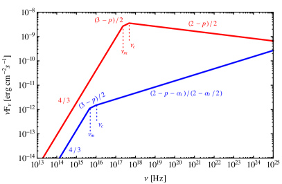
Figure 3: Same as Fig. 1, now comparing the synchrotron spectrum in a homogeneous turbulence of strength $\epsilon_{B}=10^{-2}$ (top red curve) including inverse Compton losses with $Y=3$, with a decaying microturbulence such that $\alpha_{t}=-0.8$, $\Delta_{\mu}=10^{2}$, also including inverse Compton losses with $Y_{\mu}=3$ (bottom blue curve). For both, the blast parameters are $\gamma_{\rm b}=245$, $n_{-3}=1$ and the injection distribution index $p=2.2$. Here $t_{\rm dyn}\,\ll\,t_{\mu-}$ (corresponding to case 1 of Fig. 7). The regime is slow cooling.

In the presence of inverse Compton losses, one can always define a cooling Lorentz factor $\gamma_{\rm c}$ irrespectively of the value of $\alpha_{t}$. As the cooling history of the particles is modified, so are the spectral slopes in the fast cooling part if $\alpha_{t}>-4/(p+1)$, and also at low frequencies if $\alpha_{t}<-4/(p+1)$. In this latter situation indeed, the synchrotron spectrum is dominated at high frequencies by a slow cooling spectrum in the undecayed microturbulence, with a low energy extension from $\nu_{\rm m}$ to $\nu_{{\rm m},\delta B_{\mu}}$ [see Eq. 69] with slope $1+2/\alpha_{t}$. At low frequencies, a secondary component associated to cooling in the background compressed field emerges if both $t_{\rm dyn}<t_{\mu-}$ and $\gamma_{\rm m}<\gamma_{\mu-}$. The synchrotron spectra for $\alpha_{t}>-1$ share features similar to those discussed in Sec. 2.3, up to the modifications of the spectro-temporal indices. One noteworthy distinction is the fact that the fast cooling spectral index has become $-(p+\alpha_{t}/2)/(2-\alpha_{t}/2)$, which may become larger than $-1$ if $\alpha_{t}<2-p$, in which case most of the power lies at $\nu_{\mu+}$. This may be attributed to a scaling of the Compton parameter with frequency: higher frequencies correspond to higher Lorentz factors, hence to cooling in a region of higher magnetic field, where the Compton parameter is smaller, which implies that a smaller fraction of the particles energy is channeled into the inverse Compton component.

Figure 3 presents a concrete example of a spectral energy distribution, comparing the standard prediction for a homogeneous turbulence with $\epsilon_{B}=10^{-2}$ including inverse Compton losses with $Y=3$ (top red line) to a time evolving microturbulence with $\alpha_{t}=-0.8$, also starting at $\epsilon_{B}=10^{-2}$, with $\Delta_{\mu}=10^{2}$ and $Y_{\mu}=3$ (bottom blue curve). For this case, $t_{\rm dyn}\,\ll\,t_{\mu-}$, corresponding to case 1 of Fig. 7; other parameters remain unchanged compared to previous figures. The corresponding characteristic frequencies for the microturbulent component are $\nu_{\rm m}\,\simeq\,4.7\times 10^{15}\,$Hz, $\nu_{\rm c}\,\simeq\,1.0\times 10^{16}\,$Hz and $\nu_{\mu+}\,\simeq\,1.3\times 10^{26}\,$Hz.

The spectro-temporal indices $\alpha$ and $\beta$ are given in Table 3 for $\alpha_{t}>-4/(p+1)$ and 4 in the opposite limit $\alpha_{t}<-4/(p+1)$. The generic spectral shapes are illustrated in Figs. 7 and 8 for these two cases, respectively.

Here as well, synchrotron self-absorption is negligible at all frequencies shown in this figure, see Sec. A.5 for details.

3 Discussion

Most of the discussion so far has ignored the characteristic frequency associated to the maximal energy of the acceleration process. Yet, the production of GeV photons through synchrotron radiation of electrons already push ultra-relativistic Fermi acceleration to its limits, as discussed e.g. in Piran & Nakar (2010), Kirk & Reville (2010), Barniol-Duran & Kumar (2010, 2011a), Lemoine & Pelletier (2011c), Sagi & Nakar (2012), Bykov et al. (2012). These studies assume a homogeneous downstream turbulence, with either microscale high power turbulence or simply a shock compressed magnetic field. Section 3.1 extends these calculations to an evolving microturbulence, which brings in further constraints and new phenomena. A brief comparison with the light curve of GRB090510, which so far provides the earliest follow-up in the optical through GeV, is then proposed.

3.1 Acceleration to high energies

The maximal energy is determined through the comparison of the acceleration timescale $t_{\rm acc}$ to other relevant timescales, e.g. the energy loss and dynamical timescales. Given that the energy gain per Fermi cycle is of order 2 (Gallant & Achterberg 1999, Achterberg et al. 2001, Lemoine & Pelletier 2003), it suffices to compare in each respective rest frame the downstream $t_{\rm res|d}$ and the upstream $t_{\rm res|u}$ residence times to the other timescales.

3.1.1 Upstream

The upstream residence time $t_{\rm res|u}\simeq 5t_{\rm L,0|u}/\gamma_{\rm sh}$ (Lemoine & Pelletier 2003) – assuming that the particle only interacts with the background field – where $t_{\rm L,0}=\gamma_{\rm b}\gamma_{e}m_{e}c/(eB_{\rm u})$ and $\gamma_{e}$ represents the particle Lorentz factor in the downstream frame, $\gamma_{\rm sh}=\sqrt{2}\gamma_{\rm b}$. Considering this residence time leads to a conservative limit on the maximal energy, because scattering in the microturbulent field seeded in the shock precursor should also play a role, see Plotnikov et al. (2012) for further discussion on this issue. Comparing the above residence time to the age of the shock wave $r/c$ then leads to a maximal Lorentz factor (downstream frame)

$$\gamma_{\rm max}^{(a)}\,\simeq\,1.2\times 10^{9}B_{-5}E_{53}^{1/4}n_{-3}^{-1/4}t_{2}^{1/4}z_{+,0.3}^{-1/4}\ .$$ (20)

Depending on the dynamics of the microturbulence downstream, this maximal Lorentz leads to to photons of energy

$$\epsilon_{\gamma,{\rm max}}^{(a)}\,\simeq\,1\,{\rm TeV}B_{-5}^{2}E_{53}^{3/4}n_{-3}^{-1/4}t_{2}^{-1/4}z_{+,0.3}^{-3/4}\epsilon_{B,-2}^{1/2}\ ,$$ (21)

through radiation in the $\delta B_{\mu}$ field, or

$$\epsilon_{\gamma,{\rm max}}^{(a)}\,\simeq\,30\,{\rm GeV}B_{-5}^{3}E_{53}^{3/4}n_{-3}^{-1/4}t_{2}^{-1/4}z_{+,0.3}^{-3/4}\ ,$$ (22)

if the particle radiates in the background shock compressed field $B_{\rm d}$, as proposed in Barniol-Duran & Kumar (2010, 2011a). This latter case applies in particular if $\alpha_{t}<-1$, $\gamma_{\rm max}^{(a)}<\gamma_{\mu+}$ and if downstream inverse Compton losses can be neglected. If however, $\gamma_{\rm max}^{(a)}>\gamma_{\mu+}$, then the particle radiates in the stronger $\delta B_{\mu}$, while if $\alpha_{t}>-1$ and $\gamma_{\rm max}^{(a)}<\gamma_{\mu+}$, the particle radiates in a field of strength $\delta B\simeq\delta B_{\mu}\left(\gamma_{\rm max}^{(a)}/\gamma_{\mu+}\right)^{-\delta_{t}}$, which for these high energies lies in practice close to $\delta B_{\mu}$. For instance, if $\alpha_{t}=-0.5$, one finds

$$\epsilon_{\gamma,{\rm max}}^{(a)}\,\simeq\,0.55\,{\rm TeV}B_{-5}^{2.5}E_{53}n_{-3}^{-1/4}t_{2}^{-0.5}z_{+,0.3}^{-0.5}\Delta_{\mu,2}^{0.5}\epsilon_{B,-2}\ .$$ (23)

Equation 22 matches the “confinement” estimates of Piran & Nakar (2010), Barniol-Duran & Kumar (2011a), who considered only a shock compressed background field in the downstream, while the other estimates Eqs. 21, 23 hold in the present more realistic setting because of the high value of magnetic field behind the shock front.

Note that the particle is actually confined close to the shock front, because in the ultra-relativistic regime, the shock front never lags further than $ct_{\rm res|u}/\gamma_{\rm sh}^{2}$ behind the particle; escape can only take place through the boundaries, but this would lead to a less stringent condition on maximal energy than the above age constraint, see e.g. Bykov et al. (2012).

The above suggests that the upstream magnetic field can lie well below $10\,\mu$G and yet lead to the production of multi-GeV photons because the maximal Lorentz factor particles cool in a strong field, close to the microturbulent value $\delta B_{\mu}$ behind the shock. Furthermore, if one neglects altogether the upstream magnetic field, the discussion in Plotnikov et al. (2012) suggests that scattering the microturbulent field generated in the shock precursor may lead to Lorentz factors sufficiently large to produce GeV photons through synchrotron radiation in $\delta B_{\mu}$.

Li & Waxman (2006) and Li & Zhao (2011) have argued that the comparison of the upstream residence time with the timescale for inverse Compton losses imposes a stringent lower bound on the upstream magnetic field, suggesting an efficient amplification of the latter. More specifically, Li & Zhao (2011) find that $1\,{\rm mG}\,n_{0}^{9/8}\,\lesssim\,\bar{B}_{\rm u}\,\lesssim\,100\,{\rm mG}\,n_{0}^{3/8}$ (with $\bar{B}_{\rm u}$ denoting the total magnetic field upstream of the blast) is imposed by the synchrotron model of $Fermi-$LAT bursts with extended GeV emission. These bounds have been challenged in Barniol-Duran & Kumar (2011b) and Sagi & Nakar (2012). Nevertheless, such bounds agree well with the general picture that microinstabilities self-generate a microturbulent field in the shock precursor, which is then transmitted downstream and there forms the microturbulent layer. One expects that in the shock precursor, the microturbulent field $\bar{B}_{\rm u}\sim\delta B_{\mu}/\gamma_{\rm b}$ (as measured in the upstream frame), in which case one finds $\bar{B}_{\rm u}\sim 1\,{\rm mG}\,\epsilon_{B,-2}^{1/2}n_{-3}^{1/2}$. This field satisfies the constraints of Li & Zhao (2011).

3.1.2 Downstream

Consider now the situation downstream, which leads to much more severe contraints on $\epsilon_{\gamma,\rm max}$ through the comparison of $t_{\rm res|d}$ with the timescale of energy loss. Out of commodity and simplicity, the limit on the maximal energy is often quoted with a Bohm estimate $t_{\rm res|d}\simeq\kappa_{\rm B}t_{\rm L}$, with $t_{\rm L}=(\gamma_{e}m_{e}c)/(e\delta B)$ in the downstream frame. Ignoring inverse Compton losses, this leads to

$$\gamma_{\rm max}^{(b)}\,\simeq\,2.1\times 10^{8}\kappa_{\rm B}^{-1/2}t_{2}^{3/16}E_{53}^{-1/16}n_{-3}^{-3/16}\epsilon_{B,-2}^{-1/4}\ ,$$ (24)

assuming for the moment that $\delta B$ is homogeneous, with strength characterized by $\epsilon_{B}$. This leads to

$$\epsilon_{\gamma,\rm max}^{(b)}\,\simeq\,30\,{\rm GeV}\,\kappa_{\rm B}^{-1}E_{53}^{1/8}t_{2}^{-3/8}n_{-3}^{-1/8}\ ,$$ (25)

which matches the estimate of Piran & Nakar (2010) up to a factor 2. However, this estimate must be corrected for two effects: (1) the Bohm approximation likely breaks down at these large Lorentz factors; (2) the evolution of the microturbulence away from the shock front modifies the scattering rate of the particles.

The Bohm approximation for $t_{\rm res|d}$ fails at the maximal Lorentz factors because

$$\frac{r_{\rm L}\left(\gamma_{\rm max}^{(b)}\right)}{\lambda_{\mu}}\,\simeq\,1.7\times 10^{2}\,\lambda_{\mu,1}t_{2}^{9/16}E_{53}^{-3/16}n_{-3}^{-1/16}\epsilon_{B,-2}^{-3/4}\gg 1\ ,$$ (26)

for a Lorentz factor given by Eq. 24. This implies that the particle only suffers a random small angle deflection of order $\lambda_{\mu}/r_{\rm L}$ as it crosses a coherence cell of size $\lambda_{\mu}=10\lambda_{\mu,1}c/\omega_{\rm pi}$, hence the residence timescale is rather given as: $t_{\rm res|d}\simeq\kappa_{\rm sc}\left(r_{\rm L}/\lambda_{\mu}\right)r_{\rm L}$, much larger than the above Bohm estimate. This of course reduces significantly the maximal energy of photons (Kirk & Reville 2010, Lemoine & Pelletier 2011c, Plotnikov et al. 2012). At the present time, one cannot exclude that the spectrum of turbulent modes extends to wavenumbers $k\sim r_{\rm L}^{-1}$ that would allow gyroresonant interactions in the downstream; whether or not this happens depends on the physics of instabilities in the far upstream, which are still debated. Were this the case, the Bohm estimate should nevertheless be corrected by a factor that accounts for the diminished magnetic power at those resonant scales, compared to the maximum power at $\lambda_{\mu}^{-1}$. In order to obtain a conservative estimate of the maximal energy, one should therefore rely on the above $t_{\rm res|d}\propto r_{\rm L}^{2}$. Comparing this residence timescale with the synchrotron loss time, this would lead to a maximal Lorentz factor

$$\gamma_{\rm max}^{(c)}\,\simeq\,3.9\times 10^{7}\,\kappa_{\rm sc}^{-1/3}\lambda_{\mu,1}n_{-3}^{-1/6}\ ,$$ (27)

corresponding to a maximum photon energy

$$\epsilon_{\gamma,\rm max}^{(c)}\,\simeq\,0.9\,{\rm GeV}\,\kappa_{\rm sc}^{-2/3}E_{53}^{1/4}n_{-3}^{-1/12}\lambda_{\mu,1}^{2/3}\epsilon_{B,-2}^{1/2}t_{2}^{-3/4}\ ,$$ (28)

provided the radiation takes place in the microturbulent field of strength $\delta B_{\mu}$. If radiation were to take place in the background shock compressed field $B_{\rm d}$, the maximal photon energy would rather be

$$\epsilon_{\gamma,\rm max}^{(c)}\,\simeq\,30\,{\rm MeV}\,\kappa_{\rm sc}^{-2/3}E_{53}^{1/4}n_{-3}^{-7/12}\lambda_{\mu,1}^{2/3}B_{-5}t_{2}^{-3/4}\ .$$ (29)

However, once the evolution of the microturbulence is accounted for, these estimates are modified towards more optimistic values. Consider first the scaling of $r_{\rm L}/\lambda$, with $r_{\rm L}$ now designing the gyroradius in the local magnetic field, and $\lambda$ the coherence length of this local magnetic field. Then

$$\frac{r_{\rm L}}{\lambda}\,\propto\,t^{-\alpha_{t}/2-1/\alpha_{\lambda}}\ .$$ (30)

With $\alpha_{\lambda}\sim 2-3$, the following qualitative picture emerges. If the turbulence decays gradually, meaning $\alpha_{t}\gtrsim-1$, the coherence length increases more rapidly away from the shock front than the magnetic field loses power, so that the scattering timescale tends towards a Bohm scaling (albeit, in a weaker magnetic field) as time increases (see also Katz et al. 2007 for a similar picture). One then obtains (see further below) maximal energy estimates close to the Bohm scaling. If, however, the turbulence decays fast, meaning $\alpha_{t}\lesssim-1$, then the scattering timescale increases with time, possibly faster than $t$ if $\alpha_{t}\lesssim-1-1/\alpha_{\lambda}$, in which case scattering becomes impossible in the decaying part of the microturbulent layer. Furthermore, mirror like interactions in the background shock compressed magnetic field, which lies transverse to the shock normal, do not allow repeated returns to the shock front (Lemoine et al. 2006, see also Sec. 3.3). The particles must then scatter in the undecayed microturbulent field, if $\alpha_{t}\lesssim-1$, in which case the maximal energy is then determined by the comparison of $t_{\rm res|d}$ to $t_{\mu+}$. These two scenarios are examined in turn.

Assume first $\alpha_{t}\gtrsim-1$, meaning more specifically $\alpha_{t}>-2/\alpha_{\lambda}$. Then the small angle scattering timescale $t_{\rm res|d}\propto t^{-\alpha_{t}-1/\alpha_{\lambda}}$, which must be compared to the synchrotron loss time $t_{\rm syn}\propto\gamma_{\rm max}^{-1}\delta B_{\mu}\left(t_{\rm res|d}/t_{\mu+}\right)^{-\alpha_{t}}$, where the last factor accounts for the evolution of the magnetic field strength with time, outside the undecayed layer. This leads to

$$\gamma_{\rm max}^{(d)}\simeq\gamma_{\mu+}\left[\frac{r_{\rm L}(\gamma_{\mu+})^{2}}{\lambda_{\mu}\,ct_{\mu+}}\right]^{-(1+\alpha_{t})/(3+3\alpha_{t}+1/\alpha_{\lambda})}\ .$$ (31)

The term within the brackets can be rewritten in a more compact way as $4\gamma_{\mu+}^{3}r_{e}\lambda_{\mu}^{-1}/9$, with $r_{e}$ the classical electron radius, so that in the limit $\alpha_{\lambda}\rightarrow+\infty$, one recovers the estimate $\gamma_{\rm max}^{(c)}$ in a homogeneous microturbulence. The fiducial values $\alpha_{t}=-0.5$ and $\alpha_{\lambda}=2$ discussed previously lead however to

$$\gamma_{\rm max}^{(d)}\,\sim\,1.2\times 10^{8}\,\Delta_{\mu,2}^{-0.25}E_{53}^{-0.06}n_{-3}^{-0.19}\epsilon_{B,-2}^{-0.25}\lambda_{\mu,1}^{0.25}t_{2}^{0.19}\ ,$$ (32)

which, through synchrotron radiation in a magnetic field of strength $\delta B\simeq\delta B_{\mu}\left(\gamma_{\rm max}^{(d)}/\gamma_{\mu+}\right)^{-\delta_{t}}$ leads to photons of typical energy

$$\epsilon_{\gamma,\rm max}^{(d)}\,\simeq\,2\,{\rm GeV}\,E_{53}^{0.22}\lambda_{\mu,1}^{0.63}\Delta_{\mu,2}^{-0.13}n_{-3}^{-0.094}\epsilon_{B,-2}^{0.38}t_{2}^{-0.66}\ .$$ (33)

One should stress that this result depends on the particular value of $\alpha_{t}$ and $\alpha_{\lambda}$, but for the above fiducial values, it remains close to the Bohm estimate and allows the production of GeV photons for conservative assumptions. Note finally that the stretching of the coherence length with time does not imply that the particles of Lorentz factor $\gamma_{\rm max}^{(d)}$ suffer gyroresonant interactions away from the shock, nor does it require that the turbulent power spectrum extends over many decades. For the above fiducial values, the particles interact with modes of wavelength $l\,\sim\,30\lambda_{\mu}\,\ll r_{\rm L}$.

In a fast decaying scenario, meaning more exactly $\alpha_{t}<-1-1/\alpha_{\lambda}$, scattering must take place in the undecayed part of the microturbulent layer, otherwise the particles would not see the microturbulent layer and Fermi acceleration would not take place. The comparison $t_{\rm res|d}<t_{\mu+}$ leads to

$$\gamma_{\rm max}^{(e)}\,\simeq\,4\times 10^{6}\,\kappa_{\rm sc}^{-1/2}E_{53}^{1/8}\lambda_{\mu,1}^{1/2}\epsilon_{B,-2}^{1/2}n_{-3}^{-1/8}t_{2}^{-3/8}z_{+,0.3}^{3/8}\Delta_{\mu,2}^{1/2}\ ,$$ (34)

which would lead to ${\cal O}(10)\,$MeV photons only, even through radiation in a field as strong as $\delta B_{\mu}$. To reach the GeV range, ceteris paribus, one needs to increase the spatial extent of the undecayed microturbulence, i.e. to increase $\Delta_{\mu,2}$ by $2-3$ orders of magnitude. For $\Delta_{\mu}\gtrsim 10^{4}$, indeed, $\gamma_{\rm max}^{(e)}\gtrsim\gamma_{\mu+}$, so that the particle both scatters and cools in the undecayed part of the microturbulent layer.

To summarize, the above analysis of scattering and maximal photon energies leads to the following qualitative picture. If the turbulence decays gradually, the particles scatter while the microturbulence decays and the maximal energy of the photons typically falls in the GeV range for fiducial parameters and rather conservative estimates of the scattering properties. If, however, the turbulence decays rapidly, GeV photons can only be produced if the undecayed part of the turbulent layer extends far enough to accomodate both the scattering and the cooling of the maximal energy electrons in that layer. This latter requirement places strong constraint on the parameter $\Delta_{\mu}$ that characterizes for how long the undecayed turbulence can survive. Requisite values can be obtained if, for instance, $\lambda_{\mu}\sim 30c/\omega_{\rm pi}$ and $\alpha_{\lambda}\sim 3$, which cannot be excluded at present. Finally, it has also been noted that the constraints on the upstream residence time are much weaker if the maximal energy electrons can radiate in a field close to $\delta B_{\mu}$. In practice, this implies that the value of the upstream magnetic field is not well constrained. This alleviates the apparent strong magnetization problem discussed in He et al. (2011).

3.2 Early GRB light curves

Section 2 together with Appendix A have emphasized the differences between the standard synchrotron spectra for homogeneous turbulence and those calculated with the account of decay of the microturbulence. This Section confronts such signatures with the observational data on GRB090510, which so far has provided the earliest follow-up on a broad spectral range, with near simultaneous detection in the optical, X range and GeV range (de Pasquale et al. 2010; Ukwatta et al. 2009; Guiriec et al. 2009; Ackermann et al. 2010; Longo et al. 2009; Hoversten et al. 2009; Golenetskii et al. 2009; Ohmori et al. 2009). This choice is further motivated by the analyses of Barniol-Duran & Kumar (2009, 2010, 2011a) and He et al. (2011), who have argued that the extended emission, from the optical to the GeV range is compatible with an afterglow spectrum calculated without magnetic field generation beyond direct shock compression of the interstellar field. One may also interpret the data with a high magnetization of the blast, closer to the traditional estimates of $\epsilon_{B}$, although it then requires an extraordinarily low upstream density $\lesssim 10^{-6}\,$cm^-3 (e.g. de Pasquale et al. 2009, Corsi et al. 2010); this possibility is not considered here. The model of Barniol-Duran & Kumar (2009, 2010, 2011a) then suggests that magnetic field generation processes are ineffective, and that this burst provides the closest relative to a “clean” relativistic blast wave in a weakly magnetized medium

As discussed in the previous Sections, one should expect that the GeV photons have been produced in the microturbulent layer rather than in the background magnetic field. However, lower energy photons in the optical and in the X range are typically produced by particles of Lorentz $\gamma_{\rm m}$, which lose energy on a much longer timescale than the particles of Lorentz factor $\gamma_{\rm max}$, hence in a weaker magnetic field, possibly the background shock compressed value $B_{\rm d}$. In any case the microturbulence is to play a key role in shaping the spectra from the GeV down to lower energies. This motivates further the search for a signature of this microturbulence.

Unfortunately, the comparison is not straightforward, because of the diversity and complexity of the synchrotron spectra. The quantities that characterize the microturbulence appear as new free parameters from the point of view of phenomenology, hence they enlarge the dimensionality of parameter space and add degeneracy. For this reason, the following does not attempt to fit accurately the light curves in the GeV, X-ray and optical, but rather accomodates the different spectro-temporal indices in the different time domains of the observations. The key observation of the Barniol-Duran & Kumar (2009, 2010, 2011a) interpretation is that the spectrum is produced in a slow cooling regime, and that in the case of GRB090510, $\nu_{\rm m}$ transits across the optical at $10^{3}\,$s, in order to produce the observed break. Once this condition is satisfied, and provided spectro-temporal indices match the observed values, one obtains a satisfactory fit to the light curves (as it has been checked). The following discussion reveals that the current data do not allow one to pick out a preferred model, meaning conversely that it is possible to reproduce the salient features of the Barniol-Duran & Kumar (2009, 2010, 2011a) model with concrete characterizations of the microturbulence. Each model leads to rather specific signatures that might be identified with further higher accuracy and earlier observations. Some of these signatures are pointed out in the following, although more work is needed to define an observation strategy capable of pinpointing the characteristics of the microturbulence.

GRB090510 is a short burst at redshift $z=0.92$ whose light curve is characterized as follows: emission is seen in the LAT range up to $\simeq 100\,$s, with spectro-temporal indices $\alpha_{\rm GeV}\simeq 1.4$, $\beta_{\rm GeV}\simeq 1.1$; X-ray and optical follow-up start at about this time; from $\simeq 100\,$s to about $1.5\times 10^{3}\,$s, $\alpha_{\rm X}\simeq 0.74$, increasing to $2.2$ afterwards, while $\beta_{\rm X}\simeq 0.5-0.8$; $\alpha_{\rm opt}\simeq-0.5$ before $10^{3}\,$s, then $1.1$ afterwards. The late time evolution beyond $10^{3}\,$s is more difficult to reproduce, in particular the steepening of the X-ray lightcurve, which is attributed by He et al. (2011) to sideways expansion, but which does not match the apparent shallower decay in the optical up to $2\times 10^{4}\,$s (Nicuesa Guelbenzu et al. 2012).

To compare this light curve with the afterglow computed in App. A, consider first the possiblity of $\alpha_{t}>-1$ (gradual decay) without inverse Compton losses. The latter assumption has been discussed at length in He et al. (2011). As shown in Fig. 4, the spectral shape of the synchrotron spectrum in the slow cooling limit with $\alpha_{t}>-1$ retains the same form as the standard afterglow, but the values of the characteristic frequencies and therefore the time dependences are modified. Therefore, $\beta_{\rm X}\simeq 0.6$ if $\nu_{\rm m}<1\,{\rm keV}\,<\,\nu_{\rm c}$ as observed. In the model of Barniol-Duran & Kumar (2010), He et al. (2011), $\nu_{\rm c}$ lies below the LAT range, so that

$$\beta_{\rm GeV}\simeq-\frac{p-\alpha_{t}(1-2p)/2}{2+3\alpha_{t}/2}\ ,$$ (35)

which takes values between $-1.10$ and $-1.00$ for $p=2.2$ and $\alpha_{t}\in[0,-1]$, in good agreement with the data, although the influence of $\alpha_{t}$ is too weak to provide significant constraints. The temporal slope in the GeV range also depends mildly on $\alpha_{t}$, taking values from $\alpha=1.15$ at $\alpha_{t}=0$ ($p=2.2$) to $\alpha=1.25$ at $\alpha_{t}=-1$ ($p=2.2$). It fits with the observations, given that the measured slope may be contaminated by prompt GeV emission, see the discussion in He et al. (2011). The best probes for $\alpha_{t}$ remain the temporal slopes in the X and optical domains: $\alpha$ takes values between $0.9$ and $1.4$ in the X range (for $p=2.2$), and between $-0.50$ and $-0.30$ ($p=2.2$) in the optical when $1\,{\rm eV\,}<\nu_{\rm m}$. Current data do not allow a precise determination of $\alpha_{t}$, but it may be noted that the fiducial value $\alpha_{t}=-0.5$ fits well the data. Finally, requiring $\nu_{\rm m}\sim 1\,$eV at $10^{3}\,$s determines $\alpha_{t}$ as a function of the other parameters. For the fiducial values characterizing the turbulence, $n\sim 10^{-3}\,$cm^-3 and $B_{\rm d}\lesssim 1\,\mu$G, $\nu_{\rm m}=\nu_{\rm p}\left[\gamma_{\rm m};\delta B(t_{\rm dyn})\right]$ because the turbulence has not had time yet to relax to the background magnetic field $B_{\rm d}$. Then

$$\nu_{\rm m} \,\simeq\, 2.3\times 10^{17}\,{\rm Hz}\,e^{4.851\alpha_{t}/(1+\alpha_{t})}E_{53}^{1/2+\alpha_{t}/16}n_{-3}^{3\alpha_{t}/16}$$ (36)

$$\,\,\,\times\Delta_{\mu,2}^{-\alpha_{t}/2}\epsilon_{B,-2}^{1/2}\epsilon_{e,-0.3}^{2}t_{2}^{-3/2+5\alpha_{t}/16}\ ,$$

so that $\nu_{\rm m}\sim 1\,$eV at $10^{3}\,$s implies $\alpha_{t}=-0.6$ up to small logarithmic corrections. It is somewhat remarkable that the value of $\alpha_{t}$ falls close to the fiducial value discussed previously. Also, one may note that the upstream magnetic field does not enter Eq. 36, because the particles actually cool in the decaying microturbulence. One may verify that the above choice of parameters gives a light curve in good agreement with the observed data, except for the late time shallow decay in the optical mentioned above.

To pursue this comparison, consider now the possibility that $-4/(p+1)<\alpha_{t}<-1$. The fast decay of the microturbulence in this case actually mimics somewhat the scenario originally proposed by Barniol-Duran & Kumar (2010, 2011a): the particles get accelerated in a microturbulent layer behind the shock front but cool where the microturbulence has died away. Although, as discussed in some details in Sec. 3.1, it appears necessary to require that the particles of Lorentz factor $\gamma_{\rm max}$ actually cool in the microturbulent layer in order to produce the GeV photons, in other words $\gamma_{\mu+}\lesssim 4\times 10^{7}$ at $t_{\rm obs}\sim 100\,$s, which implies

$$\Delta_{\mu}\gtrsim 10^{4}E_{53}^{-1/4}n_{-3}^{-1/4}\epsilon_{B,-2}^{-1}t_{2}^{1/4}\ ,$$ (37)

or to put it more simply, that the undecayed part of the microturbulent layer with $\epsilon_{B,-2}\sim 10^{-2}$ extends for some $10^{4}$ skin depths at least.

Two different behaviors can be observed, depending on the ratio $t_{\rm dyn}/t_{\mu-}$, i.e. whether the turbulence has relaxed down to $B_{\rm d}$, in which case a synchrotron component associated to $B_{\rm d}$ would emerge on top of the microturbulent synchrotron spectrum. The maximum value of $t_{\rm dyn}/t_{\mu-}$ is obtained for $\alpha_{t}\rightarrow-4/(p+1)\simeq-1.3$:

$$\frac{t_{\rm dyn}}{t_{\mu-}}\,\sim\,0.3B_{-5}^{1.53}E_{53}^{1/8}n_{-3}^{-0.39}\epsilon_{B,-2}^{-0.77}\Delta_{\mu,4}^{-1}t_{2}^{5/8}\ ,$$ (38)

so that both possibilities have to be envisaged. If $t_{\rm dyn}<t_{\mu-}$ up to late times, and $\nu_{\rm m}<1\,{\rm eV}\,<\,\nu_{\mu 0}$ beyond $10^{3}\,$s, the optical flux should decay fast with $\alpha_{\rm opt}\simeq 1.4\rightarrow 1.6$, which disfavors this possibility. If now $t_{\rm dyn}>t_{\mu-}$ at some point, the synchrotron component produced by the cooling of particles in $B_{\rm d}$ emerges and dominates over that produced by the microturbulence, at least at low frequencies (optical, X). This $B_{\rm d}$ component cuts off at $\nu_{\mu 0}\,\equiv\,\nu_{\rm p}\left[\gamma_{\mu+};B_{\rm d}\right]$, as discussed in Sec. 2.4; $\nu_{\mu 0}$ increases with time, and for reasonable choices of parameters, it lies above the X range. At the time at which $t_{\rm dyn}=t_{\mu-}$, however, the temporal decay slope in the X range changes from $(6p-1)/8$ (due to cooling in the microturbulence) to $3(p-1)/4$, which implies a change from steep to shallow, which is not observed. Therefore, this scenario is disfavored as well. It is difficult at the present to rule it out clearly, as other effects, due to jet breaking for instance, could complicate the temporal scaling.

Consider now the possibility $-3<\alpha_{t}<-4/(p+1)$, without inverse Compton losses as above. Similar considerations regarding the maximal energy suggests that $\gamma_{\mu+}\lesssim 4\times 10^{7}$, implying $\Delta_{\mu}\gtrsim 10^{4}$. The turbulence decays fast so that, for a reasonable choice of parameters, e.g. $\alpha_{t}\lesssim-1.5$, $n_{-3}\sim 1$, $B_{-5}\sim 1$, the condition $t_{\rm dyn}>t_{\mu-}$ may be fulfilled at $t_{\rm obs}\gtrsim 100\,$s. This implies that the background synchrotron component emerges on top of the microturbulent synchrotron spectrum, and dominates at low frequencies. One then recovers the standard afterglow spectrum proposed by Barniol-Duran & Kumar (2010), except that the GeV photons are produced in the microturbulent layer. In the GeV range, the indices $(\alpha,\beta)$ match the standard predictions for the fast cooling population and thus agree with the data; the overall afterglow provides a satisfactory fit to the available data. In order to discriminate this model, one would need to access the early light curve in the frequency range $\nu_{\rm m}<\nu<\nu_{\rm m,\delta B_{\mu}}$ (i.e. X-ray) in which both the spectral and temporal indices evolves strongly with $\alpha_{t}$: $(\alpha,\beta)$ go from $(1.6,0.5)$ to $(0.1,-0.4)$ as $\alpha_{t}$ goes from $-1.3$ to $-3$. For reference, $\nu_{\rm m,\delta B_{\mu}}\simeq 2.3\times 10^{17}\,{\rm Hz}\,E_{53}^{1/2}\epsilon_{B,-2}^{1/2}\epsilon_{e,-0.3}^{2}t_{2}^{-3/2}$.

Another interesting solution arises in this scenario when $t_{\rm dyn}<t_{\mu-}$ up to late times. This may be realized if $B_{-5}\ll 1$ for instance. Then the frequency $\nu_{\rm m}=\nu_{\rm p}\left[\gamma_{\rm m};\delta B(t_{\rm dyn})\right]$ transits through the optical at $10^{3}\,$s if $\alpha_{t}\sim-1.5$, as required. During the interval $10^{3}-10^{4}\,$s, the optical lies in the range $\nu_{\rm m}-\nu_{{\rm m},\delta B_{\mu}}$ with $(\alpha,\beta)=-\left[(24+7\alpha_{t})/(8\alpha_{t}),1+2/\alpha_{t}\right]$. To reconcile $\alpha$ with $\alpha_{\rm opt}\sim 0.8$ (Nicuesa Gulbenzu et al. 2012), one would need to impose $\alpha_{t}\sim-1.8$, while $\beta_{\rm opt}\sim 0.9$ at that time rather requires $\alpha_{t}\simeq-1.1$. Thus $\alpha_{t}\simeq-1.5$ provides a compromise, which is marginally acceptable by the data, that presents the clear advantage of a shallower decay in the optical than in the X-ray at a time at which it is observed. At $10^{4}\,$s, $\nu_{{\rm m},\delta B_{\mu}}$ transits across the optical (see its expression above), so that the optical and the X-ray domains decline alongside at later times.

Whichever ratio $t_{\rm dyn}/t_{\mu-}$ is considered, the model with $\alpha_{t}<-4/(p+1)$ predicts a clear signature in the early optical lightcurve, with $\alpha_{\rm opt}=-1/8$ when $1\,{\rm eV}\,<\,\nu_{\rm m}$, which leads to a mild growth the optical flux. De Pasquale et al. (2010) report $\alpha_{\rm opt}=-0.5^{+0.11}_{-0.13}$ between $10^{2}\,$s and $10^{3}\,$s, while Nicuesa Gulbenzu et al. (2012) rather indicate $\alpha_{\rm opt}=-0.2\pm 0.2$, therefore it is not possible to rule out or confirm this model at present.

Consider finally the possiblity of strong inverse Compton losses. As before, it is assumed here that these losses dominate throughout the blast, although a more realistic model should include the possibility of weak inverse Compton losses at the highest energies due to the Klein-Nishina suppression of the cross section. Nevertheless, one may constrain this scenario with the optical and X data, as follows.

The dominance of inverse Compton losses for particles of Lorentz factor $\gamma_{\rm m}$ implies that $\gamma_{\rm c}\sim\gamma_{\rm m}$, since

$$\frac{\gamma_{\rm c}}{\gamma_{\rm m}}\,\simeq\,1.5E_{53}^{-1/2}n_{-3}^{-1/2}\epsilon_{B,-2}^{-1}\epsilon_{e,-0.3}^{-1}\frac{4}{1+Y_{\mu}}t_{2}^{0.5}\ ,$$ (39)

see Eq. 74 for the definition of $Y_{\mu}$. Consider first the possibility $\alpha_{t}>-4/(p+1)$, this implies that $\nu_{\rm m}\lesssim 1\,$keV and $\nu_{\rm c}\lesssim 1\,$keV at $t_{\rm obs}\gtrsim 100\,$s, so the X range always fall in the fast cooling portion. The spectral slope cannot be $-p/2$ in that range, otherwise it could not match the observed $\beta_{\rm X}$; the slope must thus be $-(p+\alpha_{t}/2)/(2-\alpha_{t}/2)$, which fits $\beta_{X}\simeq 0.5-0.8$ only for $\alpha_{t}\sim-0.8\rightarrow-1.3$. In turn, this would imply a positive value of $\alpha_{\rm opt}$ if $\nu_{\rm m}>\nu_{\rm c}$ (fast cooling), so the regime at time $t_{\rm obs}\gtrsim 100\,$s must be that of slow cooling (case 1 or 2 depicted in Fig. 7). One should further require that $\nu_{\rm m}$ goes into the optical at $10^{3}\,$s as before. These features can be achieved for the typical fiducial values considered before, $n_{-3}\sim 1$, $E_{53}\sim 1$, with $\alpha_{t}\sim-0.8\rightarrow-1.3$.

An interesting feature of this scenario is that the ratio $t_{\rm dyn}/t_{\mu-}$ can take values smaller or larger than unity for standard parameters of the microturbulence and $\alpha_{t}\sim-1$. As it depends sensitively on the value of the upstream magnetic field, as $B_{\rm u}^{-2/\alpha_{t}}$, the transition from $t_{\rm dyn}<t_{\mu-}$ (case 1 in Fig. 7) to $t_{\rm dyn}>t_{\mu-}$ (case 2 in Fig. 7) may well occur around $10^{2}-10^{3}\,$s. Once $t_{\rm dyn}/t_{\mu-}>1$, the optical domain lies in the fast cooling region corresponding to $\nu_{\rm c}<1\,{\rm eV}\,<\nu_{\mu-}$ and indices $(\alpha,\beta)=\left[(3p-2)/4,p/2\right]\,\simeq\,(1.1,1.1)$. The optical domain then decays more slowly than the X domain, $\alpha$ being in marginal agreement with the inferred value $\alpha_{\rm opt}=0.8\pm 0.1$ (Nicuesa Gulbenzu et al. 2012). Note that the frequency $\nu_{\mu-}$ increases in time as $t_{\rm obs}^{3/4}$, but remains below the X domain if $B_{-5}\lesssim 1$. Therefore the break at $2\times 10^{4}\,$s in the optical cannot be attributed to another frequency crossing the optical domain; it might however result from jet sideways expansion in that model. In order to probe and discriminate this model, one would need to access the very early light curve, while it is in the fast cooling regime and measure the temporal decay slopes of the X and optical domains. The above modelling has implicitly assumed a Compton parameter $Y_{\mu}\simeq 3$; one can check that for such a value, the inverse Compton component of optical photons at $100\,$s remains below the synchrotron flux in the GeV domain.

If $\alpha_{t}<-4/(p+1)$, the spectra depicted in Fig. 8 generally resemble at high energies a slow cooling spectrum in the microturbulent field. Since $\nu_{\rm m,\delta B_{\mu}}\lesssim 1\,$keV at $t_{\rm obs}\gtrsim 100\,$s, the X domain always lies on the slow cooling portion of the microturbulent synchrotron spectrum with therefore correct values for $\alpha_{\rm X}$, $\beta_{\rm X}$. Among the 5 cases shown in Fig. 8, the only two reasonable ones are 5 and 2. Indeed, case 1 is unlikely because it requires a small external density to achieve slow cooling, but then $t_{\rm dyn}/t_{\mu-}$ becomes large and case 2 actually applies. Similarly, case 4 is unlikely because $\nu_{\rm m}\sim\nu_{\rm c}$ as argued above. Case 3 leads to $\alpha_{\rm opt}>0$, which goes contrary to the observational data. Therefore, cases 5 and/or 2 remain as the viable alternatives. However, one must now impose $\nu_{\mu-}\lesssim 1\,$keV at $10^{2}-10^{4}\,$s, so that the secondary synchrotron component associated to $B_{\rm d}$ cuts off below the X range, otherwise the X domain would fall in the fast cooling part of that synchrotron component. This constraint is fulfilled for the previous fiducial values $B_{-5}\lesssim 1$, $n_{-3}\sim 1$, $E_{53}\sim 1$ and for $\alpha_{t}\gtrsim-1.5$. Interestingly, the optical falls on the fast cooling part of the secondary synchrotron component at $\gtrsim 10^{3}\,$s, since $\nu_{\rm m}\sim\nu_{\rm c}$, therefore it decays less fast than the X range, with $\alpha$ in marginal agreement with the observed value, as previously. The temporal slope in the optical at very early times $\lesssim 10^{2}\,$s provides an interesting check of this scenario: it should be flat or even weakly decaying, corresponding to case 3 in Fig. 8, which represents the analog of case 5 when $t_{\rm dyn}<t_{\mu-}$. Finally, as discussed before, one must require $\Delta_{\mu}\gtrsim 10^{4}$ in order to produce GeV photons directly in the undecayed part of the microturbulent layer. In this model, the microturbulent layer produces both the GeV and X photons, while the optical photons are produced in the shock compressed background field.

3.3 Further considerations

According to the modelling of Barniol-Duran & Kumar (2009, 2010, 2011a), the magnetization of the blast wave can take a large range of values, from $\epsilon_{B}\sim 10^{-9}$ to $\epsilon_{B}\sim 10^{-3}$, depending on the external density. The latter value is given in de Pasquale et al. (2009) and Corsi et al. (2010), assuming very low upstream densities $n\lesssim 10^{-6}\,$cm^-3. The general trend is that, independently of $n$, the downstream magnetic field appears to coincide with the shock compressed magnetic field $B_{\rm d}=4\gamma_{\rm b}B_{\rm u}$, corresponding to $B_{\rm u}\sim 1-10\,\mu$G. As noted in He et al. (2011), this generally implies large upstream magnetizations, since $\sigma_{\rm u}\simeq\epsilon_{B}/2$ if $\epsilon_{B}$ is calculated in terms of $B_{\rm d}$, whereas the typical interstellar magnetization is more of the order of $10^{-9}$. As discussed in the previous sections, accounting for a decaying microturbulent layer alleviates the need for a large value of $B_{\rm u}$, which allows to reconcile the apparent $\epsilon_{B}$ with a more standard upstream magnetization.

Nevertheless, it is interesting to ask what would happen if the upstream magnetization were truly high, e.g. if $B_{\rm u}\gtrsim 1\,\mu$G and $n\ll 10^{-3}\,$cm^-3. If $\sigma_{\rm u}$ is brought upwards by several orders of magnitude, then magnetization effects are to affect the shock physics. For instance, the PIC simulations of Sironi & Spitkovsky (2011) indicate that, for $\gamma_{\rm b}=15$ and $\sigma_{\rm u}\gtrsim 10^{-4}$, the shock is no longer mediated by the filamentation instability, but by the magnetic barrier associated to the (transverse) background magnetic field. As discussed in Lemoine & Pelletier (2010, 2011a), such a transition occurs when the growth timescale of the filamentation instability becomes larger than the timescale on which upstream plasma elements cross the shock precursor. This transition is predicted to occur when $\gamma_{\rm sh}^{2}\sigma_{\rm u}\xi_{\rm cr}^{-1}\sim 1$, with $\xi_{\rm cr}\sim 0.1$ the fraction of shock energy carried by suprathermal particles. For $\gamma_{\rm b}\simeq 300$, the limiting magnetization becomes $\sigma_{\rm c}\simeq 10^{-6}$, to be compared with $\sigma_{\rm u}=5\times 10^{-6}B_{-5}^{2}n_{-3}^{-1}$ in terms of the above fiducial values.

If $\sigma_{\rm u}\gg\sigma_{\rm c}$, microturbulence cannot be excited at the shock front, hence the downstream plasma must be permeated with the background shock compressed field only. However, one should not expect particle acceleration to proceed and indeed, the PIC simulations of Sironi & Spitkovsky (2011) indicate no particle acceleration for $\sigma_{\rm u}\gtrsim 10^{-4}$, $\gamma_{\rm b}=15$. In order to obtain particle acceleration, one needs to find a source of turbulence in the downstream plasma, that would be able to scatter particles back to the shock front faster than they are advected. This possibility cannot be discarded at the present time but it leads to some form of paradox: given that accelerated particles probe a length scale $\simeq r_{\rm L}$ behind the shock if they interact with a magnetic field coherent over scales $\gg r_{\rm L}$ (Lemoine & Revenu 2006, Lemoine et al. 2006), the instability needs to produce large scale modes on spatial scales $>r_{\rm L}$ with a growth timescale $<r_{\rm L}/c$. The most reasonable scenario is thus to assume that microturbulence exists behind the shock, which restricts the possible values of the upstream magnetization. Finally, if $\sigma_{\rm u}\gtrsim\sigma_{\rm c}$ at some early time, but $\sigma_{\rm u}\lesssim\sigma_{\rm c}$ at some late time, because $\sigma_{\rm c}\propto\gamma_{\rm b}^{-2}$ while $\sigma_{\rm u}$ remains constant, one should observe a very peculiar signature in the light curve due to the initial absence of an extended shock accelerated powerlaw (Lemoine & Pelletier 2011b).

4 Conclusions

Current understanding of the formation of weakly magnetized collisionless shocks implies the formation of an extended microturbulent layer, both upstream and downstream of the shock. It is expected that the microturbulence behind the shock decays away on some hundreds of skin depth scales, and recent high performance particle in cell simulations have confirmed this picture. Borrowing from these simulations, Section 2 has described the decay of the microturbulence as a powerlaw in time, with an index that can take mild or pronounced negative values, depending on the breadth of the spectrum of magnetic perturbations seeded immediately behind the shock. The synchrotron signal of a shock accelerated powerlaw of particles radiating in this evolving microturbulence has been calculated, and the results are reported in App. A. This calculation reveals a rather large diversity of possible signatures in the spectro-temporal evolution of the synchrotron flux of a decelerating relativistic blast wave, commonly parameterized under the form $F_{\nu}\,\propto\,t^{-\alpha}\nu^{-\beta}$. The diversity of signals is associated with the possible values of the ratio $t_{\rm dyn}/t_{\mu-}$, which characterizes whether the blast has had time to relax to the background shock compressed field or not by the comoving dynamical time $t_{\rm dyn}$, as well as the different cooling regimes (fast cooling or slow cooling on timescale $t_{\rm dyn}$) and the influence or not of inverse Compton losses on the cooling history of particles. One point on which emphasis should be put, is that these signatures are potentially visible in early follow-up observations of gamma-ray bursts on a wide range of frequencies. The detailed synchrotron shapes and indices $\alpha$, $\beta$ are discussed in App. A.

The microturbulence controls the scattering process of particles during the acceleration stage and it therefore controls the maximal energy of shock accelerated particles. Detailed estimates for this maximal energy and for the corresponding energy of synchrotron photons have been provided. It has been argued that the observation of GeV synchrotron photons from gamma-ray burst afterglows implies either that the microturbulence decays rather slowly (as actually observed so far in PIC simulations), or that the spatial extent of the undecayed layer of microturbulence is large enough to accomodate both the scattering and the cooling of these particles. In the former case, the stretching of the coherence length of the microturbulence that accompanies the erosion of magnetic power improves the acceleration efficiency and brings it close to a Bohm scaling of the scattering frequency.

Finally, this paper has provided a concrete basis for the phenomenological models of Barniol-Duran & Kumar (2009, 2010, 2011a), which interpret the extended GeV emission of a fraction of gamma-ray bursts as synchrotron radiation of shock accelerated particles in the background shock compressed field. Microturbulence must play an important role in these models for several reasons: (1) it is expected to exist behind the shock front of a weakly magnetized relativistic shock wave; (2) it ensures the development of Fermi acceleration, which cannot proceed without efficient scattering; (3) it controls the production of photons of energy as high as a few GeV. Using the predictions of the spectro-temporal dependence of $F_{\nu}$ with a dynamical microturbulence, one can reproduce satisfactorily the phenomenology of the models of Barniol-Duran & Kumar (2009, 2010, 2011a), as examplified here with the particular case of GRB090510. In the present construction, the decaying microturbulent layer permits the generation of high energy photons close to the shock front, while the low energy photons are produced away from the shock, where the microturbulence has relaxed to (or close to) the background shock compressed field. In this setting, the broadband early follow-up observations of gamma-ray bursts afterglows open an exceptional window on the physics of collisionless shocks. More work is certainly needed to study the phenomenology of evolving microturbulence and its relation with gamma-ray bursts light curves, in particular to define a proper observational strategy capable of inferring the characteristics of the microturbulence.

Appendix A Synchrotron spectra with time decaying microturbulence

To compute the synchrotron spectral power of a relativistic blast wave, one usually solves a steady state transport equation for the blast integrated electron distribution and folds this distribution with the individual synchrotron power (Sari et al. 1998). This method may be generalized to the present case by including an explicit spatial transport term and solving the transport equation through the method of characteristics. It appears however more convenient to proceed with an approximation of the calculation of Gruzinov & Waxman (1999), which integrates over the cooling history of each electron in the blast. The present approximation neglects the integral over the angular coordinates (1d hypothesis), it neglects the hydrodynamical profile of the blast (as in Sari et al. 1998) and it neglects the time evolution of the blast physical characteristics over the cooling history of a freshly accelerated electron. This reduces the integral to a more tractable form, with a closed expression, at the price of reasonable approximations. The angular part of the integral indeed leads to a smoothing of the temporal profile of emission which may be re-introduced at a later time, see Panaitescu & Kumar (2000). The blast evolves on hydrodynamical timescales that are longer, or much longer than the radiative timescales.

The synchrotron spectral power of the blast is written as discussed in Section 2.2,

$$P_{\nu}\,=\,\frac{4\gamma_{\rm b}^{2}}{3}\,\int_{\gamma_{\rm m}}^{\gamma_{\rm max}}{\rm d}\gamma_{e,0}\,\frac{{\rm d}\dot{N}_{e}}{{\rm d}\gamma_{e,0}}\,\,\int_{0}^{t_{\rm dyn}}{\rm d}t\,\frac{{\rm d}E_{\rm syn}}{{\rm d}\nu{\rm d}t}\ ,$$ (40)

where ${\rm d}\dot{N}_{e}/{\rm d}\gamma_{e,0}$ denotes the differential per Lorentz factor interval of the number of electrons swept by the shock wave by unit time. It is defined in Eqs. 16,17. For commodity, the spectral power $P_{\nu}$ is written in the circumbust medium rest frame at redshift $z$, whence the beaming factor $4\gamma_{\rm b}^{2}/3$, and all frequencies are written in the observer rest frame. This means in particular, that the integrands are defined in the comoving blast frame, except ${\rm d}\nu$ of course, which is an observer frame quantity. The received spectral flux $F_{\nu}$ then reads

$$F_{\nu}\,=\,\frac{P_{\nu}}{4\pi D_{\rm L}^{2}}\ ,$$ (41)

with $D_{\rm L}$ the luminosity distance to the blast.

The time integral in Eq. 40 integrates the synchrotron power along the particle trajectory in the blast, i.e. from shock entry until the particle reaches the back of the blast. As it ignores the spatial profile of the blast, the upper bound $t_{\rm dyn}$ is defined up to a factor of unity. Such prefactors of order unity are ignored in the following calculations, which furthermore always approximate down to broken powerlaws. A correct overall normalization is provided at the end of the calculation.

The (comoving) dynamical timescale is defined following Panaitescu & Kumar (2000),

$$t_{\rm dyn}\equiv\frac{1}{c}\int\frac{{\rm d}r}{\gamma_{\rm b}}\ .$$ (42)

The spectral power radiated by an electron at time $t$, of Lorentz factor $\gamma_{e}$ is approximated as

$$\frac{{\rm d}E_{\rm syn}}{{\rm d}\nu{\rm d}t}\,\approx\,\frac{1}{6\pi}\sigma_{\rm T}\delta B(t)^{2}\gamma_{e}(t)^{2}c\frac{4}{3}\frac{1}{\nu_{e}}\left(\frac{\nu}{\nu_{e}}\right)^{1/3}\Theta(\nu_{e}-\nu)\ ,$$ (43)

with

$$\nu_{e}\,=\,\nu_{\rm p}\left[\gamma_{e};\delta B(t)\right]\ .$$ (44)

The peak frequency $\nu_{\rm p}$ for Lorentz factor $\gamma_{e}$ and magnetic field $\delta B$ is defined as (e.g. Wijers & Galama 1999)

$$\nu_{\rm p}\left[\gamma_{e};\delta B\right]\,\equiv\,\frac{3x_{p}}{2\pi}\frac{e\,\delta B}{m_{e}c}\gamma_{e}^{2}\frac{4\gamma_{\rm b}}{3(1+z)}\ ,$$ (45)

with $x_{p}\simeq 0.29$. For most cases, one might further approximate Eq. (43) as a delta function peaked around $\nu_{e}$, but the low energy part in $\nu^{1/3}$ does actually play a role in several specific limits. The additional factor of $4/3$ in Eq. (43) ensures proper normalization to the synchrotron energy loss rate integrated over frequency.

The physics of diffusive synchrotron radiation has received a lot of attention lately, notably because it might lead to distortions of the above spectral shape below and above $\nu_{\rm p}$ (see e.g. Medvedev 2000, Fleishman & Urtiev 2010, Kirk & Reville 2010, Reville & Kirk 2010, Mao & Wang 2011, Medvedev et al. 2011). The magnitude of such distortions is characterized by the wiggler parameter $a$:

$$a\,\equiv\,\frac{e\delta B\lambda_{\delta B}}{m_{e}c^{2}}\ .$$ (46)

If $a>\gamma_{e}$, the particle suffers a deflection of order unity in each cell of coherence of the turbulent field, hence the standard synchrotron regime applies. At the opposite extreme, if $a<1$, the deflection per coherence cell does not exceed the emission angle of $1/\gamma_{e}$. This leads to diffusive synchrotron radiation, with different slopes at low and high frequencies. In the intermediate regime, $1<a<\gamma_{e}$, the spectrum remains synchrotron like with some departures at $\nu\gg\nu_{\rm p}$ and $\nu\lesssim a^{-3}\nu_{\rm p}$ (Medvedev et al. 2011).

In the present scenario, one can define a quantity $a_{\mu}$ immediately behind the shock front, in terms of $\delta B_{\mu}$ and $\lambda_{\mu}$,

$$a_{\mu}\,\simeq\,\sqrt{8}\epsilon_{B}^{1/2}\frac{\lambda_{\mu}}{c/\omega_{\rm pi}}\gamma_{\rm b}\frac{m_{p}}{m_{e}}\,\approx\,20\gamma_{\rm m}\,\epsilon_{B,-2}^{1/2}\epsilon_{e,-0.3}^{-1}\lambda_{\mu,1}\ ,$$ (47)

with $\lambda_{\mu,1}\equiv\lambda_{\mu}/(10c/\omega_{\rm pi})$ and $\gamma_{\rm m}\simeq 6.4\times 10^{4}E_{53}^{1/8}n_{-3}^{-1/8}t_{2}^{-3/8}\epsilon_{e,-0.3}z_{+,0.3}^{3/8}$ the minimum Lorentz factor of the electron population. For generic parameters, one thus finds $a_{\mu}>\gamma_{e}$ or $1\ll a_{\mu}<\gamma_{e}$, but in any case, diffusive synchrotron effects can be neglected close to a highly relativistic shock front.

As the turbulence decays, its coherence length evolves, hence $a$ evolves in a non-trivial way, starting from $a_{\mu}$. By the time $t_{\mu-}$, i.e. when the turbulence has relaxed to $B_{\rm d}$, one finds

$$a(t_{\mu-})\,\simeq\,a_{\mu}\left(\frac{B_{\rm d}}{\delta B_{\mu}}\right)^{1+2/(\alpha_{t}\alpha_{\lambda})}\ .$$ (48)

With $\alpha_{t}<0$, one can check that this value remains much larger than unity for generic GRB blast wave characteristics. Considering for instance the example $\alpha_{t}=-3$ (fast decay of the turbulence), $\alpha_{\lambda}=2$, one finds $a(t_{\mu-})\sim 1.3\times 10^{5}\,B_{-5}^{2/3}E_{53}^{1/8}t_{2}^{-3/8}n_{-3}^{-11/24}\epsilon_{B,-2}^{1/6}\lambda_{\mu,1}z_{+,0.3}^{3/8}$. Diffusive synchrotron effects become important at late times when the blast wave has become moderately relativistic, but for the present purposes they can be neglected; this justifies the above choice Eq. 43 for ${\rm d}E/{\rm d}\nu{\rm d}t$.

The influence of synchrotron self-absorption is discussed briefly in Sec. A.5. It does not affect the synchrotron spectra around and above the optical range but it may lead to interesting time signatures at frequencies below a GHz.

A.1 Gradual decay: $-1<\alpha_{t}<0$; no Inverse Compton cooling

If $-1<\alpha_{t}<0$, the particle cools gradually in the decaying microturbulent field, see Eq. 13. This Section ignores the possibility of inverse Compton losses, the effects of which are discussed in Sec. A.3. One then defines the critical frequencies

$$\nu_{\mu+}\,\equiv\,\nu_{\rm p}\left[\gamma_{\mu+};\delta B_{\mu}\right]\ ,$$ (49)

which is associated to particles of Lorentz factor $\gamma_{\mu+}$ and magnetic strength $\delta B_{\mu}$, and its counterpart

$$\nu_{\mu-}\,\equiv\,\nu_{\rm p}\left[\gamma_{\mu-};B_{\rm d}\right]\ .$$ (50)

The cooling Lorentz factor enters the calculation through the upper bound on the integral defined in Eq. (40): $\gamma_{\rm c}$ denotes as usual that which allows cooling on a timescale $t_{\rm dyn}$. To calculate $\gamma_{\rm c}$, one first define the usual $\gamma_{{\rm c},\delta B_{\mu}}=\gamma_{e}\,t_{\rm syn}\left[\gamma_{e};\delta B_{\mu}\right]/t_{\rm dyn}$, which corresponds to the cooling Lorentz factor in a homogeneous turbulence of strength $\delta B_{\mu}$. The generic notation $t_{\rm syn}\left[\gamma_{e};\delta B\right]$ refers to the synchrotron loss time for a particle of Lorentz factor $\gamma_{e}$ in a magnetic field of strength $\delta B$.

Then, if $t_{\rm dyn}<t_{\mu+}$, cooling indeed occurs inside the undecayed part of the microturbulence so that $\gamma_{\rm c}=\gamma_{{\rm c},\delta B_{\mu}}$. If $t_{\rm dyn}>t_{\mu-}$, cooling instead occurs in the background field $B_{\rm d}$, meaning $\gamma_{\rm c}=\gamma_{{\rm c},\delta B_{\mu}}\delta B_{\mu}^{2}/B_{\rm d}^{2}$. In the intermediate regime $t_{\mu+}<t_{\rm dyn}<t_{\mu-}$, cooling takes place in the decaying part of the turbulence. The cooling Lorentz factor is then defined as the solution of

$$t_{\rm syn}\left[\gamma_{\rm c};\delta B\left(t_{\rm dyn}\right)\right]=t_{\rm dyn}\ ,$$ (51)

which leads to

$$\gamma_{\rm c}\,=\,\gamma_{{\rm c},\delta B_{\mu}}^{1+\alpha_{t}}\gamma_{\mu+}^{-\alpha_{t}}\ .$$ (52)

To summarize,

$$\gamma_{\rm c}\,=\,\begin{cases}\displaystyle{\gamma_{{\rm c},\delta B_{\mu}}}&\text{if}\,\,t_{\rm dyn}<t_{\mu+}\\ \displaystyle{\gamma_{{\rm c},\delta B_{\mu}}^{1+\alpha_{t}}\gamma_{\mu+}^{-\alpha_{t}}}&\text{if}\,\,t_{\mu+}<t_{\rm dyn}<t_{\mu-}\ ,\\ \displaystyle{\gamma_{{\rm c},\delta B_{\mu}}\frac{\delta B_{\mu}^{2}}{B_{\rm d}^{2}}}&\text{if}\,\,t_{\mu-}<t_{\rm dyn}\end{cases}$$ (53)

The characteristic cooling frequency

$$\nu_{\rm c}\,=\,\nu_{\rm p}\left[\gamma_{\rm c};\delta B_{\gamma_{\rm c}}\right]\ ,$$ (54)

with

$$\delta B_{\gamma_{\rm c}}\,=\,\max\left\{B_{\rm d},\,\delta B_{\mu}\left(\frac{t_{\rm dyn}}{t_{\mu+}}\right)^{\alpha_{t}/2}\right\}\ .$$ (55)

The field $\delta B_{\gamma_{\rm c}}$ corresponds to the field strength at the point at which particles of Lorentz factor $\gamma_{\rm c}$ cool through synchrotron radiation. The latter expression means that if $t_{\rm dyn}<t_{\mu-}$, $\delta B_{\gamma_{\rm c}}$ is given by the value of $\delta B$ at time $t_{\rm dyn}$, while if $t_{\rm dyn}<t_{\mu-}$, $\delta B_{\gamma_{\rm c}}=B_{\rm d}$. The factor $(t_{\rm dyn}/t_{\mu+})^{\alpha_{t}/2}$ can also be written as $(\gamma_{\rm c}/\gamma_{\mu+})^{-\delta_{t}}$, with

$$\delta_{t}\,\equiv\,\frac{\alpha_{t}}{2(1+\alpha_{t})}\ .$$ (56)

Note that the value $\delta B_{\gamma_{\rm c}}$ can also be understood as the smallest value of the magnetic field in the blast.

The characteristic frequency $\nu_{\rm m}$ associated to particles of Lorentz factor $\gamma_{\rm m}$ can also be derived similarly:

$$\nu_{\rm m}\,=\,\nu_{\rm p}\left[\gamma_{\rm m};\delta B_{\gamma_{\rm m}}\right]\ ,$$ (57)

with

$$\delta B_{\gamma_{\rm m}}\,=\,\max\left\{\delta B_{\gamma_{\rm c}},\delta B_{\mu}\left(\frac{\gamma_{\rm m}}{\gamma_{\mu+}}\right)^{-\delta_{t}}\right\}\ .$$ (58)

In short, this implies that $\delta B_{\gamma_{\rm m}}$ is determined by $\delta B_{\gamma_{\rm c}}$ if $\gamma_{\rm m}<\gamma_{\rm c}$, and by $\delta B_{\mu}\left(\gamma_{\rm m}/\gamma_{\mu+}\right)^{-\delta_{t}}$ otherwise, if the $\gamma_{\rm m}$ particles can cool in the decaying layer. To understand the former value, one should note that for $\alpha_{t}>-1$, most of the power of non-cooling particles ($\gamma_{\rm m}<\gamma_{\rm c}$) is generated at the back of the blast, since the time integrated power $\propto\int^{t_{\rm dyn}}{\rm d}t\,\delta B^{2}(t)\propto\delta B_{\gamma_{\rm c}}^{2}$.

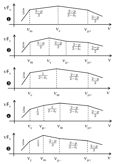
Figure 4: Generic synchrotron spectra in time decaying microturbulence with $-1<\alpha_{t}<0$, neglecting inverse Compton losses, with the spectral indices as indicated. Case 1: slow cooling scenario ($\gamma_{\rm c}>\gamma_{\rm m}$) with $t_{\rm dyn}<t_{\mu-}$, in which case the turbulence has not had time to relax to the background value $B_{\rm d}$; case 2: slow cooling scenario with $t_{\rm dyn}>t_{\mu-}$; case 3: fast cooling scenario with $\nu_{\mu-}<\nu_{\rm c}<\nu_{\rm m}$; case 4: fast cooling scenario with $\nu_{\rm c}<\nu_{\mu-}<\nu_{\rm m}$; case 5: fast cooling scenario with $\nu_{\rm c}<\nu_{\rm m}<\nu_{\mu-}$. See the discussion in Sec. A.1 for the precise definitions of the various frequencies and for modifications to these spectra if $\nu_{\rm c}$ or $\nu_{\rm m}$ exceeds $\nu_{\mu+}$, or if $\nu_{\rm max}$ is taken into account.

Depending on how $\nu_{\rm c}$, $\nu_{\rm m}$, $\nu_{\mu-}$ and $\nu_{\mu+}$ are ordered one relatively to each other, one obtains different synchrotron spectra. The various possible shapes of these spectra with their characteristic indices are summarized in the five cases depicted in Fig. 4 and the spectro-temporal indices of $F_{\nu}\propto t^{-\alpha}\nu^{-\beta}$ are provided in Table 1. This table assumes a decelerating blast wave in an external density profile $\propto r^{-k}$.

Table 1: Spectral ($\beta$) and temporal ($\alpha$) indices of $F_{\nu}\propto t^{-\alpha}\nu^{-\beta}$ for various orderings of the characteristic frequencies, assuming a decaying microturbulence with $-1<\alpha_{t}<0$, neglecting inverse Compton losses. The different spectra match those depicted in Fig. 4. Case 1: slow cooling, $t_{\rm dyn}<t_{\mu-}$; case 2: slow cooling, $t_{\rm dyn}>t_{\mu-}$; case 3: fast cooling scenario with $\nu_{\mu-}<\nu_{\rm c}<\nu_{\rm m}$; case 4: fast cooling scenario with $\nu_{\rm c}<\nu_{\mu-}<\nu_{\rm m}$; case 5: fast cooling scenario with $\nu_{\rm c}<\nu_{\rm m}<\nu_{\mu-}$. Note that the exact values of the characteristic frequencies vary from case to case, see the accompanying text for details. For all cases, $-\alpha=(2-3p)/4$ and $-\beta=-p/2$ if $\nu>\nu_{\mu+}$. The quantity $k$ refers to the external density profile $n\propto r^{-k}$.

Case	Frequency range	$-\beta$	$-\alpha$
Case 1	$\nu<\nu_{\rm m}$	$\frac{1}{3}$	$\frac{6(-2+k)+(-5+k)\alpha_{t}}{6(-4+k)}$
	$\nu_{\rm m}<\nu<\nu_{\rm c}$	$\frac{1-p}{2}$	$\frac{k(10-6p)+24(-1+p)+(-5+k)(1+p)\alpha_{t}}{8(-4+k)}$
	$\nu_{\rm c}<\nu<\nu_{\mu+}$	$\frac{-2p+(1-2p)\alpha_{t}}{4+3\alpha_{t}}$	$\frac{-2(-4+k)(-2+3p)+(-6+k(4-5p)+15p)\alpha_{t}}{2(-4+k)\left(4+3\alpha_{t}\right)}$
Case 2	$\nu<\nu_{\rm m}$	$\frac{1}{3}$	$\frac{2(-3+k)}{3(-4+k)}$
	$\nu_{\rm m}<\nu<\nu_{\rm c}$	$\frac{1-p}{2}$	$-\frac{(-3+k)(-1+p)}{-4+k}$
	$\nu_{\rm c}<\nu<\nu_{\mu-}$	$-\frac{p}{2}$	$\frac{-2+k+3p-kp}{-4+k}$
	$\nu_{\mu-}<\nu<\nu_{\mu+}$	$\frac{-2p+(1-2p)\alpha_{t}}{4+3\alpha_{t}}$	$\frac{-2(-4+k)(-2+3p)+(-6+k(4-5p)+15p)\alpha_{t}}{2(-4+k)\left(4+3\alpha_{t}\right)}$
Case 3	$\nu<\nu_{\rm c}$	$\frac{1}{3}$	$\frac{-4+6k+3(-5+k)\alpha_{t}}{6(-4+k)}$
	$\nu_{\rm c}<\nu<\nu_{\rm m}$	$-\frac{2+\alpha_{t}}{4+3\alpha_{t}}$	$-\frac{-8+2k+(-9+k)\alpha_{t}}{2(-4+k)\left(4+3\alpha_{t}\right)}$
	$\nu_{\rm m}<\nu<\nu_{\mu+}$	$\frac{-2p+(1-2p)\alpha_{t}}{4+3\alpha_{t}}$	$\frac{-2(-4+k)(-2+3p)+(-6+k(4-5p)+15p)\alpha_{t}}{2(-4+k)\left(4+3\alpha_{t}\right)}$
Case 4	$\nu<\nu_{\rm c}$	$\frac{1}{3}$	$\frac{2}{12-3k}$
	$\nu_{\rm c}<\nu<\nu_{\mu-}$	$-\frac{1}{2}$	$\frac{1}{-4+k}$
	$\nu_{\mu-}<\nu<\nu_{\rm m}$	$-\frac{2+\alpha_{t}}{4+3\alpha_{t}}$	$-\frac{-8+2k+(-9+k)\alpha_{t}}{2(-4+k)\left(4+3\alpha_{t}\right)}$
	$\nu_{\rm m}<\nu<\nu_{\mu+}$	$\frac{-2p+(1-2p)\alpha_{t}}{4+3\alpha_{t}}$	$\frac{-2(-4+k)(-2+3p)+(-6+k(4-5p)+15p)\alpha_{t}}{2(-4+k)\left(4+3\alpha_{t}\right)}$
Case 5	$\nu<\nu_{\rm c}$	$\frac{1}{3}$	$\frac{2}{12-3k}$
	$\nu_{\rm c}<\nu<\nu_{\rm m}$	$-\frac{1}{2}$	$\frac{1}{-4+k}$
	$\nu_{\rm m}<\nu<\nu_{\mu-}$	$-\frac{p}{2}$	$\frac{-2+k+3p-kp}{-4+k}$
	$\nu_{\mu-}<\nu<\nu_{\mu+}$	$\frac{-2p+(1-2p)\alpha_{t}}{4+3\alpha_{t}}$	$\frac{-2(-4+k)(-2+3p)+(-6+k(4-5p)+15p)\alpha_{t}}{2(-4+k)\left(4+3\alpha_{t}\right)}$

The following describes in some detail how the spectra are obtained, starting from the single particle spectra. Section A.3 discusses similar cases under the assumption of strong inverse Compton losses.

A.1.1 Fast cooling

Consider first the simplest case of fast cooling, for which $\nu_{\rm c}$ is smaller than all other critical frequencies. The quantity ${\rm d}P_{\nu}/{\rm d}\dot{N}_{e}$, see Eq. 40, represents the integral over the history of one cooling particle of initial Lorentz factor $\gamma_{\rm e,0}$.

If $\gamma_{e,0}>\gamma_{\mu+}$, the particle starts to cool in the undecayed part of the microturbulent layer where $\mu(t)<1$ and continues cooling in the decaying part, see Eq. 13. Straightforward integration of Eq. 40 then leads to $\nu\,{\rm d}P_{\nu}/{\rm d}\dot{N}_{e}\propto\nu^{1-b_{\nu}}$ with

$$1-b_{\nu}\,=\,\begin{cases}+1/2&\text{if}\,\,\nu_{\mu+}<\nu<\nu_{e,0,\delta B_{\mu}}\\ (1+\delta_{t}/2)/(2-\delta_{t})&\text{if}\,\,{\rm max}\left(\nu_{\mu-},\nu_{\rm c}\right)<\nu<\nu_{\mu+}\\ +1/2&\text{if}\,\,\nu_{\rm c}<\nu<\nu_{\mu-}\\ +4/3&\text{if}\,\,\nu<\nu_{\rm c}\\ \end{cases}$$ (59)

The frequency

$$\nu_{e,0,\delta B_{\mu}}\,\equiv\,\nu_{\rm p}\left[\gamma_{e,0};\delta B_{\mu}\right]\ .$$ (60)

Of course, the spectral power vanishes above $\nu_{e,0,\delta B_{\mu}}$.

If $\gamma_{e,0}<\gamma_{\mu+}$, which appears much more likely as discussed in Sec. 2.2, but $\gamma_{e,0}>\gamma_{\mu-}$ (and $\gamma_{e,0}>\gamma_{\rm c}$), then $\nu_{e,0}$ is obtained by solving first for the time $t_{e,0}$ at which the particle actually cools, as for $\nu_{\rm c}$ and $\nu_{\rm m}$:

$$t_{\rm syn}\left[\gamma_{e,0};\delta B\left(t_{e,0}\right)\right]=t_{e,0}\ ,$$ (61)

which leads to a shifted peak frequency

$$\nu_{e,0}=\nu_{e,0,\delta B_{\mu}}\left(\frac{\gamma_{e,0}}{\gamma_{\mu+}}\right)^{-\delta_{t}}\ .$$ (62)

Then

$$1-b_{\nu}\,=\,\begin{cases}2+2/\alpha_{t}&\text{if}\,\,\nu_{e,0}<\nu<\nu_{e,0,\delta B_{\mu}}\\ (1+\delta_{t}/2)(2-\delta_{t})&\text{if}\,\,{\rm max}\left(\nu_{\mu-},\nu_{\rm c}\right)<\nu<\nu_{e,0}\\ +1/2&\text{if}\,\,\nu_{\rm c}<\nu<\nu_{\mu-}\\ +4/3&\text{if}\,\,\nu<\nu_{\rm c}\\ \end{cases}$$ (63)

For $\nu_{e,0}<\nu<\nu_{e,0,\delta B_{\mu}}$, the standard index $+1/2$ has become $2+2/\alpha_{t}$, which may take large or small negative values depending on whether $\alpha_{t}$ lies close to 0 or to $-1$. This index corresponds to the radiation of a “non cooling” particle in a changing microturbulent magnetic field.

Finally, if $\gamma_{e,0}\ll\gamma_{\mu-}$ (but $\gamma_{e,0}\gg\gamma_{\rm c}$), the particle does not cool in the decaying microturbulence. The peak frequency for $\nu\,{\rm d}P_{\nu}/{\rm d}\dot{N}_{e}$ has moved to

$$\nu_{e,0}=\nu_{e,0,\delta B_{\mu}}\frac{B_{\rm d}}{\delta B_{\mu}}\ ,$$ (64)

as expected, and for $\nu_{e,0}<\nu<\nu_{e,0,\delta B_{\mu}}$, one finds the slope $2+2/\alpha_{t}$. Of course, for $\nu_{\rm c}<\nu<\nu_{e,0}$, one obtains $+1/2$.

Folding the previous results over the particle distribution of initial Lorentz factors is straightforward, albeit somewhat tedious. For the fast cooling scenario considered here, meaning $\nu_{\rm c}<\nu_{\rm m}$, this leads to three generic spectra depicted as cases $3$, $4$ and $5$ in Fig. 4, depending on the ordering of $\nu_{\rm c}$ and $\nu_{\rm m}$ relatively to $\nu_{\mu-}$: $\nu_{\mu-}<\nu_{\rm c}<\nu_{\rm m}$ (case 3), $\nu_{\rm c}<\nu_{\mu-}<\nu_{\rm m}$ (case 4), $\nu_{\rm c}<\nu_{\rm m}<\nu_{\mu-}$ (case 5). This figure does not consider the unlikely cases associated to the possibility $\nu_{\rm m}>\nu_{\mu+}$; these are briefly addressed further below. The distinctive features of these spectra can be summarized as follows.

If $\nu_{\mu-}<\nu_{\rm c}$, the slope of $\nu F_{\nu}$ becomes $+1/(2-\delta_{t})$ for $\nu_{\rm c}<\nu<\nu_{\rm m}$; if $\nu_{\rm c}<\nu_{\mu-}$ however, the slope is $+1/2$ for $\nu_{\rm c}<\nu<\nu_{\mu-}$ (fast cooling in $B_{\rm d}$) and $+1/(2-\delta_{t})$ for $\nu_{\mu-}<\nu<\nu_{\rm m}$ (fast cooling in decaying turbulence). For $\nu_{\rm m}<\nu<\nu_{\mu+}$, the slope is $(2-p)/(2-\delta_{t})$. The general trend of decaying microturbulence is to produce flatter synchrotron spectra than in a homogeneous magnetic field, due to the stretch in frequency associated to cooling in regions of different magnetic field strengths.

The maximal frequency $\nu_{\rm max}$ associated to $\gamma_{\rm max}$ is calculated in a similar fashion to $\nu_{\rm m}$. This frequency does not appear in Fig. 4 for the sake of clarity but its impact can be described as follows. If $\nu_{\rm max}>\nu_{\mu+}$, spectral power vanishes above $\nu_{\rm max}$. Otherwise, $\nu F_{\nu}$ has spectral index $2+2/\alpha_{t}$ for $\nu_{\rm max}<\nu<\nu_{\rm p}\left[\gamma_{\rm max};\delta B_{\mu}\right]$, which as before may take values close to zero if $\alpha_{t}$ is close to $-1$, and it vanishes beyond $\nu_{\rm p}\left[\gamma_{\rm max};\delta B_{\mu}\right]$.

The peak power $\nu F_{\nu}$ is radiated at $\nu_{\rm m}$ as usual, with

$$\left.\nu F_{\nu}\right|_{\nu=\nu_{\rm m}}\,\approx\,\frac{0.28}{4\pi D_{L}^{2}}\frac{4}{3}\gamma_{\rm b}^{2}\dot{N}_{e}\gamma_{\rm m}m_{e}c^{2}\ .$$ (65)

The above relates the maximum power to the incoming electron energy per unit time, which avoids specifying the value of the magnetic field in which cooling takes place. The numerical prefactor $0.28$ matches the prefactors derived in Panaitescu & Kumar (2000) for non-decaying turbulence, Lorentz beaming is included through the factor $4\gamma_{\rm b}^{2}/3$ and $\dot{N}_{e}$ has been defined in Eq. (16).

A.1.2 Slow cooling

For high energy particles with $\gamma_{e,0}>\gamma_{\rm c}$, the individual spectra of the quantity $\nu\,{\rm d}P_{\nu}/{\rm d}\dot{N}_{e}$ mimic those discussed in the fast cooling section before and this discussion thus concentrates on the bulk of electrons for which $\gamma_{e,0}<\gamma_{\rm c}$. Such electrons do not cool substantially anywhere in this slow cooling limit, therefore one finds either a slope $+4/3$ at low frequencies, or a slope $2+2/\alpha_{t}$ at high frequencies corresponding to the changing magnetic field. There are two frequencies associated to $\gamma_{e,0}$: $\nu_{e,0,\delta B_{\mu}}$ as before, corresponding to the peak frequency of emission when the particle experiences the undecayed $\delta B_{\mu}$, and $\nu_{e,0}$ the frequency to be calculated in the lowest magnetic field found downstream, i.e. at the back of the blast. Then

$$\nu_{e,0}\,=\,\nu_{\rm p}\left[\gamma_{e,0};\delta B_{\gamma_{\rm c}}\right]\ ,$$ (66)

provided $\gamma_{e,0}<\gamma_{\mu+}$.

As before, folding over the particle initial Lorentz distribution leads to the all-particle spectra. The possible spectra are displayed as cases $1$ and $2$ in Fig. 4, depending on the ordering of $t_{\rm dyn}$ vs $t_{\mu-}$: case $1$ if $t_{\rm dyn}<t_{\mu-}$, case 2 if $t_{\rm dyn}>t_{\mu-}$, which implies $\nu_{\rm c}<\nu_{\mu-}$ and $\delta B_{\gamma_{\rm c}}=B_{\rm d}$. If $\nu_{\rm c}>\nu_{\mu+}$, one would of course recover the spectrum of a standard slow cooling scenario in a homogeneous turbulence of strength $\delta B_{\mu}$.

The distinctive features of the $\nu F_{\nu}$ spectra can be summarized as follows: the slope $1-p/2$ of the fast cooling part of the particle population has been turned into $(2-p)/(2-\delta_{t})$ for ${\rm max}\left(\nu_{\rm c},\nu_{\mu-}\right)<\nu<\nu_{\mu+}$. The $+4/3$ slope for $\nu<\nu_{\rm m}$ remains unchanged, just as $(3-p)/2$ for $\nu_{\rm m}<\nu<\nu_{\rm c}$, or $1-p/2$ for $\nu_{\mu+}<\nu$ (assuming $\nu_{\mu+}<\nu_{\rm max}$ of course).

The peak power is now radiated at $\nu_{\rm c}$, with

$$\left.\nu F_{\nu}\right|_{\nu=\nu_{\rm c}}\,\approx\,\frac{0.28}{4\pi D_{L}^{2}}\frac{4}{3}\gamma_{\rm b}^{2}\dot{N}_{e}\gamma_{\rm c}m_{e}c^{2}\left(\frac{\gamma_{\rm c}}{\gamma_{\rm m}}\right)^{1-p}\ .$$ (67)

A.2 Rapid decay: $\alpha_{t}<-1$; no inverse Compton cooling

This Section now considers the limit in which the energy density stored in the microturbulence decreases faster than $t^{-1}$. Inverse Compton losses are neglected here; their impact is discussed in Sec. A.4. The crucial difference between the limit $\alpha_{t}<-1$ and that discussed in the previous Section has to do with the cooling history of a particle. In the present case, either the initial Lorentz factor $\gamma_{e,0}>\gamma_{\mu+}$, in which case the particle cools down to $\gamma_{\mu+}$ after crossing the undecayed part of the microturbulent layer, or $\gamma_{e,0}\leq\gamma_{\mu+}$, in which case it does not cool anywhere in the decaying microturbulent layer, see Eq. (13). In this latter case, the particle eventually cools in the background magnetic field, provided $t_{\rm dyn}>t_{\mu-}$.

The cooling Lorentz factor and its corresponding frequency should therefore be defined as follows. If $t_{\rm dyn}<t_{\mu+}$, one recovers a trivial case as it means that the turbulence has not relaxed beyond $\delta B_{\mu}$, hence the turbulence is homogeneous downstream. This case is not discussed further here. If $t_{\mu-}<t_{\rm dyn}$, the turbulence has relaxed to $B_{\rm d}$ by $t_{\rm dyn}$; in this case, $\gamma_{\rm c}$ is defined as usual in terms of $t_{\rm dyn}$ and $B_{\rm d}$. Indeed, cooling cannot take place in the decaying part of the microturbulent layer, but cooling is possible in the background shock compressed field $B_{\rm d}$. The cooling frequency then reads $\nu_{\rm c}=\nu_{\rm p}\left[\gamma_{\rm c};B_{\rm d}\right]$. In the intermediate limit, $t_{\mu+}<t_{\rm dyn}<t_{\mu-}$, the turbulence has not had time to relax down to $B_{\rm d}$. The cooling Lorentz factor remains undefined; however, one can understand the spectra obtained with the correspondence $\gamma_{\rm c}\rightarrow\gamma_{\mu+}$ and $\nu_{\rm c}\rightarrow\nu_{\mu+}$, since particles above $\gamma_{\mu+}$ do cool down to $\gamma_{\mu+}$ in $\delta B_{\mu}$.

For a particle of initial Lorentz factor $\gamma_{e,0}$, one should define two critical frequencies: $\nu_{e,0,\delta B_{\mu}}\equiv\nu_{\rm p}\left[\gamma_{e,0};\delta B_{\mu}\right]$ and $\nu_{e,0,B_{\rm d}}\equiv\nu_{\rm p}\left[\gamma_{e,0};B_{\rm d}\right]$. Note that the Lorentz factors $\gamma_{\mu+}$ and $\gamma_{\mu-}$ and their corresponding frequencies $\nu_{\mu+}$ and $\nu_{\mu-}$ remain unchanged here. It proves necessary to define a new frequency associated to particles of Lorentz factor $\gamma_{\mu+}$ radiating in the lowest magnetic field $\delta B_{\gamma_{\rm c}}$, with as before $\delta B_{\gamma_{\rm c}}\rightarrow B_{\rm d}$ if $t_{\rm dyn}>t_{\mu-}$:

$$\nu_{\mu 0}\,\equiv\,\nu_{\rm p}\left[\gamma_{\mu+};\,\delta B_{\gamma_{\rm c}}\right]\ .$$ (68)

One also define

$$\nu_{{\rm m},\delta B_{\mu}}\,=\,\nu_{\rm p}\left[\gamma_{\rm m};\,\delta B_{\mu}\right]\ .$$ (69)

The expression of the characteristic frequency $\nu_{\rm m}$ is given further below, case by case.

Spectra $\nu\,{\rm d}P_{\nu}/{\rm d}\dot{N}_{e}\propto\nu^{1-b_{\nu}}$ integrated over the cooling history of a particle of initial Lorentz factor $\gamma_{e,0}$ show:

$$1-b_{\nu}\,=\,\begin{cases}+1/2&\text{if}\,\,\nu_{\mu+}<\nu<\nu_{e,0,\delta B_{\mu}}\\ +1/2&\text{if}\,\,\nu_{\rm c}<\nu<\min\left(\nu_{\mu-},\nu_{e,0,B_{\rm d}}\right)\\ \min\left(2+2/\alpha_{t},\,4/3\right)&\text{if}\,\,\min\left(\nu_{\mu-},\nu_{e,0,B_{\rm d}}\right)<\nu\\ &\text{and}\,\,\nu<\min\left(\nu_{\mu+},\nu_{e,0,\delta B_{\mu}}\right)\\ \end{cases}$$ (70)

To understand the latter slope, one may recall that in a decaying microturbulence, radiation in a region of small extent but high magnetic power competes with radiation in a region of large extent at small magnetic power. If $\alpha_{t}<-3$, decay is so fast that most of the radiation is produced in $\delta B_{\mu}$ and one collects at low frequencies the $+4/3$ tail. If however, $-3<\alpha_{t}<-1$, the radiation produced by the particle as it crosses the decaying part of the turbulence dominates this tail and the slope becomes $2+2/\alpha_{t}$. This latter can be much flatter, possibly giving rise to a flat energy spectrum in the limit $\alpha_{t}\rightarrow-1$.

After folding over the particle population, one obtains the generic spectra depicted in Fig. 5 for $-3<\alpha_{t}<-4/(p+1)$ and in Fig. 6 for $-4/(p+1)<\alpha_{t}<-1$. The salient features of these spectra can be summarized as follows.

Consider for simplicity the limit $-3<\alpha_{t}<-4/(p+1)$. The other limit $-4/(p+1)<\alpha_{t}<-1$ can be understood in a similar way, while the limit $\alpha_{t}<-3$ follows from the former after replacing $2+2/\alpha_{t}$ with $4/3$. If $t_{\rm dyn}<t_{\mu-}$, the turbulence has not had time to relax down to $B_{\rm d}$. At high frequencies $>\nu_{{\rm m},\delta B_{\mu}}$, the spectrum then takes the form of a slow cooling scenario in a homogeneous turbulence of strength $\delta B_{\mu}$, with $\nu_{\rm c}\rightarrow\nu_{\mu+}$. As discussed above, the turbulence decays so fast that the early emission in the region of high magnetic power dominates that further away from the shock. At frequencies $\nu_{\rm m}<\nu<\nu_{{\rm m},\delta B_{\mu}}$, one collects the low energy extension with slope $2+2/\alpha_{t}$, instead of $4/3$ as discussed before. Note that the frequency $\nu_{\rm m}=\nu_{\rm p}\left[\gamma_{\rm m};\delta B_{\gamma_{\rm c}}\right]$. For $\nu<\nu_{\rm m}$, one recovers the slope $+4/3$ as expected. This case is denoted case 1 in Fig. 5.

In case 2, one now assumes $t_{\rm dyn}>t_{\mu-}$ (relaxed turbulence) and $\nu_{\rm c}>\nu_{\rm m}$ (slow cooling). The afterglow comprises two contributions: one associated to slow cooling in $\delta B_{\mu}$, as before; plus a second one associated to slow cooling in the background $B_{\rm d}$. This latter is indicated in dashed lines in Fig. 5; it exhibits a cut-off above $\nu_{\mu 0}$, since there are no particles with Lorentz factor above $\gamma_{\mu+}$ beyond $t_{\mu+}$. If $\gamma_{\rm max}<\gamma_{\mu+}$, the cut-off would of course take place at $\nu_{\rm p}\left[\gamma_{\rm max};B_{\rm d}\right]$. The characteristic frequency $\nu_{\rm m}=\nu_{\rm p}\left[\gamma_{\rm m};\,B_{\rm d}\right]$.

The peak power for the $\nu F_{\nu,B_{\rm d}}$ component associated to cooling in $B_{\rm d}$ is standard, while the power $\nu F_{\nu,\delta B_{\mu}}$ related to the decaying microturbulence can be written at $\nu_{\mu+}$ as

$$\left.\nu F_{\nu,\delta B_{\mu}}\right|_{\nu=\nu_{\mu+}}\,\approx\,\frac{0.28}{4\pi D_{L}^{2}}\frac{4}{3}\gamma_{\rm b}^{2}\dot{N}_{e}\gamma_{\mu+}m_{e}c^{2}\left(\frac{\gamma_{\mu+}}{\gamma_{\rm m}}\right)^{1-p}\ .$$ (71)

The ratio of energy fluxes at their respective peaks reads

$$\frac{\nu F_{\nu,B_{\rm d}}}{\nu F_{\nu,\delta B_{\mu}}}\,=\,\left(\frac{\gamma_{\rm c}}{\gamma_{\mu+}}\right)^{2-p}\,=\,\left(\frac{\delta B_{\mu}^{2}\,t_{\mu+}}{B_{\rm d}^{2}\,t_{\rm dyn}}\right)^{2-p}\ ,$$ (72)

and it scales as one would expect with the ratio of the product of synchrotron power times the exposure to the magnetic field.

One may also calculate the energy flux ratio at $\nu_{\rm m}$:

$$\frac{\nu_{\rm m}F_{\nu_{\rm m},B_{\rm d}}}{\nu_{\rm m}F_{\nu_{\rm m},\delta B_{\mu}}}\,=\,\frac{t_{\rm dyn}}{t_{\mu-}}\ .$$ (73)

In case 3, one now assumes a similar configuration with $t_{\rm dyn}>t_{\mu-}$ (relaxed turbulence), but $\nu_{\rm c}<\nu_{\rm m}$, meaning fast cooling in $B_{\rm d}$. The only difference with the previous spectrum corresponds to that change of cooling regime for the component $\nu F_{\nu,B_{\rm d}}$. As discussed before, the bulk of electrons cannot cool in the microturbulent field (as long as $\gamma_{\rm m}<\gamma_{\mu+}$).

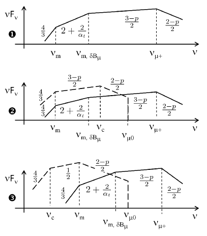
Figure 5: Generic synchrotron spectra in time decaying microturbulence with $-3<\alpha_{t}<-4/(p+1)$, neglecting inverse Compton losses, with the spectral indices as indicated. Case 1: scenario with $t_{\rm dyn}<t_{\mu-}$, in which case the turbulence has not had time to relax to the background value $B_{\rm d}$; case 2: slow cooling scenario with $t_{\rm dyn}>t_{\mu-}$; case 3: fast cooling scenario with $t_{\rm dyn}>t_{\mu-}$. See the discussion in Sec. A.2 for the precise definitions of the various frequencies. To obtain the spectra for $\alpha_{t}<-3$, it suffices to carry out the replacement $2+2/\alpha_{t}\rightarrow 4/3$. The dashed line represents the secondary synchrotron component associated to cooling in the background shock compressed field $B_{\rm d}$, whenever $t_{\rm dyn}>t_{\mu-}$.

Figure 6 shows the corresponding spectra for the case $-4/(p+1)<\alpha_{t}<-1$. The discussion is very similar to the previous one for $\alpha_{t}<-4/(p+1)$ and the differences are as follows. For $-4/(p+1)<\alpha_{t}<-1$, the spectral index $2+2/\alpha_{t}$ is softer than $(3-p)/2$; the low energy tail of index $2+2/\alpha_{t}$ of the high energy population thus extends from $\nu_{\mu+}$ down to $\nu_{\mu 0}$ as it dominates the slow cooling contribution of the bulk of electrons.

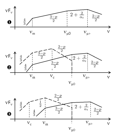
Figure 6: Same as Fig. 5 for $-4/(p+1)<\alpha_{t}<-1$.

The spectro-temporal indices of $F_{\nu}\propto t^{-\alpha}\nu^{-\beta}$ for these two values of $\alpha_{t}$ are provided in Table 2.

Table 2: Spectral ($\beta$) and temporal ($\alpha$) indices of $F_{\nu}\propto t^{-\alpha}\nu^{-\beta}$ assuming a decaying microturbulence with $-3<\alpha_{t}<-1$, with negligible inverse Compton losses. In cases 2 and 3, one must superimpose a synchrotron component associated to cooling in the background shock compressed magnetic field; the spectro-temporal slopes given here concern only the synchrotron component associated to the decaying microturbulent layer, not the latter. Case 1: $t_{\rm dyn}<t_{\mu-}$; case 2: $t_{\rm dyn}>t_{\mu-}$ with slow cooling in the background shock compressed field; case 3: $t_{\rm dyn}>t_{\mu-}$ with fast cooling in the background shock compressed field. The corresponding synchrotron spectra are shown in Fig. 5 for $-3<\alpha_{t}<\-4/(p+1)$ and in Fig. 6 for $-4/(p+1)<\alpha_{t}<-1$. For all cases, $-\alpha=(2-3p)/4$ and $-\beta=-p/2$ if $\nu>\nu_{\mu+}$. The quantity $k$ refers to the external density profile $n\propto r^{-k}$.

Case	Frequency range	$-\beta$	$-\alpha$
Case 1	$\nu<\nu_{\rm m}$	$\frac{1}{3}$	$\frac{6(-2+k)+(-5+k)\alpha_{t}}{6(-4+k)}$
$\left[-4/(p+1)<\alpha_{t}<-1\right]$	$\nu_{\rm m}<\nu<\nu_{\mu 0}$	$\frac{1-p}{2}$	$\frac{k(10-6p)+24(-1+p)+(-5+k)(1+p)\alpha_{t}}{8(-4+k)}$
	$\nu_{\mu 0}<\nu<\nu_{\mu+}$	$1+\frac{2}{\alpha_{t}}$	$\frac{2(6+k)+(2-k(-2+p)+9p)\alpha_{t}}{2(-4+k)\alpha_{t}}$
Cases 2 and 3	$\nu<\nu_{\rm m}$	$\frac{1}{3}$	$\frac{-6k+(3+k)\alpha_{t}}{6(-4+k)\alpha_{t}}$
$\left[-4/(p+1)<\alpha_{t}<-1\right]$	$\nu_{\rm m}<\nu<\nu_{\mu 0}$	$\frac{1-p}{2}$	$\frac{-2k+(-1+k+6p-2kp)\alpha_{t}}{2(-4+k)\alpha_{t}}$
	$\nu_{\mu 0}<\nu<\nu_{\mu+}$	$1+\frac{2}{\alpha_{t}}$	$\frac{2(6+k)+(2-k(-2+p)+9p)\alpha_{t}}{2(-4+k)\alpha_{t}}$
Case 1	$\nu<\nu_{\rm m}$	$\frac{1}{3}$	$\frac{6(-2+k)+(-5+k)\alpha_{t}}{6(-4+k)}$
$\left[-3<\alpha_{t}<-4/(p+1)\right]$	$\nu_{\rm m}<\nu<\nu_{{\rm m},\delta B_{\mu}}$	$1+\frac{2}{\alpha_{t}}$	$\frac{6(-4+k)+(-7+3k)\alpha_{t}}{2(-4+k)\alpha_{t}}$
	$\nu_{{\rm m},\delta B_{\mu}}<\nu<\nu_{\mu+}$	$\frac{1-p}{2}$	$\frac{2-3k-12p+3kp}{16-4k}$
Cases 2 and 3	$\nu<\nu_{\rm m}$	$\frac{1}{3}$	$\frac{-6k+(3+k)\alpha_{t}}{6(-4+k)\alpha_{t}}$
$\left[-3<\alpha_{t}<-4/(p+1)\right]$	$\nu_{\rm m}<\nu<\nu_{{\rm m},\delta B_{\mu}}$	$1+\frac{2}{\alpha_{t}}$	$\frac{6(-4+k)+(-7+3k)\alpha_{t}}{2(-4+k)\alpha_{t}}$
	$\nu_{{\rm m},\delta B_{\mu}}<\nu<\nu_{\mu+}$	$\frac{1-p}{2}$	$\frac{2-3k-12p+3kp}{16-4k}$

A.3 Gradual decay $\alpha_{t}>-4/(p+1)$, with dominant inverse Compton cooling

This Section assumes $-4/(p+1)<\alpha_{t}<0$ and it assumes that the Compton parameter $Y\gg 1$ for all Lorentz factors, everywhere in the blast. One defines

$$Y_{\mu}\equiv\frac{U_{\rm rad}}{\delta B_{\mu}^{2}/(8\pi)}\ ,$$ (74)

The cooling time of a particle is then defined as

$$t_{\rm cool}(\gamma_{e,0})\,\equiv\,\frac{1}{1+Y_{\mu}}t_{\rm syn}\left[\gamma_{e,0};\delta B_{\mu}\right]\ ,$$ (75)

and it is homogeneous throughout the blast. This simplifies the cooling history of a particle:

$$\gamma_{e}\,\simeq\,\begin{cases}\gamma_{e,0}&\text{if}\,\,t<t_{\rm cool}\left(\gamma_{e,0}\right)\\ \gamma_{e,0}\displaystyle{\frac{t_{\rm cool}\left(\gamma_{e,0}\right)}{t}}&\text{if}\,\,t>t_{\rm cool}\left(\gamma_{e,0}\right)\ .\end{cases}$$ (76)

The definitions of the critical Lorentz factors must be adapted to this case. One defines a Lorentz factor

$$\tilde{\gamma}_{\mu+}\,\equiv\,\frac{\gamma_{\mu+}}{1+Y_{\mu}}\ ,$$ (77)

such that inverse Compton cooling takes place at the end of the undecayed microturbulent layer. Similarly, one defines $\tilde{\gamma}_{\mu-}\equiv\tilde{\gamma}_{\mu+}t_{\mu+}/t_{\mu-}$. The associated frequency $\nu_{\mu+}$ (resp. $\nu_{\mu-}$) is defined as before in terms of $\tilde{\gamma}_{\mu+}$ (resp. $\tilde{\gamma}_{\mu-}$).

The cooling Lorentz factor is defined as

$$\tilde{\gamma}_{\rm c}=\tilde{\gamma}_{\mu+}\frac{t_{\mu+}}{t_{\rm dyn}}\ .$$ (78)

Eqs. 54,55 for the cooling frequency $\nu_{\rm c}$ and the definition of $\delta B_{\gamma_{\rm c}}$ remain valid. Regarding $\nu_{\rm m}$, Eq. 57 remains valid but the definition of $\delta B_{\gamma_{\rm m}}$ must be modified to account for inverse Compton losses:

$$\delta B_{\gamma_{\rm m}}\,=\,\max\left\{\delta B_{\gamma_{\rm c}},\,\delta B_{\mu}\left(\frac{\gamma_{\rm m}}{\tilde{\gamma}_{\mu+}}\right)^{-\alpha_{t}/2}\right\}\ .$$ (79)

The index of $\nu\,{\rm d}P_{\nu}/{\rm d}\dot{N}_{e}$ differs from the standard case of homogeneous turbulence only if the particle radiates in the changing magnetic field while it is cooling in the radiation field. This applies to the spectral domain ${\rm max}\left(\nu_{\mu-},\nu_{\rm c}\right)<\nu<{\rm min}\left(\nu_{e,0},\nu_{\mu+}\right)$, in which the index of $\nu\,{\rm d}P_{\nu}/{\rm d}\dot{N}_{e}$ becomes $(1-\alpha_{t})/(2-\alpha_{t}/2)$. The frequency $\nu_{e,0}$ is defined in terms of $\gamma_{e,0}$ as $\nu_{\rm m}$ in terms of $\gamma_{\rm m}$.

After folding over the particle Lorentz distribution, one obtains the generic full all-particle spectra represented in Fig. 7. As before, this figure ignores a possible maximal frequency $\nu_{\rm max}$ and assumes that $\nu_{\rm c}$ and $\nu_{\rm m}$ are smaller than $\nu_{\mu+}$. The discussion is very similar to that given in Sec. A.1 and is not be repeated here. The significant differences lie in the spectral indices: $(2-p)/(2-\delta_{t})$ has become $(2-p-\alpha_{t})/(2-\alpha_{t}/2)$, while $1/(2-\delta_{t})$ (otherwise $1/2$ for standard fast cooling) has become $(1-\alpha_{t})/(2-\alpha_{t}/2)$. Inverse Compton losses take away a large fraction of the dissipated energy, so that the synchrotron peak power is modified as follows, for slow cooling (cases 1 and 2):

$$\left.\nu F_{\nu}\right|_{\nu=\nu_{\rm c}} \,\approx\, \frac{0.28}{4\pi D_{L}^{2}}\frac{4}{3}\gamma_{\rm b}^{2}\dot{N}_{e}\gamma_{\rm c}m_{e}c^{2}\left(\frac{\tilde{\gamma}_{\rm c}}{\gamma_{\rm m}}\right)^{1-p}\times$$ (80)

$$\quad\quad\frac{1}{1+Y_{\mu}}\frac{\delta B_{\gamma_{\rm c}}^{2}}{\delta B_{\mu}^{2}}\ .$$

and for fast cooling (cases 3, 4 and 5):

$$\left.\nu F_{\nu}\right|_{\nu=\nu_{\rm m}} \,\approx\, \frac{0.28}{4\pi D_{L}^{2}}\frac{4}{3}\gamma_{\rm b}^{2}\dot{N}_{e}\gamma_{\rm m}m_{e}c^{2}\times$$ (81)

$$\quad\quad\frac{1}{1+Y_{\mu}}\frac{\delta B_{\gamma_{\rm m}}^{2}}{\delta B_{\mu}^{2}}\ .$$

The ratios of magnetic energy densities $\delta B_{\gamma_{\rm c}}^{2}/\delta B_{\mu}^{2}$ (resp. $\delta B_{\gamma_{\rm m}}^{2}/\delta B_{\mu}^{2}$) that appear in the both expressions, yield the proper $Y$ Compton parameter at the location at which most of the cooling of particles of Lorentz factor $\gamma_{\rm c}$ (resp. $\gamma_{\rm m}$) occurs.

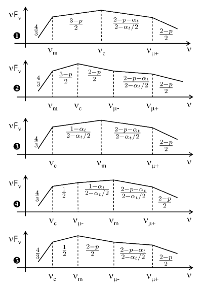
Figure 7: Generic synchrotron spectra in time decaying microturbulence with $-4/(p+1)<\alpha_{t}<0$, assuming that inverse Compton losses dominate over synchrotron losses everywhere in the blast. Case 1: slow cooling scenario ($\gamma_{\rm c}>\gamma_{\rm m}$) with $t_{\rm dyn}<t_{\mu-}$, in which case the turbulence has not had time to relax to the background value $B_{\rm d}$; case 2: slow cooling scenario with $t_{\rm dyn}>t_{\mu-}$; case 3: fast cooling scenario with $\nu_{\mu-}<\nu_{\rm c}<\nu_{\rm m}$; case 4: fast cooling scenario with $\nu_{\rm c}<\nu_{\mu-}<\nu_{\rm m}$; case 5: fast cooling scenario with $\nu_{\rm c}<\nu_{\rm min}<\nu_{\mu-}$. See the discussion in Sec. A.3 for the precise definitions of the various frequencies and for modifications to these spectra if $\nu_{\rm c}$ or $\nu_{\rm m}$ exceeds $\nu_{\mu+}$, or if $\nu_{\rm max}$ is taken into account. Note that the spectral slope $(2-p-\alpha_{t})/(2-\alpha_{t}/2)$ takes positive values whenever $\alpha_{t}<2-p$.

The corresponding spectro-temporal indices for $F_{\nu}\propto t^{-\alpha}\nu^{-\beta}$ are given in Table 3.

Table 3: Spectral ($\beta$) and temporal ($\alpha$) indices of $F_{\nu}\propto t^{-\alpha}\nu^{-\beta}$ for various orderings of the characteristic frequencies, assuming a decaying microturbulence with $-4/(p+1)<\alpha_{t}$, with dominant inverse Compton losses everywhere in the blast. Case 1: slow cooling with $t_{\rm dyn}<t_{\mu-}$; case 2: slow cooling with $t_{\rm dyn}>t_{\mu-}$; case 3: fast cooling scenario with $\nu_{\mu-}<\nu_{\rm c}<\nu_{\rm m}$; case 4: fast cooling scenario with $\nu_{\rm c}<\nu_{\mu-}<\nu_{\rm m}$; case 5: fast cooling scenario with $\nu_{\rm c}<\nu_{\rm min}<\nu_{\mu-}$. The corresponding synchrotron spectra are shown in Fig. 7. For all cases, $-\alpha=(2-3p)/4$ and $-\beta=-p/2$ if $\nu>\nu_{\mu+}$. The quantity $k$ refers to the external density profile $n\propto r^{-k}$.

Case	Frequency range	$-\beta$	$-\alpha$
Case 1	$\nu<\nu_{\rm m}$	$\frac{1}{3}$	$\frac{6(-2+k)+(-5+k)\alpha_{t}}{6(-4+k)}$
	$\nu_{\rm m}<\nu<\nu_{\rm c}$	$\frac{1-p}{2}$	$\frac{k(10-6p)+24(-1+p)+(-5+k)(1+p)\alpha_{t}}{8(-4+k)}$
	$\nu_{\rm c}<\nu<\nu_{\mu+}$	$\frac{2p+\alpha_{t}}{-4+\alpha_{t}}$	$\frac{2(-4+k)(-2+3p)+(2-k(-2+p)+9p)\alpha_{t}}{2(-4+k)\left(-4+\alpha_{t}\right)}$
Case 2	$\nu<\nu_{\rm m}$	$\frac{1}{3}$	$\frac{2(-3+k)}{3(-4+k)}$
	$\nu_{\rm m}<\nu<\nu_{\rm c}$	$\frac{1-p}{2}$	$-\frac{(-3+k)(-1+p)}{-4+k}$
	$\nu_{\rm c}<\nu<\nu_{\mu-}$	$-\frac{p}{2}$	$-\frac{2+(-3+k)p}{-4+k}$
	$\nu_{\mu-}<\nu<\nu_{\mu+}$	$\frac{2p+\alpha_{t}}{-4+\alpha_{t}}$	$\frac{2(-4+k)(-2+3p)+(2-k(-2+p)+9p)\alpha_{t}}{2(-4+k)\left(-4+\alpha_{t}\right)}$
Case 3	$\nu<\nu_{\rm c}$	$\frac{1}{3}$	$\frac{-4+6k+(-5+k)\alpha_{t}}{6(-4+k)}$
	$\nu_{\rm c}<\nu<\nu_{\rm m}$	$\frac{2+\alpha_{t}}{-4+\alpha_{t}}$	$\frac{2(-4+k)+(11+k)\alpha_{t}}{2(-4+k)\left(-4+\alpha_{t}\right)}$
	$\nu_{\rm m}<\nu<\nu_{\mu+}$	$\frac{2p+\alpha_{t}}{-4+\alpha_{t}}$	$\frac{2(-4+k)(-2+3p)+(2-k(-2+p)+9p)\alpha_{t}}{2(-4+k)\left(-4+\alpha_{t}\right)}$
Case 4	$\nu<\nu_{\rm c}$	$\frac{1}{3}$	$\frac{2(-1+k)}{3(-4+k)}$
	$\nu_{\rm c}<\nu<\nu_{\mu-}$	$-\frac{1}{2}$	$\frac{1-k}{-4+k}$
	$\nu_{\mu-}<\nu<\nu_{\rm m}$	$\frac{2+\alpha_{t}}{-4+\alpha_{t}}$	$\frac{2(-4+k)+(11+k)\alpha_{t}}{2(-4+k)\left(-4+\alpha_{t}\right)}$
	$\nu_{\rm m}<\nu<\nu_{\mu+}$	$\frac{2p+\alpha_{t}}{-4+\alpha_{t}}$	$\frac{2(-4+k)(-2+3p)+(2-k(-2+p)+9p)\alpha_{t}}{2(-4+k)\left(-4+\alpha_{t}\right)}$
Case 5	$\nu<\nu_{\rm c}$	$\frac{1}{3}$	$\frac{2(-1+k)}{3(-4+k)}$
	$\nu_{\rm c}<\nu<\nu_{\rm m}$	$-\frac{1}{2}$	$\frac{1-k}{-4+k}$
	$\nu_{\rm m}<\nu<\nu_{\mu-}$	$-\frac{p}{2}$	$-\frac{2+(-3+k)p}{-4+k}$
	$\nu_{\mu-}<\nu<\nu_{\mu+}$	$\frac{2p+\alpha_{t}}{-4+\alpha_{t}}$	$\frac{2(-4+k)(-2+3p)+(2-k(-2+p)+9p)\alpha_{t}}{2(-4+k)\left(-4+\alpha_{t}\right)}$

A.4 Rapid decay $-3<\alpha_{t}<-4/(p+1)$, with dominant inverse Compton cooling

Finally, one must consider the possibility that $-3<\alpha_{t}<-4/(p+1)$ with dominant inverse Compton losses, as in the previous Section A.3. The generic spectra obtained after folding over the particle population are depicted in Fig. 8. The critical frequencies are defined as in the previous Section A.3.

The characteristic features of these spectra mix those of Sec. A.3 [gradual decay, $\alpha_{t}>-4/(p+1)$ with inverse Compton losses] with those of Sec. A.2 (rapid decay, $\alpha_{t}<-1$, no inverse Compton losses). They can be summarized and understood as follows.

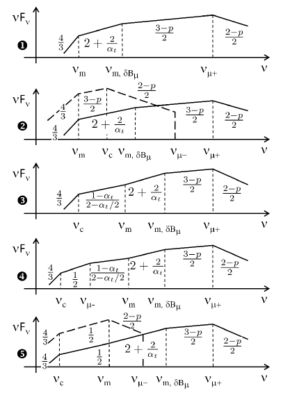
Figure 8: Generic synchrotron spectra in time decaying microturbulence with $-3<\alpha_{t}<-4/(p+1)$, assuming that inverse Compton losses dominate throughout the blast. The spectral indices as indicated. Case 1: slow cooling scenario with $t_{\rm dyn}<t_{\mu-}$, in which case the turbulence has not had time to relax to the background value $B_{\rm d}$; case 2: slow cooling scenario with $t_{\rm dyn}>t_{\mu-}$; case 3: fast cooling scenario with $\nu_{\mu-}<\nu_{\rm c}<\nu_{\rm m}$; case 4: fast cooling scenario with $\nu_{\rm c}<\nu_{\mu-}<\nu_{\rm m}$; case 5: fast cooling scenario with $\nu_{\rm c}<\nu_{\rm m}<\nu_{\mu-}$. See the discussion in Sec. A.4 for the precise definitions of the various frequencies and for modifications to these spectra if $\nu_{\rm c}$ or $\nu_{\rm m}$ exceeds $\nu_{\mu+}$, or if $\nu_{\rm max}$ is taken into account. The dashed line represents the secondary synchrotron component associated to cooling in the background shock compressed field $B_{\rm d}$ as in Fig. 5.

Cases 1 and 2 depict a slow cooling scenario $\gamma_{\rm m}<\tilde{\gamma}_{\rm c}$ with either $t_{\rm dyn}<t_{\mu-}$ (case 1) or $t_{\rm dyn}>t_{\mu-}$ (case 2). Because the bulk of electrons do not actually cool, the spectra obtained match those of cases 1 and 2 in Fig. 5, for which inverse Compton losses are absent.

Cases 3 and 4 depict fast cooling regimes with different orderings of $\nu_{\rm c}$ relatively to $\nu_{\mu-}$, but $\nu_{\rm m}>\nu_{\mu-}$. The peak power still occurs at $\nu_{\mu+}$ due to the rapid decay of the microturbulence and the spectra keep a shape similar to those of cases 1 and 2, up to the fast decaying index at low frequencies $\nu_{\rm c}<\nu<\nu_{\rm m}$. Case 4 differs somewhat from its counterpart when inverse Compton losses are neglected, which is represented as case 3 in Fig. 5, because it does not reveal an additional synchrotron fast cooling component in the background shock compressed magnetic field. This absence is directly related to the presence of inverse Compton losses, which cut the electron distribution down to $\gamma_{\mu-}<\gamma_{\rm m}$ by the end of the microturbulent layer, so that the electron distribution is mostly monoenergetic at that point and cooling in the background magnetic field ensues with generic slope $1/2$.

In contrast, $\gamma_{\rm m}<\gamma_{\mu-}$ in case 5. Then the electron distribution maintains a powerlaw shape between $\gamma_{\rm m}$ and $\gamma_{\mu-}$ at the end of the microturbulence layer, so that an additional component associated to cooling in the background field emerges, as shown in Fig. 8.

The corresponding spectro-temporal indices for $F_{\nu}\propto t^{-\alpha}\nu^{\beta}$ are given in Table 4.

The peak power for the synchrotron component associated to the microturbulent layer occurs at $\nu_{\mu+}$ in all cases with

$$\left.\nu F_{\nu,\delta B_{\mu}}\right|_{\nu=\nu_{\mu+}}\,\approx\,\frac{0.28}{4\pi D_{L}^{2}}\frac{4}{3}\gamma_{\rm b}^{2}\dot{N}_{e}\frac{\tilde{\gamma}_{\mu+}}{1+Y_{\mu}}m_{e}c^{2}\left(\frac{\tilde{\gamma}_{\mu+}}{\gamma_{\rm m}}\right)^{1-p}\ .$$ (82)

The ratio between the peak powers of each synchrotron component for case 5 reads

$$\frac{\nu F_{\nu,B_{\rm d}}}{\nu F_{\nu,\delta B_{\mu}}}\,=\,\left(\frac{\gamma_{\rm m}}{\tilde{\gamma}_{\mu+}}\right)^{2-p}\frac{B_{\rm d}^{2}}{\delta B_{\mu}^{2}}\ ,$$ (83)

which resembles Eq. 83 up to an additional factor $B_{\rm d}^{2}/\delta B_{\mu}^{2}$ at the benefit of the high energy microturbulent component, due to the competition between synchrotron and inverse Compton losses.

Table 4: Spectral ($\beta$) and temporal ($\alpha$) indices of $F_{\nu}\propto t^{-\alpha}\nu^{-\beta}$ for various orderings of the characteristic frequencies, assuming a decaying microturbulence with $-3<\alpha_{t}<-4/(p+1)$, with dominant inverse Compton losses everywhere in the blast. In case 2 and 5, one must superimpose a synchrotron component associated to cooling in the background shock compressed magnetic field; the spectro-temporal slopes given here concern only the synchrotron component associated to the decaying microturbulent layer, not the latter. Case 1: slow cooling with $t_{\rm dyn}<t_{\mu-}$; case 2: slow cooling scenario with $t_{\rm dyn}>t_{\mu-}$; case 3: fast cooling scenario with $\nu_{\mu-}<\nu_{\rm c}<\nu_{\rm m}$; case 4: fast cooling scenario with $\nu_{\rm c}<\nu_{\mu-}<\nu_{\rm m}$; case 5: fast cooling scenario with $\nu_{\rm c}<\nu_{\rm min}<\nu_{\mu-}$. The corresponding synchrotron spectra are shown in Fig. 8. For all cases, $-\alpha=(2-3p)/4$ and $-\beta=-p/2$ if $\nu>\nu_{\mu+}$. The quantity $k$ refers to the external density profile $n\propto r^{-k}$.

Case	Frequency range	$-\beta$	$-\alpha$
Case 1	$\nu<\nu_{\rm m}$	$\frac{1}{3}$	$\frac{6(-2+k)+(-5+k)\alpha_{t}}{6(-4+k)}$
	$\nu_{\rm m}<\nu<\nu_{{\rm m},\delta B_{\mu}}$	$1+\frac{2}{\alpha_{t}}$	$\frac{6(-4+k)+(-7+3k)\alpha_{t}}{2(-4+k)\alpha_{t}}$
	$\nu_{{\rm m},\delta B_{\mu}}<\nu<\nu_{\mu+}$	$\frac{1-p}{2}$	$\frac{2-3k-12p+3kp}{16-4k}$
Case 2	$\nu<\nu_{\rm m}$	$\frac{1}{3}$	$\frac{-6k+(3+k)\alpha_{t}}{6(-4+k)\alpha_{t}}$
	$\nu_{\rm m}<\nu<\nu_{{\rm m},\delta B_{\mu}}$	$1+\frac{2}{\alpha_{t}}$	$\frac{6(-4+k)+(-7+3k)\alpha_{t}}{2(-4+k)\alpha_{t}}$
	$\nu_{{\rm m},\delta B_{\mu}}<\nu<\nu_{\mu+}$	$\frac{1-p}{2}$	$\frac{2-3k-12p+3kp}{16-4k}$
Case 3	$\nu<\nu_{\rm c}$	$\frac{1}{3}$	$\frac{-4+6k+(-5+k)\alpha_{t}}{6(-4+k)}$
	$\nu_{\rm c}<\nu<\nu_{\rm m}$	$\frac{2+\alpha_{t}}{-4+\alpha_{t}}$	$\frac{2(-4+k)+(11+k)\alpha_{t}}{2(-4+k)\left(-4+\alpha_{t}\right)}$
	$\nu_{\rm m}<\nu<\nu_{{\rm m},\delta B_{\mu}}$	$1+\frac{2}{\alpha_{t}}$	$\frac{6(-4+k)+(-7+3k)\alpha_{t}}{2(-4+k)\alpha_{t}}$
	$\nu_{{\rm m},\delta B_{\mu}}<\nu<\nu_{\mu+}$	$\frac{1-p}{2}$	$\frac{2-3k-12p+3kp}{16-4k}$
Case 4	$\nu<\nu_{\rm c}$	$\frac{1}{3}$	$\frac{-16+6k-5(-5+k)\alpha_{t}}{24(-4+k)}$
	$\nu_{\rm c}<\nu<\nu_{\mu-}$	$-\frac{1}{2}$	$\frac{1-k}{-4+k}$
	$\nu_{\mu-}<\nu<\nu_{\rm m}$	$\frac{2+\alpha_{t}}{-4+\alpha_{t}}$	$\frac{2(-4+k)+(11+k)\alpha_{t}}{2(-4+k)\left(-4+\alpha_{t}\right)}$
	$\nu_{\rm m}<\nu<\nu_{{\rm m},\delta B_{\mu}}$	$1+\frac{2}{\alpha_{t}}$	$\frac{6(-4+k)+(-7+3k)\alpha_{t}}{2(-4+k)\alpha_{t}}$
	$\nu_{{\rm m},\delta B_{\mu}}<\nu<\nu_{\mu+}$	$\frac{1-p}{2}$	$\frac{2-3k-12p+3kp}{16-4k}$
Case 5	$\nu<\nu_{\rm c}$	$\frac{1}{3}$	$\frac{-6k+(23+k)\alpha_{t}}{6(-4+k)\alpha_{t}}$
	$\nu_{\rm c}<\nu<\nu_{\rm m}$	$-\frac{1}{2}$	$\frac{-2k+(11-3k)\alpha_{t}}{2(-4+k)\alpha_{t}}$
	$\nu_{\rm m}<\nu<\nu_{{\rm m},\delta B_{\mu}}$	$1+\frac{2}{\alpha_{t}}$	$\frac{6(-4+k)+(-7+3k)\alpha_{t}}{2(-4+k)\alpha_{t}}$
	$\nu_{{\rm m},\delta B_{\mu}}<\nu<\nu_{\mu+}$	$\frac{1-p}{2}$	$\frac{2-3k-12p+3kp}{16-4k}$

A.5 Synchrotron self-absorption

At very low frequencies, the synchrotron spectrum may be modified by opacity effects. The absorption break frequency generally lies well below the optical domain, e.g. for a homogeneous turbulence, $k=0$ (constant density profile) and a slow cooling regime, one finds $\nu_{\rm abs}\sim 3\times 10^{7}\,{\rm Hz}\,E_{53}^{1/5}n_{-3}^{3/5}\epsilon_{B,-2}^{1/5}\epsilon_{e,-0.3}^{-1}z_{+,0.3}^{-1}$ (see Panaitescu & Kumar 2000). In this standard case, the frequency index of $F_{\nu}$ is $2$ below the absorption frequency, e.g. Granot et al. (1999) and references therein.

Accounting for the decaying microturbulence modifies the situation as follows. All calculations are performed in the comoving downstream frame, as indicated by the primes. Moreover, the self-similar profile of the blast and the secular evolution of the blast characteristics are neglected, as in the rest of App. A. One then defines the synchrotron self-absorption coefficient (Rybicki & Lightman, 1979):

$$\alpha^{\prime}_{\nu^{\prime}}\,=\,-\frac{1}{8\pi m_{e}\nu^{\prime 2}}\,\int{\rm d}\gamma_{e}\,P^{\prime}_{\nu^{\prime}/e}\gamma_{e}^{2}\frac{\partial}{\partial\gamma_{e}}\left(\frac{1}{\gamma_{e}^{2}}\frac{{\rm d}n^{\prime}}{{\rm d}\gamma_{e}}\right)\ ,$$ (84)

with $P^{\prime}_{\nu^{\prime}/e}\,\equiv\,{\rm d}E/{\rm d}\nu^{\prime}{\rm d}t^{\prime}$ the spectral synchrotron power emitted per electron per frequency interval, as defined in Eq. 43 up to the change of frame for the frequency. Here however, one considers only the low frequency part $\propto\nu^{1/3}$ since one is interested in frequencies well below $\nu_{\rm m}$. The electron distribution function ${\rm d}n^{\prime}/{\rm d}\gamma_{e}$ depends on the distance to the shock front when cooling is efficient. Since only the minimum Lorentz factor is of importance in the calculations of synchrotron self-absorption, one can approximate the distribution as a unique powerlaw,

$$\frac{{\rm d}n^{\prime}}{{\rm d}\gamma_{e}}\,=\,\frac{1}{\gamma_{i}}\left(\frac{\gamma_{e}}{\gamma_{i}}\right)^{-q}n^{\prime}(q-1)$$ (85)

with $\gamma_{i}=\gamma_{\rm m}$ at distances such that cooling is inefficient for particles of Lorentz factor $\gamma_{\rm m}$, and $\gamma_{i}$ position dependent at larger distances from the shock front. Of course, in a slow cooling regime, $\gamma_{i}=\gamma_{\rm m}$ everywhere in the blast. The index $q$ departs from $s$ only when cooling becomes efficient; its exact value does not affect the following up to factors of order unity. The above integral leads to

$$\alpha^{\prime}_{\nu^{\prime}}\,\simeq\,5\frac{en^{\prime}}{\delta B}\gamma_{i}^{-5}\left(\frac{\nu^{\prime}}{\nu^{\prime}_{i}}\right)^{-5/3}\ ,$$ (86)

with $\nu^{\prime}_{i}\equiv\nu_{\rm p}^{\prime}\left[\delta B;\gamma_{i}\right]$. This local absorption coefficient depends on position both through $\gamma_{i}$ (when cooling is efficient) and through $\delta B$, in the presence of decaying turbulence. One may thus rewrite the absorption coefficient as

$$\alpha^{\prime}_{\nu^{\prime}}\,\simeq\,\alpha^{\prime}_{\mu,\nu^{\prime}}\left(\frac{\delta B}{\delta B_{\mu}}\right)^{2/3}\left(\frac{\gamma_{i}}{\gamma_{\rm m}}\right)^{-5/3}\ ,$$ (87)

with $\alpha^{\prime}_{\mu,\nu^{\prime}}$ the absorption coefficient defined according to Eq. 86 with $\delta B\rightarrow\delta B_{\mu}$ and $\gamma_{i}\rightarrow\gamma_{\rm m}$. This formulation allows to write $\alpha^{\prime}_{\nu^{\prime}}$ as a broken power law function of the distance to the shock front.

The emission coefficient $j^{\prime}_{\nu^{\prime}}$ is defined as

$$j^{\prime}_{\nu^{\prime}}=\frac{1}{4\pi}\int{\rm d}\gamma_{e}\,P^{\prime}_{\nu^{\prime}/e}\frac{{\rm d}n^{\prime}}{{\rm d}\gamma_{e}}\ ,$$ (88)

assuming isotropic emission, and it can be recast similarly to $\alpha^{\prime}_{\nu^{\prime}}$ into

$$j^{\prime}_{\nu^{\prime}}\,=\,j^{\prime}_{\mu,\nu^{\prime}}\left(\frac{\delta B}{\delta B_{\mu}}\right)^{2/3}\left(\frac{\gamma_{i}}{\gamma_{\rm m}}\right)^{-2/3}\ ,$$ (89)

with $j^{\prime}_{\mu,\nu^{\prime}}\,\simeq\,0.4e^{3}\delta B_{\mu}(m_{e}c^{2})^{-1}n^{\prime}\left(\nu^{\prime}/\nu^{\prime}_{\mu,\rm m}\right)^{1/3}$ and $\nu^{\prime}_{\mu,\rm m}\equiv\nu_{\rm p}^{\prime}\left[\delta B_{\mu};\gamma_{\rm m}\right]$.

The specific intensity along a ray path obeys the radiative transfer equation

$$\frac{{\rm d}I^{\prime}_{\nu^{\prime}}}{{\rm d}s}\,=\,-\alpha^{\prime}_{\nu^{\prime}}I^{\prime}_{\nu^{\prime}}+j^{\prime}_{\nu^{\prime}}\ ,$$ (90)

with the usual formal solution

$$I^{\prime}_{\nu^{\prime}}(x=0)\,=\,\int_{0}^{\tau_{\nu^{\prime},\rm b}}\frac{j^{\prime}_{\nu^{\prime}}}{\alpha^{\prime}_{\nu^{\prime}}}\,e^{-\tau_{\nu^{\prime}}}\,{\rm d}\tau_{\nu^{\prime}}\ .$$ (91)

Here ${\rm d}\tau_{\nu^{\prime}}=\alpha^{\prime}_{\nu^{\prime}}{\rm d}x$, $x>0$ denotes the distance from the shock front, and $\tau_{\nu^{\prime}}(x=0)\equiv 0$ by convention. The parameter $\tau_{\nu^{\prime},\rm b}$ consequently represents the total optical depth of the blast which can be derived by integrating the broken power law form of Eq. 87 over $x$, from $x=0$ up to $x_{\rm b}\sim r/\gamma_{\rm b}\sim t_{\rm dyn}/c$. The above formulation of the solution of the equation of radiative transfer is particularly appealing because it leads to a simple evaluation of $I^{\prime}_{\nu^{\prime}}(0)$ in various cases.

In particular, if the regime is slow cooling, $\gamma_{i}=\gamma_{\rm m}$ everywhere and $j^{\prime}_{\nu^{\prime}}/\alpha^{\prime}_{\nu^{\prime}}$ becomes uniform in the blast, as in the homogeneous (slow cooling) case. Then one finds

$$I^{\prime}_{\nu^{\prime}}(0)=\frac{j^{\prime}_{\mu,\nu^{\prime}}}{\alpha^{\prime}_{\mu,\nu^{\prime}}}\left(1-e^{-\tau_{\nu^{\prime},\rm b}}\right)\ .$$ (92)

In the optically thick limit $\tau_{\nu^{\prime},\rm b}\gg 1$, the ratio $j^{\prime}_{\mu,\nu^{\prime}}/\alpha^{\prime}_{\mu,\nu^{\prime}}$ leads to the standard slope $2$ for $F_{\nu}$ below the absorption frequency $\nu^{\prime}_{\rm abs,b}$, which is defined by the condition $\tau_{\nu^{\prime},\rm b}=1$ at $\nu^{\prime}_{\rm abs,b}$. Note that $\tau_{\nu^{\prime},\rm b}$ shares with the absorption coefficient $\alpha^{\prime}_{\nu^{\prime}}$ the scaling $\propto\nu^{\prime-5/3}$. In the optically thin limit $\tau_{\nu^{\prime},\rm b}\ll 1$, meaning $\nu^{\prime}\gg\nu^{\prime}_{\rm abs,b}$, one recovers the slope $1/3$ since $\tau_{\nu^{\prime},\rm b}\propto\alpha^{\prime}_{\mu,\nu^{\prime}}$. The non trivial dependence of $\nu^{\prime}_{\rm abs,b}$ on time leads to a non trivial time dependence of the flux below the break frequency. This dependence is not discussed here, but can be calculated through $\tau_{\nu^{\prime},\rm b}$.

The fast cooling regime leads to a more complicated shape of the spectrum in the transition region between the asymptotic thin and thick regimes (for a similar discussion with a homogeneous turbulence, see Granot et al. 2000). One needs to define here an intermediate optical depth,

$$\tau_{\nu^{\prime},\rm m}=\int_{0}^{x_{\rm cool,m}}\alpha^{\prime}_{\nu^{\prime}}\,{\rm d}x\ ,$$ (93)

with $x_{\rm cool,m}$ the location at which particles of Lorentz factor $\gamma_{\rm m}$ start to cool. The fast cooling regime implies that by the back of the blast, such particles have cooled down to $\gamma_{\rm c}$. One now defines an absorption frequency $\nu^{\prime}_{\rm abs,m}$ such that $\tau_{\nu^{\prime},\rm m}=1$ at $\nu^{\prime}_{\rm abs,m}$. Because the optical depth is an increasing function of distance to the shock front, $\tau_{\nu^{\prime},\rm m}<\tau_{\nu^{\prime},\rm b}$ (possibly $\tau_{\nu^{\prime},\rm m}\ll\tau_{\nu^{\prime},\rm b}$) and $\nu^{\prime}_{\rm abs,m}<\nu^{\prime}_{\rm abs,b}$. Therefore, at frequencies $\nu^{\prime}<\nu^{\prime}_{\rm abs,m}$, the shell is optically thick for $x\,\geq\,x_{\rm cool,m}$ and the standard synchrotron self-absorption spectrum emerges. At frequencies $\nu^{\prime}>\nu^{\prime}_{\rm abs,b}$, the whole shell is optically thin to synchrotron radiation, so that the standard $\propto\nu^{1/3}$ spectrum calculated above applies. However, for $\nu^{\prime}_{\rm abs,m}<\nu^{\prime}<\nu^{\prime}_{\rm abs,b}$, opacity competes with local emission at distances $>x_{\rm cool,m}$, and the overall spectrum departs from either asymptote. The exact spectral shape can be derived from Eq. 92, using the calculated value of $\tau_{\nu^{\prime},\rm b}$.

References

- [] Achterberg, A., Gallant, Y., Kirk, J. G., Guthmann, A. W., 2001, MNRAS 328, 393
- [] Ackermann, M. et al., 2010, ApJ 716, 1178
- [] Barniol-Duran, R., Kumar, P., 2009, MNRAS, 400, L75
- [] Barniol-Duran, R., Kumar, P., 2010, MNRAS, 409, 226
- [] Barniol-Duran, R., Kumar, P., 2011a, MNRAS, 412, 522
- [] Barniol-Duran, R., Kumar, P., 2011b, MNRAS, 417, 1584
- [] Begelman, M. C., Kirk, J. G., 1990, ApJ, 353, 66
- [] Blandford, R., McKee, C., 1976, Phys. Fluids, 19, 1130
- [] Bykov, A., Gehrels, N., Krawczynski, H., Lemoine, M., Pelletier, G., Pohl, M., 2012, Sp. Sc. Rev. in press, arXiv:1205.2208
- [] Caprio, M. A., 2005, Comp. Phys. Comm. 171, 107
- [] Chang, P., Spitkovsky, A., Arons, J., 2008, ApJ, 674, 378
- [] Corsi, A., Guetta, D., Piro, L., 2010, ApJ, 720, 1008
- [] de Pasquale, M. et al., 2010, ApJ, 709, L146
- [] Derishev, E., 2007, Astrophys. Sp. Sc., 309, 157
- [] Fleishman, G. D., Urtiev, F. A., 2010, MNRAS, 406, 644
- [] Gallant, Y., Achterberg, A., 1999, MNRAS 305, L6
- [] Gao, W.-H., Mao, J., Xu, D., Fan, Y.-Z., 2009, ApJ, 706, L33
- [] Ghirlanda, G., Ghisellini, G., Nava, L., 2010, A&A, 510, L7
- [] Ghisellini, G., Ghirlanda, G., Nava, L., Celotti, A., 2010, MNRAS, 403, 926
- [] Golenetskii, S., et al., 2009, GCN 9344, 1
- [] Granot, J., Piran, T., Sari, R., 1999, ApJ, 527, 236
- [] Granot, J., Piran, T., Sari, R., 2000, ApJ, 534, L163
- [] Guiriec, S., Connaughton, V., Briggs, M., 2009, GCN, 9336, 1
- [] Gruzinov, A., Waxman, E., 1999, ApJ, 511, 852
- [] He, H.-N., Wu, X.-F., Toma, K., Wang, X.-Y., Mészáros, P., 2011, ApJ, 733, 22
- [] Hoversten, E. A. et al., 2009, GCNR, 218, 1
- [] Katz, B., Keshet, U., Waxman, E., 2007, ApJ, 655, 375
- [] Keshet, U., Katz, B., Spitkovsky, A., Waxman E., 2009, ApJ, 693, L127
- [] Kirk, J. G., Reville, B., 2010, ApJ, 710, 16
- [] Lemoine, M., Pelletier, G., 2003, ApJ, 589, L73
- [] Lemoine, M., Revenu, B., 2006, MNRAS, 366, 635
- [] Lemoine, M., Pelletier, G., Revenu, B., 2006, ApJ, 645, L129
- [] Lemoine, M., Pelletier, G., 2010, MNRAS, 402, 321
- [] Lemoine, M., Pelletier, G., 2011a, MNRAS, 417, 1148
- [] Lemoine, M., Pelletier, G., 2011b, MNRAS, 418, L64
- [] Lemoine, M., Pelletier, G., 2011c, AIP Conference Proceedings, Vol. 1439, pp.194, arXiv:1111.7110
- [] Leroy, M. M., Winske, D., Goodrich, C. C., Wu, C. S., Papadopoulos, K., 1982, J. Geophys. Res., 87, 5081
- [] Li, Z., Waxman, E., 2006, ApJ, 651, L328
- [] Li, Z., Zhao, X.-H., 2011, JCAP, 05, 008
- [] Longo, F. et al., 2009, GCN, 9343, 1
- [] Lyubarsky, Y., Eichler, D., 2006, ApJ, 647, L1250
- [] Mao, J., Wang, J., 2011, ApJ, 731, 26
- [] Martins, S. F., Fonseca, R. A., Silva, L. O., Mori, W. B., 2009, ApJ 695, L189
- [] Medvedev, M. V., Loeb, A., 1999, ApJ, 526, 697
- [] Medvedev, M. V., 2000, ApJ, 540, 704
- [] Medvedev, M. V., Trier Frederiksen, J., Haugboelle, T., Nordlund, A., 2011, ApJ, 737, 55
- [] Mészáros, P., Rees, M., 1997, ApJ, 476, 232
- [] Nicuesa Guelbenzu, A. et al., 2012, A&A, 538, L7
- [] Niemiec, J., Ostrowski, M., Pohl, M., 2006, ApJ, 650, 1020
- [] Nousek, J. A., Kouveliotou, C., Grupe, D. et al., 2006, ApJ, 642, 389
- [] O’Brien, P. T., Willingale, R., Osborne, J. et al., 2006, ApJ, 647, 1213
- [] Ohmori, N., et al., 2009, GCN, 9355, 1
- [] Panaitescu, A., Kumar, P., 2000, ApJ, 543, 66
- [] Panaitescu, A., 2011, MNRAS 414, 1379
- [] Pelletier, G., Lemoine, M., Marcowith, A., 2009, MNRAS, 393, 587
- [] Piran, T., 2005, Rev. Mod. Phys., 76, 1143
- [] Piran, T., Nakar, E., 2010, ApJ, 718, L63
- [] Plotnikov, I., Pelletier, G., Lemoine, M., 2012, arXiv:1206.6634
- [] Rabinak, I., Katz, B., Waxman, E., 2011, ApJ, 736, 157
- [] Razzaque, S., 2010, ApJ, 724, 1366
- [] Reville, B., Kirk, J. G., 2010, ApJ, 724, 1283
- [] Rossi, E., Rees, M. J., 2003, MNRAS, 339, 881
- [] Rybicki, G. B, Lightman, A. P., 1979, “Radiative processes in astrophysics”, Wiley & Sons.
- [] Sagi, E., Nakar, E., 2012, ApJ, 749, 80
- [] Sari, R., Piran, T., Narayan, R., 1998, ApJ, 497, L17
- [] Sari, R., Esin, A. A., 2001, ApJ, 548, 787
- [] Sironi, L., Spitkovski, A., 2009, ApJ, 698, 1523
- [] Sironi, L., Spitkovski, A., 2011, ApJ, 726, 75
- [] Spitkovsky, A., 2008, ApJ 682, L5
- [] Ukwatta, T. N. et al., 2009, GCN, 9337, 1
- [] Wang, X.-Y., He, H.-N., Li, Z., Wu, X.-F., Dai, X.-G., 2010, ApJ, 712, 1232
- [] Wijers, R. A. M. J., Galama, T. J., 1999, ApJ, 523, 177