Certain upper bounds on the eigenvalues associated with prolate spheroidal wave functions

Abstract

Prolate spheroidal wave functions (PSWFs) play an important role in various areas, from physics (e.g. wave phenomena, fluid dynamics) to engineering (e.g. signal processing, filter design). One of the principal reasons for the importance of PSWFs is that they are a natural and efficient tool for computing with bandlimited functions, that frequently occur in the abovementioned areas. This is due to the fact that PSWFs are the eigenfunctions of the integral operator, that represents timelimiting followed by lowpassing. Needless to say, the behavior of this operator is governed by the decay rate of its eigenvalues. Therefore, investigation of this decay rate plays a crucial role in the related theory and applications - for example, in construction of quadratures, interpolation, filter design, etc.

The significance of PSWFs and, in particular, of the decay rate of the eigenvalues of the associated integral operator, was realized at least half a century ago. Nevertheless, perhaps surprisingly, despite vast numerical experience and existence of several asymptotic expansions, a non-trivial explicit upper bound on the magnitude of the eigenvalues has been missing for decades.

The principal goal of this paper is to close this gap in the theory of PSWFs. We analyze the integral operator associated with PSWFs, to derive fairly tight non-asymptotic upper bounds on the magnitude of its eigenvalues. Our results are illustrated via several numerical experiments.

Keywords: bandlimited functions, prolate spheroidal wave functions, eigenvalues

Math subject classification: 33E10, 34L15, 35S30, 42C10, 45C05, 54P05

1 Introduction

The principal purpose of this paper is to establish and prove several inequalities involving the eigenvalues of a certain integral operator associated with bandlimited functions (see Section 3 below). While some of these inequalities are known from “numerical experience” (see, for example, [4], [9], [15]), their proofs appear to be absent in the literature.

A function $f:\mathbb{R}\to\mathbb{R}$ is bandlimited of band limit $c>0$, if there exists a function $\sigma\in L^{2}\left[-1,1\right]$ such that

$$f(x)=\int_{-1}^{1}\sigma(t)e^{icxt}\;dt.$$ (1)

In other words, the Fourier transform of a bandlimited function is compactly supported. While (1) defines $f$ for all real $x$, one is often interested in bandlimited functions, whose argument is confined to an interval, e.g. $-1\leq x\leq 1$. Such functions are encountered in physics (wave phenomena, fluid dynamics), engineering (signal processing), etc. (see e.g. [13], [19], [20]).

About 50 years ago it was observed that the eigenfunctions of the integral operator $F_{c}:L^{2}\left[-1,1\right]\to L^{2}\left[-1,1\right]$, defined via the formula

$$F_{c}\left[\varphi\right]\left(x\right)=\int_{-1}^{1}\varphi(t)e^{icxt}\;dt,$$ (2)

provide a natural tool for dealing with bandlimited functions, defined on the interval $\left[-1,1\right]$. Moreover, it was observed (see [8], [9], [11]) that the eigenfunctions of $F_{c}$ are precisely the prolate spheroidal wave functions (PSWFs), well known from the mathematical physics (see, for example, [16], [19]). The PSWFs are the eigenfunctions of the differential operator $L_{c}$, defined via the formula

$$L_{c}\left[\varphi\right]\left(x\right)=-\frac{d}{dx}\left((1-x^{2})\cdot\frac{d\varphi}{dx}(x)\right)+c^{2}x^{2}.$$ (3)

In other words, the integral operator $F_{c}$ commutes with the differential operator $L_{c}$ (see [8], [18]). This property, being remarkable by itself, also plays an important role in both the analysis of PSWFs and the associated numerical algorithms (see, for example, [2], [3]).

Obviously, the behavior of the operator $F_{c}$ is governed by the decay rate of its eigenvalues. Over the last half a century, several related asymptotic expansions, as well as results of numerous numerical experiments, have been published; moreover, implications of the decay rate of the eigenvalues to both theory and applications have been extensively covered in the literature - see, for example, [1], [3], [4]. [5], [6], [8], [9], [10], [11], [12], [14], [15], [17]. It is perhaps surprising, however, that a non-trivial explicit upper bound on the magnitude of the eigenvalues of $F_{c}$ has been missing for decades. This paper closes this gap in the theory of PSWFs.

This paper is mostly devoted to the analysis of the integral operator $F_{c}$, defined via (2). More specifically, several explicit upper bounds for the magnitude of the eigenvalues of $F_{c}$ are derived. These bounds turn out to be fairly tight. The analysis is illustrated through several numerical experiments.

Some of the results of this paper are based on the recent analysis of the differential operator $L_{c}$, defined via (3), that appears in [22], [23]. Nevertheless, the techniques used in this paper are quite different from those of [22], [23]. The implications of the recent analysis of both $L_{c}$ and $F_{c}$ to numerical algorithms involving PSWFs are being currently investigated.

This paper is organized as follows. In Section 2, we summarize a number of well known mathematical facts to be used in the rest of this paper. In Section 3, we provide a summary of the principal results of this paper, and discuss several consequences of these results. In Section 4, we introduce the necessary analytical apparatus and carry out the analysis. In Section 5, we illustrate the analysis via several numerical examples.

2 Mathematical and Numerical Preliminaries

In this section, we introduce notation and summarize several facts to be used in the rest of the paper.

2.1 Prolate Spheroidal Wave Functions

In this subsection, we summarize several facts about the PSWFs. Unless stated otherwise, all of these facts can be found in [3], [4], [6], [8], [9], [22], [23].

Given a real number $c>0$, we define the operator $F_{c}:L^{2}\left[-1,1\right]\to L^{2}\left[-1,1\right]$ via the formula

$$F_{c}\left[\varphi\right]\left(x\right)=\int_{-1}^{1}\varphi(t)e^{icxt}\;dt.$$ (4)

Obviously, $F_{c}$ is compact. We denote its eigenvalues by $\lambda_{0},\lambda_{1},\dots,\lambda_{n},\dots$ and assume that they are ordered such that $\left|\lambda_{n}\right|\geq\left|\lambda_{n+1}\right|$ for all natural $n\geq 0$. We denote by $\psi_{n}$ the eigenfunction corresponding to $\lambda_{n}$. In other words, the following identity holds for all integer $n\geq 0$ and all real $-1\leq x\leq 1$:

$$\lambda_{n}\psi_{n}\left(x\right)=\int_{-1}^{1}\psi_{n}(t)e^{icxt}\;dt.$$ (5)

We adopt the convention that $\|\psi_{n}\|_{L^{2}\left[-1,1\right]}=1$. The following theorem describes the eigenvalues and eigenfunctions of $F_{c}$ (see [3], [4], [8]).

Theorem 1.

Suppose that $c>0$ is a real number, and that the operator $F_{c}$ is defined via (4) above. Then, the eigenfunctions $\psi_{0},\psi_{1},\dots$ of $F_{c}$ are purely real, are orthonormal and are complete in $L^{2}\left[-1,1\right]$. The even-numbered functions are even, the odd-numbered ones are odd. Each function $\psi_{n}$ has exactly $n$ simple roots in $\left(-1,1\right)$. All eigenvalues $\lambda_{n}$ of $F_{c}$ are non-zero and simple; the even-numbered ones are purely real and the odd-numbered ones are purely imaginary; in particular, $\lambda_{n}=i^{n}\left|\lambda_{n}\right|$.

We define the self-adjoint operator $Q_{c}:L^{2}\left[-1,1\right]\to L^{2}\left[-1,1\right]$ via the formula

$$Q_{c}\left[\varphi\right]\left(x\right)=\frac{1}{\pi}\int_{-1}^{1}\frac{\sin\left(c\left(x-t\right)\right)}{x-t}\;\varphi(t)\;dt.$$ (6)

Clearly, if we denote by $\mathcal{F}:L^{2}(\mathbb{R})\to L^{2}(\mathbb{R})$ the unitary Fourier transform, then

$$Q_{c}\left[\varphi\right]\left(x\right)=\chi_{\left[-1,1\right]}(x)\cdot\mathcal{F}^{-1}\left[\chi_{\left[-c,c\right]}(\xi)\cdot\mathcal{F}\left[\varphi\right](\xi)\right](x),$$ (7)

where $\chi_{\left[-a,a\right]}:\mathbb{R}\to\mathbb{R}$ is the characteristic function of the interval $\left[-a,a\right]$, defined via the formula

$$\chi_{\left[-a,a\right]}(x)=\begin{cases}1&-a\leq x\leq a,\\ 0&\text{otherwise},\end{cases}$$ (8)

for all real $x$. In other words, $Q_{c}$ represents low-passing followed by time-limiting. $Q_{c}$ relates to $F_{c}$, defined via (4), by

$$Q_{c}=\frac{c}{2\pi}\cdot F_{c}^{\ast}\cdot F_{c},$$ (9)

and the eigenvalues $\mu_{n}$ of $Q_{n}$ satisfy the identity

$$\mu_{n}=\frac{c}{2\pi}\cdot\left|\lambda_{n}\right|^{2},$$ (10)

for all integer $n\geq 0$. Moreover, $Q_{c}$ has the same eigenfunctions $\psi_{n}$ as $F_{c}$. In other words,

$$\mu_{n}\psi_{n}(x)=\frac{1}{\pi}\int_{-1}^{1}\frac{\sin\left(c\left(x-t\right)\right)}{x-t}\;\psi_{n}(t)\;dt,$$ (11)

for all integer $n\geq 0$ and all $-1\leq x\leq 1$. Also, $Q_{c}$ is closely related to the operator $P_{c}:L^{2}(\mathbb{R})\to L^{2}(\mathbb{R})$, defined via the formula

$$P_{c}\left[\varphi\right]\left(x\right)=\frac{1}{\pi}\int_{-\infty}^{\infty}\frac{\sin\left(c\left(x-t\right)\right)}{x-t}\;\varphi(t)\;dt,$$ (12)

which is a widely known orthogonal projection onto the space of functions of band limit $c>0$ on the real line $\mathbb{R}$.

The following theorem about the eigenvalues $\mu_{n}$ of the operator $Q_{c}$, defined via (6), can be traced back to [6]:

Theorem 2.

Suppose that $c>0$ and $0<\alpha<1$ are positive real numbers, and that the operator $Q_{c}:L^{2}\left[-1,1\right]\to L^{2}\left[-1,1\right]$ is defined via (6) above. Suppose also that the integer $N(c,\alpha)$ is the number of the eigenvalues $\mu_{n}$ of $Q_{c}$ that are greater than $\alpha$. In other words,

$$N(c,\alpha)=\max\left\{k=1,2,\dots\;:\;\mu_{k-1}>\alpha\right\}.$$ (13)

Then,

$$N(c,\alpha)=\frac{2c}{\pi}+\left(\frac{1}{\pi^{2}}\log\frac{1-\alpha}{\alpha}\right)\log c+O\left(\log c\right).$$ (14)

According to (14), there are about $2c/\pi$ eigenvalues whose absolute value is close to one, order of $\log c$ eigenvalues that decay exponentially, and the rest of them are very close to zero.

The eigenfunctions $\psi_{n}$ of $Q_{c}$ turn out to be the PSWFs, well known from classical mathematical physics [16]. The following theorem, proved in a more general form in [11], formalizes this statement.

Theorem 3.

For any $c>0$, there exists a strictly increasing unbounded sequence of positive numbers $\chi_{0}<\chi_{1}<\dots$ such that, for each integer $n\geq 0$, the differential equation

$$\left(1-x^{2}\right)\cdot\psi^{\prime\prime}(x)-2x\cdot\psi^{\prime}(x)+\left(\chi_{n}-c^{2}x^{2}\right)\cdot\psi(x)=0$$ (15)

has a solution that is continuous on $\left[-1,1\right]$. Moreover, all such solutions are constant multiples of the eigenfunction $\psi_{n}$ of $F_{c}$, defined via (4) above.

In the following theorem, that appears in [4], an upper bound on $\left|\lambda_{n}\right|$ in terms of $n$ and $c$ is described (the accuracy of this bound is discussed in Section 3.2 below; see also Theorem 34 and Remark 11 in Section 4.3).

Theorem 4.

Suppose that $c>0$ is a real number, and $n\geq 0$ is a non-negative integer. Suppose also that $\lambda_{n}$ is the $n$th eigenvalue of the operator $F_{c}$, defined via (4). Suppose furthermore that the real number $\nu(n,c)$ is defined via the formula

$$\nu(n,c)=\frac{\sqrt{\pi}\cdot c^{n}\left(n!\right)^{2}}{\left(2n\right)!\cdot\Gamma(n+3/2)},$$ (16)

where $\Gamma$ denotes the gamma function. Then,

$$\left|\lambda_{n}\right|\leq\nu(n,c).$$ (17)

Moreover,

$$\lambda_{n}(c)=i^{n}\nu(n,c)\cdot e^{R(n,c)},$$ (18)

where the real number $R(n,c)$ is defined via the formula

$$R(n,c)=\int_{0}^{c}\left(\frac{2\left(\psi_{n}^{\tau}(1)\right)^{2}-1}{2\tau}-\frac{n}{\tau}\right)d\tau.$$ (19)

The function $\psi_{n}^{\tau}$ in (19) is the $n$th PSWF corresponding to the band limit $\tau$.

The following approximation formula for $|\lambda_{n}|$ appears in Theorem 18 of [4], without proof (though the authors do illustrate its accuracy via several numerical examples).

Theorem 5.

Suppose that $c\geq 1$ is a real number, and that $n\geq c$ is a positive integer. Suppose also that the real number $p_{0}(n,c)$ is defined via the formula

$$p_{0}(n,c)=\sqrt{\frac{2\pi}{c}}\cdot\exp\left[-\sqrt{\chi_{n}}\cdot\left(F\left(\sqrt{\frac{\chi_{n}-c^{2}}{\chi_{n}}}\right)-E\left(\sqrt{\frac{\chi_{n}-c^{2}}{\chi_{n}}}\right)\right)\right],$$ (20)

where $F,E$ are the complete elliptic integrals, defined, respectively, via (39), (40) in Section 2.3. Then,

$$\left|\frac{|\lambda_{n}|}{p_{0}(n,c)}-1\right|=O\left(\frac{1}{\sqrt{cn}}\right).$$ (21)

Remark 1.

Obviously, (21) cannot be used in rigorous analysis, due to the lack of both error estimates and proof. In addition, the assumption $n\geq c$ turns out to be rather restrictive. Nevertheless, in Section 4 we establish several upper bounds on $|\lambda_{n}|$, whose form is similar to that of $p_{0}(n,c)$. The approximate formula (21) will only be used in the discussion of the accuracy of these bounds, in Section 3.2.

The following four theorems contain relatively recent results. All of them appear in [22], [23].

Many properties of the PSWF $\psi_{n}$ depend on whether the eigenvalue $\chi_{n}$ of the ODE (15) is greater than or less than $c^{2}$. In the following theorem from [22], [23], we describe a simple relationship between $c,n$ and $\chi_{n}$.

Theorem 6.

Suppose that $n\geq 2$ is a non-negative integer.

• If $n\leq(2c/\pi)-1$, then $\chi_{n}<c^{2}$.

• If $n\geq(2c/\pi)$, then $\chi_{n}>c^{2}$.

• If $(2c/\pi)-1<n<(2c/\pi)$, then either inequality is possible.

In the following theorem from [22], [23], we describe upper and lower bounds on $\chi_{n}$ in terms of $n$ and $c$.

Theorem 7.

Suppose that $n\geq 2$ is a positive integer, and that $\chi_{n}>c^{2}$. Then,

$$n< \;\frac{2}{\pi}\int_{0}^{1}\sqrt{\frac{\chi_{n}-c^{2}t^{2}}{1-t^{2}}}\;dt=$$

$$\;\frac{2}{\pi}\sqrt{\chi_{n}}\cdot E\left(\frac{c}{\sqrt{\chi_{n}}}\right)<n+3,$$ (22)

where the function $E:\left[0,1\right]\to\mathbb{R}$ is defined via (40) in Section 2.3.

In the following theorem, we provide another upper bound on $\chi_{n}$ in terms of $n$.

Theorem 8.

Suppose that $n\geq 2$ is a positive integer, and that $\chi_{n}>c^{2}$. Then,

$$\chi_{n}<\left(\frac{\pi}{2}\left(n+1\right)\right)^{2}.$$ (23)

In the following theorem, we describe an upper bound on the reciprocal of $\left|\psi_{n}(0)\right|$ for even $n$ (see Theorem 21 in [22]).

Theorem 9.

Suppose that $n>0$ is an even integer, and that $\chi_{n}>c^{2}$. Then,

$$\frac{1}{|\psi_{n}(0)|}\leq 4\cdot\sqrt{n\cdot\frac{\chi_{n}}{c^{2}}}.$$ (24)

Remark 2.

Detailed numerical experiments, conducted by the author, seem to indicate that, in fact,

$$\frac{1}{|\psi_{n}(0)|}=O(1)$$ (25)

(see also [4]). In other words, the inequality (24) is rather crude; on the other hands, it has been rigorously proved, and is sufficient for our purposes.

2.2 Legendre Polynomials and PSWFs

In this subsection, we list several well known facts about Legendre polynomials and the relationship between Legendre polynomials and PSWFs. All of these facts can be found, for example, in [7], [3] [21].

The Legendre polynomials $P_{0},P_{1},P_{2},\dots$ are defined via the formulae

$$P_{0}(t)=1,$$

$$P_{1}(t)=t,$$ (26)

and the recurrence relation

$$\left(k+1\right)P_{k+1}(t)=\left(2k+1\right)tP_{k}(t)-kP_{k-1}(t),$$ (27)

for all $k=1,2,\dots$. The Legendre polynomials $\left\{P_{k}\right\}_{k=0}^{\infty}$ constitute a complete orthogonal system in $L^{2}\left[-1,1\right]$. The normalized Legendre polynomials are defined via the formula

$$\overline{P_{k}}(t)=P_{k}(t)\cdot\sqrt{k+1/2},$$ (28)

for all $k=0,1,2,\dots$. The $L^{2}\left[-1,1\right]$-norm of each normalized Legendre polynomial equals to one, i.e.

$$\int_{-1}^{1}\left(\overline{P_{k}}(t)\right)^{2}\;dt=1.$$ (29)

Therefore, the normalized Legendre polynomials constitute an orthonormal basis for $L^{2}\left[-1,1\right]$. In particular, for every real $c>0$ and every integer $n\geq 0$, the prolate spheroidal wave function $\psi_{n}$, corresponding to the band limit $c$, can be expanded into the series

$$\psi_{n}(x)=\sum_{k=0}^{\infty}\beta_{k}^{(n,c)}\cdot\overline{P_{k}}(x),$$ (30)

for all $-1\leq x\leq 1$, where $\beta_{0}^{(n,c)},\beta_{1}^{(n,c)},\dots$ are defined via the formula

$$\beta_{k}^{(n,c)}=\int_{-1}^{1}\psi_{n}(x)\cdot\overline{P_{k}}(x)\;dx,$$ (31)

for all $k=0,1,2,\dots$. The sequence $\beta_{0}^{(n,c)},\beta_{1}^{(n,c)},\dots$ satisfies the recurrence relation

$$A_{0,0}\cdot\beta_{0}^{(n,c)}+A_{0,2}\cdot\beta_{2}^{(n,c)} =\chi_{n}\cdot\beta_{0}^{(n,c)},$$

$$A_{1,1}\cdot\beta_{1}^{(n,c)}+A_{1,3}\cdot\beta_{3}^{(n,c)} =\chi_{n}\cdot\beta_{1}^{(n,c)},$$

$$A_{k,k-2}\cdot\beta_{k-2}^{(n,c)}+A_{k,k}\cdot\beta_{k}^{(n,c)}+A_{k,k+2}\cdot\beta_{k+2}^{(n,c)} =\chi_{n}\cdot\beta_{k}^{(n,c)},$$ (32)

for all $k=2,3,\dots$, where $A_{k,k}$, $A_{k+2,k}$, $A_{k,k+2}$ are defined via the formulae

$$A_{k,k}=k(k+1)+\frac{2k(k+1)-1}{(2k+3)(2k-1)}\cdot c^{2},$$

$$A_{k,k+2}=A_{k+2,k}=\frac{(k+2)(k+1)}{(2k+3)\sqrt{(2k+1)(2k+5)}}\cdot c^{2},$$ (33)

for all $k=0,1,2,\dots$. In other words, the infinite vector $\beta=\left\{\beta_{k}^{(n,c)}\right\}_{k=0}^{\infty}$ satisfies the identity

$$\left(A-\chi_{n}I\right)\cdot\beta=0,$$ (34)

where the non-zero entries of the infinite symmetric matrix $A$ are given via (33).

2.3 Elliptic Integrals

In this subsection, we summarize several facts about elliptic integrals. These facts can be found, for example, in section 8.1 in [7], and in [21].

The incomplete elliptic integrals of the first and second kind are defined, respectively, by the formulae

$$F(y,k)=\int_{0}^{y}\frac{dt}{\sqrt{1-k^{2}\sin^{2}t}},$$ (35)

$$E(y,k)=\int_{0}^{y}\sqrt{1-k^{2}\sin^{2}t}\;dt,$$ (36)

where $0\leq y\leq\pi/2$ and $0\leq k\leq 1$. By performing the substitution $x=\sin t$, we can write (35) and (36) as

$$F(y,k)=\int_{0}^{\sin(y)}\frac{dx}{\sqrt{\left(1-x^{2}\right)\left(1-k^{2}x^{2}\right)}},$$ (37)

$$E(y,k)=\int_{0}^{\sin(y)}\sqrt{\frac{1-k^{2}x^{2}}{1-x^{2}}}\;dx.$$ (38)

The complete elliptic integrals of the first and second kind are defined, respectively, by the formulae

$$F(k)=F\left(\frac{\pi}{2},k\right)=\int_{0}^{\pi/2}\frac{dt}{\sqrt{1-k^{2}\sin^{2}t}},$$ (39)

$$E(k)=E\left(\frac{\pi}{2},k\right)=\int_{0}^{\pi/2}\sqrt{1-k^{2}\sin^{2}t}\;dt,$$ (40)

for all $0\leq k\leq 1$. Moreover,

$$E\left(\sqrt{1-k^{2}}\right)=1+\left(-\frac{1}{4}+\log(2)-\frac{\log(k)}{2}\right)\cdot k^{2}+O\left(k^{4}\cdot\log(k)\right).$$ (41)

In addition,

$$F(k)-E(k)>\frac{\pi}{4}\cdot k^{2},$$ (42)

for all real $0<k<1$.

3 Summary and Discussion

In this section, we summarize some of the properties of prolate spheroidal wave functions and the associated eigenvalues, proved in Section 4. In particular, we present several upper bounds on $|\lambda_{n}|$ and discuss their accuracy. The PSWFs and related notions were introduced in Section 2.1. Throughout this section, the band limit $c>0$ is assumed to be a positive real number.

3.1 Summary of Analysis

In the following two propositions, we provide some upper bounds on the eigenvalues $\chi_{n}$ of the ODE (15). They are proved in Theorem 25, 26, 30 in Section 4.3.

Proposition 1.

Suppose that $n$ is a positive integer, and that

$$n>\frac{2c}{\pi}+\frac{2}{\pi^{2}}\cdot\delta\cdot\log\left(\frac{4e\pi c}{\delta}\right),$$ (43)

for some

$$0<\delta<\frac{5\pi}{4}\cdot c.$$ (44)

Then,

$$\chi_{n}>c^{2}+\frac{4}{\pi}\cdot\delta\cdot c.$$ (45)

Proposition 2.

Suppose that $n$ is a positive integer, and that

$$\frac{2c}{\pi}\leq n\leq\frac{2c}{\pi}+\frac{2}{\pi^{2}}\cdot\delta\cdot\log\left(\frac{4e\pi c}{\delta}\right)-3,$$ (46)

for some

$$3<\delta<\frac{5\pi}{4}\cdot c.$$ (47)

Then,

$$\chi_{n}<c^{2}+\frac{8\cdot\delta}{\pi}\cdot c.$$ (48)

The following is one of the principal results of this paper. It is proved in Theorem 23 in Section 4.2 (see also Remark 5), and is illustrated in Experiments 2, 3 in Section 5.

Proposition 3.

Suppose that $n>0$ is an even integer number, and that $\lambda_{n}$ is the $n$th eigenvalue of the integral operator $F_{c}$, defined via (4), (5) in Section 2.1. Suppose also that

$$n>\frac{2c}{\pi}+\sqrt{42}.$$ (49)

Suppose furthermore that the real number $\zeta(n,c)$ is defined via the formula

$$\zeta(n,c)= \;\frac{7}{2|\psi_{n}(0)|}\cdot\frac{\left(4\cdot\chi_{n}/c^{2}-2\right)^{4}}{3\cdot\chi_{n}/c^{2}-1}\cdot\left(\chi_{n}-c^{2}\right)^{\frac{1}{4}}\cdot$$

$$\;\exp\left[-\sqrt{\chi_{n}}\cdot\left(F\left(\sqrt{\frac{\chi_{n}-c^{2}}{\chi_{n}}}\right)-E\left(\sqrt{\frac{\chi_{n}-c^{2}}{\chi_{n}}}\right)\right)\right],$$ (50)

where $\chi_{n}$ is the $n$th eigenvalue of the differential operator $L_{c}$, defined via (3) in Section 1, and $F,E$ are the complete elliptic integrals, defined, respectively, via (39), (40) in Section 2.3. Then,

$$|\lambda_{n}|<\zeta(n,c).$$ (51)

Remark 3.

It follows from the combination of Remark 2 in Section 2.1 and Proposition 2 above that

$$\zeta(n,c)=O((\delta c)^{1/4})\cdot\exp\left[-\sqrt{\chi_{n}}\cdot\left(F\left(\sqrt{\frac{\chi_{n}-c^{2}}{\chi_{n}}}\right)-E\left(\sqrt{\frac{\chi_{n}-c^{2}}{\chi_{n}}}\right)\right)\right],$$ (52)

where $n,\delta$ are as in (46), (47).

In the following proposition, we describe another upper bound on $|\lambda_{n}|$, which is weaker than the one presented in Proposition 3, but has a simpler form. It is proved in Theorem 24 in Section 4.3.

Proposition 4.

Suppose that $n>0$ is an even integer number, and that $\lambda_{n}$ is the $n$th eigenvalue of the integral operator $F_{c}$, defined via (4), (5) in Section 2.1. Suppose also that

$$n>\frac{2c}{\pi}+\sqrt{42}.$$ (53)

Suppose furthermore that the real number $\eta(n,c)$ is defined via the formula

$$\eta(n,c)=$$

$$18\cdot(n+1)\cdot\left(\frac{\pi\cdot(n+1)}{c}\right)^{7}\cdot\exp\left[-\sqrt{\chi_{n}}\cdot\left(F\left(\sqrt{\frac{\chi_{n}-c^{2}}{\chi_{n}}}\right)-E\left(\sqrt{\frac{\chi_{n}-c^{2}}{\chi_{n}}}\right)\right)\right],$$ (54)

where $\chi_{n}$ is the $n$th eigenvalue of the differential operator $L_{c}$, defined via (3) in Section 1, and $F,E$ are the complete elliptic integrals, defined, respectively, via (39), (40) in Section 2.3. Then,

$$|\lambda_{n}|<\eta(n,c).$$ (55)

Remark 4.

According to Proposition 4,

$$\eta(n,c)=O(c)\cdot\exp\left[-\sqrt{\chi_{n}}\cdot\left(F\left(\sqrt{\frac{\chi_{n}-c^{2}}{\chi_{n}}}\right)-E\left(\sqrt{\frac{\chi_{n}-c^{2}}{\chi_{n}}}\right)\right)\right],$$ (56)

as long as $n$ is proportional to $c$.

Both $\zeta(n,c)$ and $\eta(n,c)$, defined, respectively, via (50) in Proposition 3 and (54) in Proposition 24, depend on $\chi_{n}$, which somewhat obscures their behavior. In the following proposition, we eliminate this inconvenience by providing yet another upper bound on $|\lambda_{n}|$. The simplicity of this bound, as well as the fact that it depends only on $n$ and $c$ (and not on $\chi_{n}$), make Proposition 5 the principal result of this paper.

It is proved in Theorem 32 in Section 4.3 and is illustrated via Experiment 3 in Section 5.

Proposition 5.

Suppose that $c>0$ is a real number, and that

$$c>22.$$ (57)

Suppose also that $\delta>0$ is a real number, and that

$$3<\delta<\frac{\pi c}{16}.$$ (58)

Suppose, in addition,that $n$ is a positive integer, and that

$$n\geq\frac{2}{\pi}c+\frac{2}{\pi^{2}}\cdot\delta\cdot\log\left(\frac{4e\pi c}{\delta}\right).$$ (59)

Suppose furthermore that the real number $\xi(n,c)$ is defined via the formula

$$\xi(n,c)=7056\cdot c\cdot\exp\left[-\delta\left(1-\frac{\delta}{2\pi c}\right)\right].$$ (60)

Then,

$$|\lambda_{n}|<\xi(n,c).$$ (61)

3.2 Accuracy of Upper Bounds on $|\lambda_{n}|$

In this subsection, we discuss the accuracy of the upper bounds on $|\lambda_{n}|$, presented in Propositions 3,  4,  5. In this discussion, we use the analysis of Section 4; previously reported results; and numerous numerical experiments, some of which are described in Section 5. Throughout this subsection, we suppose that $n$ is a positive integer in the range

$$\frac{2c}{\pi}<n<\frac{2c}{\pi}+O(\log(c)).$$ (62)

According to the combination of Theorem 5 in Section 2.1 and Remark 3,

$$\frac{\zeta(n,c)}{|\lambda_{n}|}=O(c^{3/4}),$$ (63)

where $\zeta(n,c)$ is that of Proposition 3. On the other hand, both $|\lambda_{n}|$ and $\zeta(n,c)$ decay with $n$ roughly exponentially, at the same rate. Thus, the inequality (51) in Proposition 3 is reasonably tight (see also Experiment 2, Experiment 3 in Section 5).

The factor $O(c^{3/4})$ in (63) is an artifact of the analysis in Section 4.1. The first source of inaccuracy is the inequality (80) in the proof of Theorem 11. In this inequality, $\left|a_{k}^{(n,c)}\right|$ bounded from above by $1$, while numerical experiments indicate that

$$\left|a_{k}^{(n,c)}\right|<O(c^{-1/2}),$$ (64)

for all integer $k>0$. This contributes to the factor of order $c^{1/2}$ in (63). The second source of inaccuracy is Theorem 14, which gives rise to the factor

$$\frac{\left(4\cdot\chi_{n}/c^{2}-2\right)^{4}}{3\cdot\chi_{n}/c^{2}-1}\cdot\left(\chi_{n}-c^{2}\right)^{\frac{1}{4}}=O(c^{1/4})$$ (65)

in (50) (see also Proposition 2). This contributes to another factor of order $c^{1/4}$ in (63).

In Propositions 4, 5 we introduce two additional upper bounds on $|\lambda_{n}|$, namely, $\eta(n,c)$ and $\xi(n,c)$. Due to Remarks 3, 4 and Proposition 5,

$$\eta(n,c)=\zeta(n,c)\cdot O(c^{3/4}),$$

$$\xi(n,c)=\zeta(n,c)\cdot O(c^{3/4}).$$ (66)

Thus, (182) is a tighter upper bound on $|\lambda_{n}|$ than both (191) and (226). This is not surprising, since, due to Theorems 24, 32, $\eta(n,c)$ and $\xi(n,c)$ can be viewed as simplified and less accurate versions of $\zeta(n,c)$. There are two sources of the discrepancy (66). First, in the proofs of Theorems 24, 32, the term $\left(\chi_{n}-c^{2}\right)^{1/4}$ is bounded from above by $O(c^{1/2})$, while, in fact, it is of order $c^{1/4}$ (see (65) above). Additional factor of order $c^{1/2}$ in (66) is due to Theorem 9 and Remark 2 in Section 2.1. See also results of numerical experiments, reported in Section 5.

Finally, we observe that the upper bound $\nu(n,c)$ on $|\lambda_{n}|$, introduced in Theorem 4 in Section 2.1, is useless for $n$ as in (62), due to the combination of Theorem 34 and Remark 11 in Section 4.3. On the other hand, $\nu(n,c)$ can be used to understand the behavior of $|\lambda_{n}|$ as $n\to\infty$, for a fixed $c>0$.

4 Analytical Apparatus

The purpose of this section is to provide the analytical apparatus to be used in the rest of the paper. This principal results of this section are Theorems 23, 24.

4.1 Legendre Expansion

In this subsection, we analyze the Legendre expansion of PSWFs, introduced in Section 2.2. This analysis will be subsequently used in Section 4.2 to prove the principal result of this paper.

The following theorem is a direct consequence of the results outlined in Section 2.1 and Section 2.2.

Theorem 10.

Suppose that $c>0$ is a real number, and $n>0$ is an even positive integer. Suppose also that the numbers $a_{1}^{(n,c)},a_{2}^{(n,c)},\dots$ are defined via the formula

$$a_{k}^{(n,c)}=\int_{-1}^{1}\psi_{n}(t)\cdot\overline{P_{2k-2}}(t)\;dt,$$ (67)

for $k=1,2,\dots$, where $\psi_{n}$ is the $n$th PSWF corresponding to band limit $c$, and $\overline{P_{k}}$ is the $k$th normalized Legendre polynomial. Then, the sequence $\left\{a_{k}^{(n,c)}\right\}$ satisfies the recurrence relation

$$c_{1}\cdot a_{2}^{(n,c)}+b_{1}\cdot a_{1}^{(n,c)}=0,$$

$$c_{k+1}\cdot a_{k+2}^{(n,c)}+b_{k+1}\cdot a_{k+1}^{(n,c)}+c_{k}\cdot a_{k}^{(n,c)}=0,$$ (68)

for $k\geq 1$, where the numbers $c_{1},c_{2},\dots$ are defined via the formula

$$c_{k}=\frac{2k\cdot(2k-1)}{(4k-1)\cdot\sqrt{(4k-3)\cdot(4k+1)}}\cdot c^{2},$$ (69)

for $k\geq 1$, and the numbers $b_{1},b_{2},\dots$ are defined via the formula

$$b_{k}=2\cdot(k-1)\cdot(2k-1)+\frac{2\cdot(2k-1)\cdot(2k-2)-1}{(4k-1)\cdot(4k-5)}\cdot c^{2}-\chi_{n},$$ (70)

for $k\geq 1$. Here $\chi_{n}$ is the $n$th eigenvalue of the prolate differential equation (15). Moreover,

$$\psi_{n}(t)=\sum_{k=1}^{\infty}a_{k}^{(n,c)}\cdot\overline{P_{2k-2}}(t),$$ (71)

and

$$\sum_{k=1}^{\infty}\left(a_{k}^{(n,c)}\right)^{2}=1.$$ (72)

Proof.

To establish (68) and (71), we combine (30), (33), (34) in Section 2.2 with Theorem 1 in Section 2.1. The identity (72) follows from the fact that the normalized Legendre polynomials constitute an orthonormal basis for $L^{2}\left[-1,1\right]$. ∎

In the rest of the section, $c>0$ is a fixed real number, and $n>0$ is an even positive integer.

The following theorem provides an upper bound on $\left|a_{1}^{(n,c)}\right|$ in terms of the elements of another sequence.

Theorem 11.

Suppose that the sequence $\alpha_{1},\alpha_{2},\dots$ is defined via the formula

$$\alpha_{k}=\frac{a_{k}^{(n,c)}}{a_{1}^{(n,c)}},$$ (73)

for $k\geq 1$, where $a_{1}^{(n,c)},a_{2}^{(n,c)},\dots$ are defined via (67) in Theorem 10. Then, the sequence $\alpha_{1},\alpha_{2},\dots$ satisfies the recurrence relation

$$\alpha_{1}=1,$$

$$\alpha_{2}=B_{0},$$

$$\alpha_{k+2}=B_{k}\cdot\alpha_{k+1}-A_{k}\cdot\alpha_{k},$$ (74)

for $k\geq 1$, where the sequence $A_{1},A_{2},\dots$ is defined via the formula

$$A_{k}=\frac{k\cdot(2k-1)\cdot(4k+3)}{(k+1)\cdot(2k+1)\cdot(4k-1)}\cdot\sqrt{\frac{4k+5}{4k-3}},$$ (75)

for $k\geq 1$, and the sequence $B_{0},B_{1},\dots$ is defined via the formula

$$B_{k}=\; \left(\frac{\chi_{n}-2k\cdot(2k+1)}{c^{2}}\right)\cdot\frac{(4k+3)\cdot\sqrt{(4k+1)\cdot(4k+5)}}{(2k+1)\cdot(2k+2)}\;-$$

$$\frac{(4k\cdot(2k+1)-1)\cdot\sqrt{(4k+1)\cdot(4k+5)}}{(4k-1)\cdot(2k+1)\cdot(2k+2)},$$ (76)

for $k\geq 0$. Moreover, for every $k=1,2,\dots$,

$$\left|a_{1}^{(n,c)}\right|\leq\frac{1}{\left|\alpha_{k}\right|}.$$ (77)

Proof.

Due to (68) in Theorem 10, the recurrence relation (74) holds with $A_{k},B_{k}$’s defined via the formulae

$$A_{k}=\frac{c_{k}}{c_{k+1}},\quad B_{k}=-\frac{b_{k+1}}{c_{k+1}},$$ (78)

where $c_{k},b_{k}$’s are defined, respectively, via (69) and (70). We observe that

$$\frac{1}{c_{k+1}}=\frac{(4k+3)\cdot\sqrt{(4k+1)\cdot(4k+5)}}{(2k+1)\cdot(2k+2)}\cdot\frac{1}{c^{2}}$$ (79)

and readily obtain both (75) and (76). Next, due to (72) and (73),

$$1\geq\left|a_{k}^{(n,c)}\right|=\left|\frac{a_{k}^{(n,c)}}{a_{1}^{(n,c)}}\right|\cdot\left|a_{1}^{(n,c)}\right|=\left|\alpha_{k}\right|\cdot\left|a_{1}^{(n,c)}\right|,$$ (80)

for all $k=1,2,\dots$, which implies (77). ∎

It is somewhat easier to analyze a rescaled version of the sequence $\left\{\alpha_{k}\right\}$ defined via (73) in Theorem 11. This observation is reflected in the following theorem.

Theorem 12.

Suppose that the sequence $\beta_{1},\beta_{2},\dots$ is defined via the formula

$$\beta_{k}=\alpha_{k}\cdot\sqrt{\frac{2}{4k-3}},$$ (81)

for $k\geq 1$, where $\alpha_{1},\alpha_{2},\dots$ are defined via (73) in Theorem 11 above. Suppose also that the sequence $B^{\chi}_{0},B^{\chi}_{1},\dots$ is defined via the formula

$$B^{\chi}_{k}=\frac{(4k+1)\cdot(4k+3)}{(2k+1)\cdot(2k+2)}\cdot\left[\frac{\chi_{n}-c^{2}-2k\cdot(2k+1)}{c^{2}}\right],$$ (82)

for $k\geq 0$. Then, the sequence $\beta_{1},\beta_{2},\dots$ satisfies the recurrence relation

$$\beta_{1}=\sqrt{2},$$

$$\beta_{2}=\tilde{B}_{0}\cdot\sqrt{2},$$

$$\beta_{k+2}=\tilde{B}_{k}\cdot\beta_{k+1}-\tilde{A}_{k}\cdot\beta_{k},$$ (83)

for $k\geq 1$, where $\tilde{A}_{0},\tilde{A}_{1},\dots$ are defined via the formula

$$\tilde{A}_{k}=\frac{k\cdot(2k-1)\cdot(4k+3)}{(k+1)\cdot(2k+1)\cdot(4k-1)},$$ (84)

for $k\geq 0$, and $\tilde{B}_{0},\tilde{B}_{1},\dots$ are defined via the formula

$$\tilde{B}_{k}=B^{\chi}_{k}+1+\tilde{A}_{k},$$ (85)

for $k\geq 0$.

Proof.

Due to (74) and (81), we have for all $k=1,2,\dots$

$$\beta_{k+2} =\sqrt{\frac{2}{4k+5}}\cdot\alpha_{k+2}=\sqrt{\frac{2}{4k+5}}\cdot B_{k}\cdot\alpha_{k+1}-\sqrt{\frac{2}{4k+5}}\cdot A_{k}\cdot\alpha_{k}$$

$$=\sqrt{\frac{4k+1}{4k+5}}\cdot B_{k}\cdot\sqrt{\frac{2}{4k+1}}\cdot\alpha_{k+1}-\sqrt{\frac{4k-3}{4k+5}}\cdot A_{k}\cdot\sqrt{\frac{2}{4k-3}}\cdot\alpha_{k},$$ (86)

and hence the recurrence relation (83) holds with

$$\tilde{A}_{k}=\sqrt{\frac{4k-3}{4k+5}}\cdot A_{k},\quad\tilde{B}_{k}=\sqrt{\frac{4k+1}{4k+5}}\cdot B_{k}.$$ (87)

It remains to compute $\tilde{A}_{k}$’s and $\tilde{B}_{k}$’s. First, we observe that (84) follows immediately from the combination of (75) with (87). Second, we combine (76) with (87) to conclude that, for $k=1,2,\dots$,

$$\tilde{B}_{k} =\left[\frac{\chi_{n}-2k\cdot(2k+1)}{c^{2}}\right]\cdot\frac{(4k+3)\cdot(4k+1)}{(2k+1)\cdot(2k+2)}-\frac{(8k^{2}+4k-1)\cdot(4k+1)}{(4k-1)\cdot(2k+1)\cdot(2k+2)}$$

$$=\frac{(4k+1)\cdot(4k+3)}{(2k+1)\cdot(2k+2)}\cdot\left[\frac{\chi_{n}-c^{2}-2k\cdot(2k+1)}{c^{2}}\right]+$$

$$\quad\;\;\frac{(4k+3)\cdot(4k+1)\cdot(4k-1)-(4k+1)\cdot(8k^{2}+4k-1)}{(4k-1)\cdot(2k+1)\cdot(2k+2)}$$

$$=\frac{(4k+1)\cdot(4k+3)}{(2k+1)\cdot(2k+2)}\cdot\left[\frac{\chi_{n}-c^{2}-2k\cdot(2k+1)}{c^{2}}\right]+1\;+$$

$$\;\;\;\;\frac{(4k+3)\cdot(4k+1)\cdot(4k-1)-(4k+1)\cdot(8k^{2}+4k-1)-(4k-1)\cdot(2k+1)\cdot(2k+2)}{(4k-1)\cdot(2k+1)\cdot(2k+2)}$$

$$=\frac{(4k+1)\cdot(4k+3)}{(2k+1)\cdot(2k+2)}\cdot\left[\frac{\chi_{n}-c^{2}-2k\cdot(2k+1)}{c^{2}}\right]+1+\tilde{A}_{k},$$ (88)

which completes the proof. ∎

The following theorem, in which we establish the monotonicity of both $\left\{\alpha_{k}\right\}$ and $\left\{\beta_{k}\right\}$ up to a certain value of $k$, is a consequence of Theorem 12.

Theorem 13.

Suppose that $\chi_{n}>c^{2}$, and that $\beta_{1},\beta_{2},\dots$ are defined via (81) in Theorem 12. Suppose also that the integer $k_{0}$ is defined via the formula

$$k_{0} \;=\max_{k}\left\{k=1,2,\dots\;:\;2k\cdot(2k+1)<\chi_{n}-c^{2}\right\}$$

$$\;=\max_{k}\left\{k=1,2,\dots\;:\;k\leq\frac{1}{2}\cdot\sqrt{\chi_{n}-c^{2}+\frac{1}{4}}-\frac{1}{4}\right\}.$$ (89)

Then,

$$\sqrt{2}=\beta_{1}<\beta_{2}<\dots<\beta_{k_{0}}<\beta_{k_{0}+1}<\beta_{k_{0}+2},$$ (90)

and also,

$$1=\alpha_{1}<\alpha_{2}<\dots<\alpha_{k_{0}}<\alpha_{k_{0}+1}<\alpha_{k_{0}+2},$$ (91)

where the sequences $\left\{\alpha_{k}\right\}$ and $\left\{\beta_{k}\right\}$ are defined via (73) and (81), respectively.

Proof.

Due to (85) in Theorem 12 and the assumption that $\chi_{n}>c^{2}$,

$$\tilde{B}_{0}=\frac{3}{2}\cdot\frac{\chi_{n}-c^{2}}{c^{2}}+1>1.$$ (92)

Therefore, due to (83) in Theorem 12,

$$\beta_{2}=\tilde{B}_{0}\cdot\beta_{1}>\beta_{1}.$$ (93)

By induction, suppose that $1\leq k\leq k_{0}$ and assume that $\beta_{k}<\beta_{k+1}$. We observe that $\tilde{A}_{k},\tilde{B}_{k}>0$, and combine this observation with (83), (84), (85) and (89) to conclude that

$$\beta_{k+2}=\beta_{k+1}+\tilde{B}_{k}\cdot\beta_{k+1}+\tilde{A}_{k}\cdot\left(\beta_{k+1}-\beta_{k}\right)>\beta_{k+1},$$ (94)

which implies (90). To establish (91), we use (81) and observe that

$$\frac{\alpha_{k+1}}{\alpha_{k}}=\sqrt{\frac{4k+1}{4k-3}}\cdot\frac{\beta_{k+1}}{\beta_{k}}>\sqrt{\frac{4k+1}{4k-3}}>1,$$ (95)

for all $1\leq k\leq k_{0}+1$. ∎

In the following theorem, we bound the sequence $\beta_{1},\beta_{2},\dots$, defined via (81) in Theorem 12, by another sequence from below.

Theorem 14.

Suppose that $\chi_{n}>c^{2}$, and that the sequence $\rho_{1},\rho_{2},\dots$, is defined via the formula

$$\rho_{k}=\frac{(4k-6)\cdot(4k-4)\cdot(4k+7)}{(4k-2)\cdot(4k)\cdot(4k+3)},$$ (96)

for all $k=1,2,\dots$. Suppose also that the sequence $A^{new}_{1},A^{new}_{2},\dots$ is defined via the formula

$$A^{new}_{k}=\tilde{A}_{k}\cdot\rho_{k},$$ (97)

for all $k=1,2,\dots$, where $\tilde{A}_{k}$ is defined via (84) in Theorem 12. Suppose furthermore that the sequence $\beta^{new}_{1},\beta^{new}_{2},\dots$ is defined via the formulae

$$\beta^{new}_{1}=\beta_{1},$$

$$\beta^{new}_{2}=\beta_{2},$$

$$\beta^{new}_{3}=\beta_{3},,$$

$$\beta^{new}_{k+2}=(B^{\chi}_{k}+1)\cdot\beta^{new}_{k+1}+A^{new}_{k}\cdot(\beta^{new}_{k+1}-\beta^{new}_{k}),$$ (98)

for $k\geq 2$, where $\beta_{1},\beta_{2},\dots$ are defined via (81), and $B^{\chi}_{k}$ is defined via (82) in Theorem 12. Then,

$$A^{new}_{k}=\frac{4k-4}{4k+4}\cdot\frac{4k-6}{4k+2}\cdot\frac{4k+7}{4k-1},$$ (99)

for all $k=0,1,\dots$, and also

$$0=A^{new}_{1}<A^{new}_{2}<A^{new}_{3}<\dots<A^{new}_{k}<\dots<1.$$ (100)

Moreover,

$$\sqrt{2}=\beta^{new}_{1}<\beta^{new}_{2}<\dots<\beta^{new}_{k_{0}}<\beta^{new}_{k_{0}+1}<\beta^{new}_{k_{0}+2},$$ (101)

where $k_{0}$ is defined via (89) in Theorem 13. In addition,

$$\beta^{new}_{1}\leq\beta_{1},\quad\beta^{new}_{2}\leq\beta_{2},\quad\dots,\quad\beta^{new}_{k_{0}+1}\leq\beta_{k_{0}+1},\quad\beta^{new}_{k_{0}+2}\leq\beta_{k_{0}+2}.$$ (102)

Proof.

The identity (99) follows immediately from the combination of (84) and (96). The monotonicity of $\left\{A^{new}_{k}\right\}$ follows from the fact that, if we view $A_{k}$ as a function of the real argument $k$,

$$\frac{dA_{k}}{dk}=\frac{\left(\left((3+k)\cdot 8k-19\right)\cdot 2k-51\right)\cdot 8k+2}{(4k-1)^{2}\cdot(k+1)^{2}\cdot(2k+1)^{2}},$$ (103)

which is positive for all $k\geq 2$; combining this observation with the fact that $A^{new}_{k}$ tends to 1 as $k\to\infty$, we obtain (100).

It follows from (98) by induction that $\beta^{new}_{j+2}>\beta^{new}_{j+1}$ as long as $B^{\chi}_{j}>0$, which holds for all $j\leq k_{0}$, due to (82) and (89). This observation implies (101).

It remains to prove (102). We observe that, due to (96), the sequence $0=\rho_{1},\rho_{2},\dots$ grows monotonically and is bounded from above by 1. Combined with (97), this implies that

$$A^{new}_{k}<\tilde{A}_{k},\quad k=1,2,\dots.$$ (104)

Eventually, we show by induction that

$$\beta^{new}_{k+1}-\beta^{new}_{k}\leq\beta_{k+1}-\beta_{k}\quad\text{and}\quad\beta^{new}_{k+1}\leq\beta_{k+1},$$ (105)

for all $k=1,2,\dots,k_{0}+1$, with $k_{0}$ defined via (89). For $k=1,2$, the inequalities (105) hold due to (98). We assume that they hold for some $k\leq k_{0}$. First, we combine (82), (81), (89), (98), (104) and the induction hypothesis to conclude that

$$\beta^{new}_{k+2}-\beta^{new}_{k+1}=B^{\chi}_{k}\cdot\beta^{new}_{k+1}+A^{new}_{k}\cdot(\beta^{new}_{k+1}-\beta^{new}_{k})\leq B^{\chi}_{k}\cdot\beta_{k+1}+\tilde{A}_{k}\cdot(\beta_{k+1}-\beta_{k}).$$ (106)

Then, we combine (82), (81), (89), (98), (104) and the induction hypothesis to conclude that

$$\beta_{k+2}-\beta^{new}_{k+2} \;=(B^{\chi}_{k}+1)\cdot(\beta_{k+1}-\beta^{new}_{k+1})\;+\tilde{A}_{k}\cdot(\beta_{k+1}-\beta_{k})-A^{new}_{k}\cdot(\beta^{new}_{k+1}-\beta^{new}_{k})$$

$$\;>\beta_{k+1}-\beta^{new}_{k+1}>0,$$ (107)

which finishes the proof. ∎

Theorem 14 allows us to find a lower bound on $\beta_{k}$ by finding a lower bound on $\beta^{new}_{k}$, for all $k\leq k_{0}+2$. In the following theorem, we simplify the recurrence relation (98) by rescaling $\left\{\beta^{new}_{k}\right\}$.

Theorem 15.

Suppose that $\chi_{n}>c^{2}+6$, and that the sequence $\beta^{new}_{1},\beta^{new}_{2},\dots$ is defined via (98) in Theorem 14. Suppose also that the sequence $f_{1},f_{2},\dots$ is defined via the formula

$$f_{k}=\frac{(4k-4)\cdot(4k-6)}{4k-1},$$ (108)

for all $k=1,2,\dots$, and the sequence $\gamma_{1},\gamma_{2},\dots$ is defined via the formulae

$$\gamma_{1}=\beta^{new}_{1},$$

$$\gamma_{k}=f_{k}\cdot\beta^{new}_{k},$$ (109)

for $k\geq 2$. Then, the sequence $\gamma_{1},\gamma_{2},\dots$ satisfies, for $k\geq 2$, the recurrence relation

$$\gamma_{1}=\sqrt{2},$$ (110)

$$\gamma_{2}=\frac{8}{7\sqrt{2}}\cdot\left(2+3\cdot\frac{\chi_{n}-c^{2}}{c^{2}}\right),$$ (111)

$$\gamma_{3}=\frac{16\sqrt{2}}{11}\cdot\left(3+15\cdot\frac{\chi_{n}-c^{2}}{c^{2}}+\frac{105}{8}\cdot\frac{\chi_{n}-c^{2}}{c^{2}}\cdot\frac{\chi_{n}-c^{2}-6}{c^{2}}-\frac{105}{2c^{2}}\right),$$ (112)

$$\gamma_{k+2}=\left(B^{I}_{k}+B^{II}_{k}\right)\cdot\gamma_{k+1}-\gamma_{k},$$ (113)

where the sequences $\left\{B^{I}_{k}\right\}$ and $\left\{B^{II}_{k}\right\}$ are defined via the formulae

$$B^{I}_{k}=\frac{4\cdot(4k+1)\cdot(4k+3)^{2}}{4k\cdot(4k-2)\cdot(4k+7)}\cdot\left[\frac{\chi_{n}-c^{2}-2k\cdot(2k+1)}{c^{2}}\right],$$ (114)

for all $k=1,2,\dots$, and

$$B^{II}_{k}=2+\frac{60}{32k^{4}+32k^{3}-38k^{2}+7k},$$ (115)

for all $k=1,2,\dots$, respectively. Moreover,

$$\frac{245}{22}\cdot\frac{\chi_{n}-c^{2}-6}{c^{2}}=B^{I}_{1}>B^{I}_{2}>\dots>B^{I}_{k_{0}}>0,$$ (116)

where $k_{0}$ is defined via (89), and

$$\frac{42}{11}=B^{II}_{1}>B^{II}_{2}>\dots>B^{II}_{k}>\dots>2.$$ (117)

Proof.

The identity (110) follows immediately from (98) and (109). Then, it follows from (75), (76), that

$$A_{1}=\frac{7}{6},\quad B_{0}=\frac{\sqrt{5}}{2}\cdot\left(\frac{3\chi_{n}}{c^{2}}-1\right)=\frac{\sqrt{5}}{2}\cdot\left(2+3\cdot\frac{\chi_{n}-c^{2}}{c^{2}}\right),$$ (118)

moreover,

$$B_{1} \;=\frac{7\sqrt{5}}{4}\cdot\frac{\chi_{n}-6}{c^{2}}-\frac{11\sqrt{5}}{12}=\frac{7\sqrt{5}}{4}\cdot\frac{\chi_{n}-c^{2}-6}{c^{2}}+\frac{7\sqrt{5}}{4}-\frac{11\sqrt{5}}{12}$$

$$\;=\frac{\sqrt{5}}{12}\cdot\left(10+21\cdot\frac{\chi_{n}-c^{2}-6}{c^{2}}\right).$$ (119)

We combine (118) with (74), (81), (98), (108), (109) to conclude that

$$\gamma_{2}=\frac{8}{7}\cdot\beta_{2}=\frac{8}{7}\cdot\sqrt{\frac{2}{5}}\cdot\alpha_{2}=\frac{8}{7}\cdot\sqrt{\frac{2}{5}}\cdot B_{0},$$ (120)

from which (111) follows. Then we combine (118), (119) with (74), (81), (98), (108), (109) to conclude that

$$\gamma_{3} \;=\frac{48}{11}\cdot\beta_{3}=\frac{48}{11}\cdot\frac{\sqrt{2}}{3}\cdot\alpha_{3}=\frac{48\sqrt{2}}{33}\cdot(B_{1}\alpha_{2}-A_{1}\alpha_{1})=\frac{48\sqrt{2}}{33}\cdot(B_{1}B_{0}-A_{1})$$

$$\;=\frac{16\sqrt{2}}{11}\cdot\left(\frac{5}{24}\cdot\left(2+3\cdot\frac{\chi_{n}-c^{2}}{c^{2}}\right)\cdot\left(10+21\cdot\frac{\chi_{n}-c^{2}-6}{c^{2}}\right)-\frac{7}{6}\right),$$ (121)

which simplifies to yield (112). The relation (113) is established by using (82), (98), (97), (108), (109) to expand, for all $k\geq 2$,

$$\gamma_{k+2} \;=f_{k+2}\cdot\beta^{new}_{k+2}=f_{k+2}\cdot(B^{\chi}_{k}+1+A^{new}_{k})\cdot\beta^{new}_{k+1}-f_{k+2}\cdot A^{new}_{k}\cdot\beta^{new}_{k}$$

$$\;=\frac{f_{k+2}}{f_{k+1}}\cdot(B^{\chi}_{k}+1+A^{new}_{k})\cdot\gamma_{k+1}-\frac{f_{k+2}}{f_{k}}\cdot A^{new}_{k}\cdot\gamma_{k}.$$ (122)

Since, due to (97), (108), we have

$$\frac{f_{k+2}}{f_{k}}\cdot A^{new}_{k}=$$

$$\frac{(4n+4)\cdot(4n+2)}{4n+7}\cdot\frac{4n-1}{(4n-4)\cdot(4n-6)}\cdot\frac{(4n-4)\cdot(4n-6)\cdot(4n+7)}{(4n+4)\cdot(4n+2)\cdot(4n-1)}=1,$$ (123)

the identity (113) readily follows from (122), (123), with

$$B^{I}_{k}=\frac{f_{k+2}}{f_{k+1}}\cdot B^{\chi}_{k}$$ (124)

and

$$B^{II}_{k}=\frac{f_{k+2}}{f_{k+1}}\cdot\left(A^{new}_{k}+1\right).$$ (125)

We substitute (82), (108) into (124) to obtain (114). Next,

$$\frac{d}{dk}\left[\frac{4\cdot(4k+1)\cdot(4k+3)^{2}}{4k\cdot(4k-2)\cdot(4k+7)}\right]=\frac{9}{14k^{2}}+\frac{512}{21\cdot(7+4k)^{2}}-\frac{50}{3\cdot(2k-1)^{2}}\;<$$

$$\frac{1}{(k-1/2)^{2}}\cdot\left(\frac{9}{14}+\frac{512}{21\cdot 16}-\frac{50}{12}\right)=-\frac{2}{(k-1/2)^{2}}<0,$$ (126)

for all $k\geq 1$. Due to (89), the term inside the square brackets of (114) is positive for all $k\geq k_{0}$ and monotonically decreases as $k$ grows, which, combined with (126), implies (116). Eventually, we substitute (97), (108) into (125) and use (123) to obtain, for all $k\geq 1$,

$$B^{II}_{k}=\frac{f_{k+2}+f_{k}}{f_{k+1}},$$ (127)

which yields (115) through straightforward algebraic manipulations. The monotonicity relation (117) follows immediately from (115). ∎

We analyze the sequence $\left\{\gamma_{k}\right\}$ from Theorem 15 by considering the ratios of its consecutive elements. The latter are bounded from below by the largest eigenvalue of the characteristic equation of the recurrence relation (113). In the following two theorems, we elaborate on these ideas.

Theorem 16.

Suppose that $\chi_{n}>c^{2}$, and that the sequence $r_{1},r_{2},\dots$ is defined via the formula

$$r_{k}=\frac{\gamma_{k+1}}{\gamma_{k}},$$ (128)

for all $k=1,2,\dots$, where the sequence $\gamma_{1},\gamma_{2},\dots$ is defined via (109) in Theorem 15. Suppose also that the sequence $\sigma_{1},\sigma_{2},\dots$ is defined via the formula

$$\sigma_{k}=\frac{B^{I}_{k}+B^{II}_{k}}{2}+\sqrt{\left(\frac{B^{I}_{k}+B^{II}_{k}}{2}\right)^{2}-1},$$ (129)

for all $k=1,2,\dots$, where $B^{I}_{k},B^{II}_{k}$ are defined via (114),(115) in Theorem 15, respectively. Then,

$$r_{2}>B^{I}_{2}+B^{II}_{2}.$$ (130)

Moreover, if $B^{I}_{2}+B^{II}_{2}>2$, then $\sigma_{2}>0$, and

$$r_{2}>\sigma_{2}.$$ (131)

Proof.

We use (114), (115) to obtain

$$B^{I}_{2}+B^{II}_{2}=\frac{44}{21}+\frac{121}{20}\cdot\frac{\chi_{n}-c^{2}-20}{c^{2}}.$$ (132)

Next, we plug (111),(112) into (128) to obtain

$$r_{2}=\frac{28}{11}\cdot \left(3+15\cdot\frac{\chi_{n}-c^{2}}{c^{2}}+\frac{105}{8}\cdot\frac{\chi_{n}-c^{2}}{c^{2}}\cdot\frac{\chi_{n}-c^{2}-6}{c^{2}}-\frac{105}{2c^{2}}\right)\cdot$$

$$\left(2+3\cdot\frac{\chi_{n}-c^{2}}{c^{2}}\right)^{-1}.$$ (133)

We subtract (132) from (133) to obtain, by performing elementary algebraic manipulations,

$$r_{2}-(B^{I}_{2}+B^{II}_{2}) \;=\frac{247}{77}+\frac{1119}{220}\cdot\frac{\chi_{n}-c^{2}}{c^{2}}-\frac{98}{33}\cdot\left(2+3\cdot\frac{\chi_{n}-c^{2}}{c^{2}}\right)^{-1}+\frac{596}{11c^{2}}$$

$$\;>\frac{247}{77}-\frac{98}{66}=\frac{398}{231}>0,$$ (134)

which implies (130). Due to (129), $\sigma_{2}$ is positive if and only if $B^{I}_{2}+B^{II}_{2}>2$; in that case,

$$B^{I}_{2}+B^{II}_{2}>\sigma_{2},$$ (135)

which, combined with (130), implies (131). ∎

The following theorem extends Theorem 16.

Theorem 17.

Suppose that $\chi_{n}>c^{2}$, and that $k_{0}>2$, where $k_{0}$ is defined via (89) in Theorem 13. Suppose also that the sequences $r_{1},r_{2},\dots$ and $\sigma_{1},\sigma_{2},\dots$ are defined, respectively, via (128), (129) in Theorem 16. Then,

$$\sigma_{1}>\sigma_{2}>\sigma_{3}>\dots>\sigma_{k_{0}}>1.$$ (136)

In addition,

$$r_{2}>r_{3}>\dots>r_{k_{0}}>1.$$ (137)

Moreover,

$$r_{2}>\sigma_{2}>1,\quad r_{3}>\sigma_{3}>1,\quad\dots,\quad r_{k_{0}}>\sigma_{k_{0}}>1.$$ (138)

Proof.

We combine (114), (115), (116), (117) in Theorem 15 with (129) in Theorem 16 to conclude that, for all $k=1,2,\dots,k_{0}$,

$$\sigma_{k}>\frac{B^{I}_{k}+B^{II}_{k}}{2}>\frac{B^{II}_{k}}{2}>1.$$ (139)

We use this in combination with (116) and (117) to conclude that (136) holds. Then, we use (139) and Theorem 16 to conclude that

$$r_{2}>\sigma_{2}>1.$$ (140)

Next, we prove (138) by induction on $k\leq k_{0}$. The case $k=2$ is handled by (140). Suppose that $2<k<k_{0}$, and (138) is true for $k$, i.e.

$$r_{k}>\sigma_{k}>1.$$ (141)

We consider the quadratic equation

$$x^{2}-(B^{I}_{k}+B^{II}_{k})\cdot x+1=0,$$ (142)

in the unknown $x$. Due to (129) and (139), $\sigma_{k}$ is the largest root of the quadratic equation (142), and, moreover, $\sigma_{k}^{-1}<1$ is its second (smallest) root. Thus, the left hand side of (142) is negative if and only if $x\in(\sigma_{k}^{-1},\sigma_{k})$. We combine this observation with (141) to conclude that

$$r_{k}^{2}-(B^{I}_{k}+B^{II}_{k})\cdot r_{k}+1>0,$$ (143)

and, consequently,

$$r_{k}>(B^{I}_{k}+B^{II}_{k})-\frac{1}{r_{k}}.$$ (144)

Then, we substitute (128) into (113) to obtain

$$r_{k+1}=\frac{\gamma_{k+2}}{\gamma_{k+1}}=\frac{(B^{I}_{k}+B^{II}_{k})\cdot\gamma_{k+1}-\gamma_{k}}{\gamma_{k+1}}=(B^{I}_{k}+B^{II}_{k})-\frac{1}{r_{k}}.$$ (145)

By combining (144) with (145) we conclude that

$$r_{k}>r_{k+1}.$$ (146)

Moreover, we combine (141) with (145) and use the fact that $\sigma_{k}$ is a root of (142) to obtain the inequality

$$r_{k+1}=(B^{I}_{k}+B^{II}_{k})-\frac{1}{r_{k}}>(B^{I}_{k}+B^{II}_{k})-\frac{1}{\sigma_{k}}=\sigma_{k}.$$ (147)

However, combined with the already proved (136) and the fact that $k<k_{0}$, the inequality (147) implies that

$$r_{k+1}>\sigma_{k+1}.$$ (148)

This completes the proof of (138). The relation (137) follows from the inequality (146) above. ∎

In the following theorem, we bound the product of several $\sigma_{k}$’s by a definite integral.

Theorem 18.

Suppose that $\chi_{n}>c^{2}$, and that $k_{0}>2$, where $k_{0}$ is defined via (89) in Theorem 13. Suppose also that the real valued function $g_{n}$ is defined via the formula

$$g_{n}(x)=1+2\cdot\left(\frac{\chi_{n}-c^{2}}{c^{2}}-\left(\frac{2x}{c}\right)^{2}\right)+\sqrt{\left[1+2\cdot\left(\frac{\chi_{n}-c^{2}}{c^{2}}-\left(\frac{2x}{c}\right)^{2}\right)\right]^{2}-1},$$ (149)

for the real values of $x$ satisfying the inequality $4x^{2}\leq\chi_{n}-c^{2}$. Suppose furthermore that the sequence $\sigma_{1},\sigma_{2},\dots$ is defined via the formula (129) in Theorem 16. Then,

$$\sigma_{2}\cdot\sigma_{3}\cdot\dots\cdot\sigma_{k_{0}-1}>(g_{n}(0))^{-4}\cdot\exp\int_{0}^{\left(\sqrt{\chi_{n}-c^{2}}\right)/2}\log\left(g_{n}(x)\right)\;dx.$$ (150)

Proof.

We observe that, for all $k=1,2,\dots$,

$$4\cdot k^{2}<2k\cdot(2k+1)<4\cdot(k+1)^{2}<2(k+1)\cdot(2(k+1)+1).$$ (151)

In combination with (89), this implies that, for all $k=1,\dots,k_{0}$,

$$\chi_{n}-c^{2}-4\cdot k^{2}>0.$$ (152)

Moreover, due to (114), (115) in Theorem 15, the inequality

$$2<2+4\cdot\left(\frac{\chi_{n}-c^{2}}{c^{2}}-\left(\frac{2\cdot(k+1)}{c}\right)^{2}\right)<B^{I}_{k}+B^{II}_{k}$$ (153)

holds for all $k=1,\dots,k_{0}-1$, where $B^{I}_{k},B^{II}_{k}$ are defined via (114), (115), respectively. We combine (153) with (129) in Theorem 16 and (149) above to obtain the inequality

$$\sigma_{k}>g_{n}(k+1),$$ (154)

which holds for all $k=1,\dots,k_{0}-1$. Consequently, using the monotonicity of $g_{n}$,

$$\sigma_{2}\cdot\sigma_{3}\cdot\dots\cdot\sigma_{k_{0}-1}>$$

$$g_{n}(3)\cdot g_{n}(4)\cdot\dots\cdot g_{n}(k_{0})=\frac{g_{n}(0)\cdot g_{n}(1)\cdot\dots\cdot g_{n}(k_{0}-1)\cdot g_{n}(k_{0})^{2}}{g_{n}(0)\cdot g_{n}(1)\cdot g_{n}(2)\cdot g_{n}(k_{0})}>$$

$$g_{n}(0)^{-4}\cdot\exp\left(\log(g_{n}(0))+\dots+\log(g_{n}(k_{0}+1))+2\cdot\log(g_{n}(k_{0}))\right).$$ (155)

Obviously, due to (152), the inequality

$$\log(g_{n}(k))>\int_{k}^{k+1}\log(g_{n}(x))\;dx$$ (156)

holds for all $k=0,\dots,k_{0}-1$. Next, due to (89) and (151), we have

$$k_{0}<\frac{1}{2}\sqrt{\chi_{n}-c^{2}}<k_{0}+2.$$ (157)

Therefore,

$$2\cdot\log(g_{n}(k_{0}))>\left(\frac{1}{2}\sqrt{\chi_{n}-c^{2}}-k_{0}\right)\cdot\log(g_{n}(k_{0}))>\int_{k_{0}}^{\left(\sqrt{\chi_{n}-c^{2}}\right)/2}g_{n}(x)\;dx.$$ (158)

Thus, the inequality (150) follows from the combination of (155), (156) and (158). ∎

4.2 Principal Result

In this subsection, we use the tools developed in Section 4.1 to derive an upper bound on $\left|\lambda_{n}\right|$. Theorem 23 is the principal result of this subsection.

In the following theorem, we simplify the integral in (150) by expressing it in terms of elliptic functions.

Theorem 19.

Suppose that $\chi_{n}>c^{2}$, and that the real-valued function $g_{n}$ is defined via the formula (149) in Theorem 18. Then,

$$\int_{0}^{\left(\sqrt{\chi_{n}-c^{2}}\right)/2}\log\left(g_{n}(x)\right)\;dx=\frac{\chi_{n}-c^{2}}{c}\cdot\int_{0}^{\pi/2}\frac{\sin^{2}(\theta)\;d\theta}{\sqrt{1+\frac{\chi_{n}-c^{2}}{c^{2}}\cdot\cos^{2}(\theta)}}.$$ (159)

Moreover,

$$\int_{0}^{\left(\sqrt{\chi_{n}-c^{2}}\right)/2}\log\left(g_{n}(x)\right)\;dx=\sqrt{\chi_{n}}\cdot\left[F\left(\sqrt{\frac{\chi_{n}-c^{2}}{\chi_{n}}}\right)-E\left(\sqrt{\frac{\chi_{n}-c^{2}}{\chi_{n}}}\right)\right],$$ (160)

where $F,E$ are the elliptic integrals defined, respectively, via the formula (39), (40) in Section 2.3.

Proof.

We use (149) and perform the change of variable

$$s=\frac{2x}{\sqrt{\chi_{n}-c^{2}}}$$ (161)

in the left-hand side of (159) to obtain

$$\int_{0}^{\left(\sqrt{\chi_{n}-c^{2}}\right)/2}\log\left(g_{n}(x)\right)\;dx \;=\frac{\sqrt{\chi_{n}-c^{2}}}{2}\cdot\int_{0}^{1}\log\left(g_{n}\left(\frac{s\sqrt{\chi_{n}-c^{2}}}{2}\right)\right)\;ds$$

$$\;=\frac{V\cdot c}{2}\cdot\int_{0}^{1}\log\left(1+2V^{2}(1-s^{2})+\sqrt{(1+2V^{2}(1-s^{2}))^{2}-1}\right)\;ds$$

$$\;=\frac{V\cdot c}{2}\cdot\int_{0}^{1}\log(h(s))\;ds,$$ (162)

where $V$ is defined via the formula

$$V=\sqrt{\frac{\chi_{n}-c^{2}}{c^{2}}},$$ (163)

and the function $h:\left[0,1\right]\to\mathbb{R}$ is defined via the formula

$$h(s)=1+2V^{2}(1-s^{2})+\sqrt{(1+2V^{2}(1-s^{2}))^{2}-1}.$$ (164)

We observe that $\log(h(1))=0$ and $h(0)$ is finite, hence

$$\int_{0}^{1}\log(h(s))\;ds=\left[s\cdot\log(h(s))\right]_{0}^{1}-\int_{0}^{1}\frac{s\cdot h^{\prime}(s)}{h(s)}\;ds=-\int_{0}^{1}\frac{s\cdot h^{\prime}(s)}{h(s)}\;ds.$$ (165)

Then, we differentiate $h(s)$, defined via (164), with respect to $s$ to obtain

$$h^{\prime}(s) \;=-2V^{2}\cdot 2s+\frac{2\cdot(1+2V^{2}(1-s^{2}))\cdot(-2V^{2}\cdot 2s)}{2\sqrt{(1+2V^{2}(1-s^{2}))^{2}-1}}$$

$$\;=-4V^{2}s\cdot\left(1+\frac{1+2V^{2}(1-s^{2})}{\sqrt{(1+2V^{2}(1-s^{2}))^{2}-1}}\right)=-\frac{4V^{2}s\cdot h(s)}{\sqrt{(1+2V^{2}(1-s^{2}))^{2}-1}}.$$ (166)

We substitute (166) into (165) to obtain

$$\int_{0}^{1}\log(h(s))\;ds \;=\int_{0}^{1}\frac{4V^{2}s^{2}}{\sqrt{(1+2V^{2}(1-s^{2}))^{2}-1}}\;ds$$

$$\;=\int_{0}^{1}\frac{4V^{2}s^{2}}{\sqrt{4V^{4}(1-s^{2})^{2}+4V^{2}(1-s^{2})}}\;ds$$

$$\;=2V\cdot\int_{0}^{1}\frac{s^{2}}{\sqrt{(1-s^{2})\cdot(1+V^{2}(1-s^{2}))}}\;ds.$$ (167)

We perform the change of variable

$$s=\sin(\theta),\quad ds=\cos(\theta)\cdot d\theta,$$ (168)

to transform (167) into

$$\int_{0}^{1}\log(h(s))\;ds=2V\cdot\int_{0}^{\pi/2}\frac{\sin^{2}(\theta)\;d\theta}{\sqrt{1+V^{2}\cdot\cos^{2}(\theta)}}.$$ (169)

We combine (162), (163) and (169) to obtain the formula (159). Next, we express (159) in terms of the elliptic integrals $F(k)$ and $E(k)$, defined, respectively, via (39),(40) in Section 2.3. We note that

$$F(k)-E(k)=\int_{0}^{\pi/2}\frac{k^{2}\sin^{2}t\;dt}{\sqrt{1-k^{2}\sin^{2}t}}=\frac{k^{2}}{\sqrt{1-k^{2}}}\cdot\int_{0}^{\pi/2}\frac{\sin^{2}t\;dt}{\sqrt{1+\frac{k^{2}}{1-k^{2}}\cdot\cos^{2}t}}.$$ (170)

Motivated by (159) and (170), we solve the equation

$$\frac{k^{2}}{1-k^{2}}=\frac{\chi_{n}-c^{2}}{c^{2}}$$ (171)

in the unknown $k$, to obtain the solution

$$k=\sqrt{\frac{\chi_{n}-c^{2}}{\chi_{n}}}.$$ (172)

We plug (172) into (170) to conclude that

$$F\left(\sqrt{\frac{\chi_{n}-c^{2}}{\chi_{n}}}\right)-E\left(\sqrt{\frac{\chi_{n}-c^{2}}{\chi_{n}}}\right)=\frac{\chi_{n}-c^{2}}{c\sqrt{\chi_{n}}}\cdot\int_{0}^{\pi/2}\frac{\sin^{2}(\theta)\;d\theta}{\sqrt{1+\frac{\chi_{n}-c^{2}}{c^{2}}\cdot\cos^{2}(\theta)}}.$$ (173)

We combine (159) with (173) to obtain (160). ∎

In the following theorem, we establish a relationship between the eigenvalue $\lambda_{n}$ of the integral operator $F_{c}$ defined via (4) in Section 2.1, and the value of $a^{(n,c)}_{1}$ defined via (67) in Theorem 10.

Theorem 20.

Suppose that $n>0$ is an even integer number, and that $\lambda_{n}$ is the $n$th eigenvalue of the integral operator $F_{c}$ defined via (4) in Section 2.1. In other words, $\lambda_{n}$ satisfies the identity (5) in Section 2.1. Suppose also, that the sequence $a^{(n,c)}_{1},a^{(n,c)}_{2},\dots$ is defined via the formula (67) in Theorem 10. Then,

$$\lambda_{n}=\frac{\sqrt{2}}{\psi_{n}(0)}\cdot a^{(n,c)}_{1},$$ (174)

where $\psi_{n}$ is the $n$th prolate spheroidal wave function defined in Section 2.1.

Proof.

Due to (5) in Section 2.1, (26), (28) in Section 2.2, and (67) above,

$$\lambda_{n}\cdot\psi_{n}(0)=\int_{-1}^{1}\psi_{n}(t)\;dt=\sqrt{2}\cdot\int_{-1}^{1}\psi_{n}(t)\cdot\overline{P_{0}}(t)\;dt=\sqrt{2}\cdot a^{(n,c)}_{1},$$ (175)

from which (174) readily follows. ∎

In the following theorem, we provide an upper bound on $|\lambda_{n}|$ in terms of the elements of the sequence $\left\{\gamma_{k}\right\}$, defined via (109) in Theorem 15 above.

Theorem 21.

Suppose that $n>0$ is an even integer number, and that $\lambda_{n}$ is the $n$th eigenvalue of the integral operator $F_{c}$, defined via (4), (5) in Section 2.1. Suppose also that $\chi_{n}>c^{2}$, and that $k_{0}>2$, where $k_{0}$ is defined via (89) in Theorem 13. Suppose furthermore, that the sequence $\gamma_{1},\gamma_{2},\dots$ is defined via (109) in Theorem 15. Then,

$$|\lambda_{n}|<\frac{2}{\left|\psi_{n}(0)\right|}\cdot\frac{(4k_{0}-4)\cdot(4k_{0}-6)}{(4k_{0}-1)\cdot\sqrt{4k_{0}-3}}\cdot\frac{1}{\gamma_{k_{0}}}.$$ (176)

Proof.

We combine the inequality (77) in Theorem 11 with the identity (174) in Theorem 20, to conclude that

$$|\lambda_{n}|=\frac{\sqrt{2}}{|\psi_{n}(0)|}\cdot|a^{(n,c)}_{1}|<\frac{\sqrt{2}}{|\psi_{n}(0)|}\cdot\frac{1}{\alpha_{k_{0}}}=\frac{2}{|\psi_{n}(0)|}\cdot\frac{1}{\sqrt{4k_{0}-3}}\cdot\frac{1}{\beta_{k_{0}}},$$ (177)

where $\beta_{k_{0}}$ is defined via (81) in Theorem 12. Next, we combine (98), (102) in Theorem 14, (108),(109) in Theorem 15, and (177) to obtain the inequality

$$|\lambda_{n}| \;<\frac{2}{|\psi_{n}(0)|}\cdot\frac{1}{\sqrt{4k_{0}-3}}\cdot\frac{1}{\beta_{k_{0}}}\leq\frac{2}{|\psi_{n}(0)|}\cdot\frac{1}{\sqrt{4k_{0}-3}}\cdot\frac{1}{\beta^{new}_{k_{0}}}$$

$$\;=\frac{2}{|\psi_{n}(0)|}\cdot\frac{(4k_{0}-4)\cdot(4k_{0}-6)}{(4k_{0}-1)\cdot\sqrt{4k_{0}-3}}\cdot\frac{1}{\gamma_{k_{0}}},$$ (178)

which is precisely (176). ∎

The following theorem is a direct consequence of Theorems 6, 7 in Section 2.1.

Theorem 22.

Suppose that $n>0$ is a positive integer. Suppose also that $n>(2c/\pi)+\sqrt{42}$. Then,

$$\chi_{n}>c^{2}+42,$$ (179)

and also,

$$k_{0}>2,$$ (180)

where $k_{0}$ is defined via (89) in Theorem 13.

Proof.

Suppose that $c^{2}<\chi_{n}\geq c^{2}+2$. Then, due to Theorem 6,

$$n \;<\frac{2}{\pi}\int_{0}^{1}\sqrt{\frac{\chi_{n}-c^{2}t^{2}}{1-t^{2}}}\;dt\leq\frac{2}{\pi}\int_{0}^{1}\sqrt{c^{2}+\frac{42}{1-t^{2}}}\;dt$$

$$\;<\frac{2c}{\pi}+\frac{2\sqrt{42}}{\pi}\cdot\int_{0}^{1}\frac{dt}{\sqrt{1-t^{2}}}=\frac{2c}{\pi}+\sqrt{42}.$$ (181)

We combine (181) with Theorem 6 to conclude (179). Then, we combine (179) with (89) in Theorem 13 to conclude (180). ∎

The following theorem is the principal result of this paper.

Theorem 23.

Suppose that $n>0$ is an even integer number, and that $\lambda_{n}$ is the $n$th eigenvalue of the integral operator $F_{c}$, defined via (4), (5) in Section 2.1. Suppose also that $\chi_{n}>c^{2}+42$. Suppose furthermore that the real number $\zeta(n,c)$ is defined via the formula

$$\zeta(n,c)= \;\frac{7}{2|\psi_{n}(0)|}\cdot\frac{\left(4\cdot\chi_{n}/c^{2}-2\right)^{4}}{3\cdot\chi_{n}/c^{2}-1}\cdot\left(\chi_{n}-c^{2}\right)^{\frac{1}{4}}\cdot$$

$$\;\exp\left[-\sqrt{\chi_{n}}\cdot\left(F\left(\sqrt{\frac{\chi_{n}-c^{2}}{\chi_{n}}}\right)-E\left(\sqrt{\frac{\chi_{n}-c^{2}}{\chi_{n}}}\right)\right)\right],$$ (182)

where $F,E$ are the complete elliptic integrals, defined, respectively, via (39), (40) in Section 2.3. Then,

$$|\lambda_{n}|<\zeta(n,c).$$ (183)

Proof.

We start with observing that, due to (89) in Theorem 13 and (157) in Theorem 18, the inequality $\chi_{n}>c^{2}+42$ implies that $k_{0}>2$. We combine (109) in Theorem 15, (128), (129) in Theorem 16 and (138) in Theorem 17, to obtain the inequality

$$\gamma_{k_{0}} \;=\gamma_{2}\cdot\frac{\gamma_{3}}{\gamma_{2}}\cdot\dots\cdot\frac{\gamma_{k_{0}-1}}{\gamma_{k_{0}-2}}\cdot\frac{\gamma_{k_{0}}}{\gamma_{k_{0}-1}}=\gamma_{2}\cdot r_{2}\cdot\dots\cdot r_{k_{0}-2}\cdot r_{k_{0}-1}>\gamma_{2}\cdot\left(\sigma_{2}\cdot\dots\cdot\sigma_{k_{0}-1}\right).$$ (184)

Next, we substitute (149), (150) in Theorem 18 into (184) to obtain the inequality

$$\gamma_{k_{0}} \;>\gamma_{2}\cdot\left(g_{n}(0)\right)^{-4}\cdot\exp\int_{0}^{\left(\sqrt{\chi_{n}-c^{2}}\right)/2}\log\left(g_{n}(x)\right)\;dx$$

$$\;>\gamma_{2}\cdot\left(2+4\cdot\frac{\chi_{n}-c^{2}}{c^{2}}\right)^{-4}\cdot\exp\int_{0}^{\left(\sqrt{\chi_{n}-c^{2}}\right)/2}\log\left(g_{n}(x)\right)\;dx,$$ (185)

where the function $g_{n}$ is defined via (149). Then, we plug the identity (159) from Theorem 19 into (185) to obtain the inequality

$$\frac{1}{\gamma_{k_{0}}}< \;\frac{1}{\gamma_{2}}\cdot\left(2+4\cdot\frac{\chi_{n}-c^{2}}{c^{2}}\right)^{4}\cdot\exp\left[-\frac{\chi_{n}-c^{2}}{c}\cdot\int_{0}^{\pi/2}\frac{\sin^{2}(\theta)\;d\theta}{\sqrt{1+\frac{\chi_{n}-c^{2}}{c^{2}}\cdot\cos^{2}(\theta)}}\right].$$ (186)

We use (89) in Theorem 13 and (157) in Theorem 18 to conclude that

$$\frac{(4k_{0}-4)\cdot(4k_{0}-6)}{(4k_{0}-1)\cdot\sqrt{4k_{0}-3}}<\sqrt{4k_{0}}<\sqrt{2}\cdot\left(\chi_{n}-c^{2}\right)^{\frac{1}{4}}.$$ (187)

We substitute (187) into (176) in Theorem 21 to obtain

$$|\lambda_{n}|<\frac{2}{|\psi_{n}(0)|}\cdot\sqrt{2}\cdot\left(\chi_{n}-c^{2}\right)^{\frac{1}{4}}\cdot\frac{1}{\gamma_{k_{0}}}.$$ (188)

Finally, we combine (111) in Theorem 15 with (186), (188) to obtain

$$|\lambda_{n}|< \;\frac{7}{2|\psi_{n}(0)|}\cdot\left(\chi_{n}-c^{2}\right)^{\frac{1}{4}}\cdot\left(2+3\cdot\frac{\chi_{n}-c^{2}}{c^{2}}\right)^{-1}\cdot\left(2+4\cdot\frac{\chi_{n}-c^{2}}{c^{2}}\right)^{4}\cdot$$

$$\;\exp\left[-\frac{\chi_{n}-c^{2}}{c}\cdot\int_{0}^{\pi/2}\frac{\sin^{2}(\theta)\;d\theta}{\sqrt{1+\frac{\chi_{n}-c^{2}}{c^{2}}\cdot\cos^{2}(\theta)}}\right].$$ (189)

Eventually, we combine (160) in Theorem 19 with (189) to conclude (183). ∎

Remark 5.

The assumptions of Theorem 23 are satisfied if $n$ is an even integer such that

$$n>\frac{2c}{\pi}+\sqrt{42},$$ (190)

since, in this case, $\chi_{n}>c^{2}+42$ due to Theorem 22.

4.3 Weaker But Simpler Bounds

In this subsection, we use Theorem 23 in Section 4.2 to derive several upper bounds on $|\lambda_{n}|$. While these bounds are weaker than $\zeta(n,c)$ defined via (182), they have a simpler form, and contribute to a better understanding of the decay of $|\lambda_{n}|$. The principal results of this subsection are Theorems 24, 32.

In the following theorem, we simplify the inequality (183). The resulting upper bound on $|\lambda_{n}|$ is weaker than (183) in Theorem 23, but has a simpler form.

Theorem 24.

Suppose that $n>0$ is an even integer number, and that $\lambda_{n}$ is the $n$th eigenvalue of the integral operator $F_{c}$, defined via (4), (5) in Section 2.1. Suppose also that $\chi_{n}>c^{2}+42$. Suppose furthermore that the real number $\eta(n,c)$ is defined via the formula

$$\eta(n,c)= \;18\cdot(n+1)\cdot\left(\frac{\pi\cdot(n+1)}{c}\right)^{7}\cdot$$

$$\;\exp\left[-\sqrt{\chi_{n}}\cdot\left(F\left(\sqrt{\frac{\chi_{n}-c^{2}}{\chi_{n}}}\right)-E\left(\sqrt{\frac{\chi_{n}-c^{2}}{\chi_{n}}}\right)\right)\right],$$ (191)

where $F,E$ are the complete elliptic integrals, defined, respectively, via (39), (40) in Section 2.3. Then,

$$|\lambda_{n}|<\eta(n,c).$$ (192)

Proof.

We use (23) in Theorem 8 in Section 2.1 to conclude that

$$\left(\chi_{n}-c^{2}\right)^{1/4}<(\chi_{n})^{1/4}<\left(\frac{\pi}{2}\cdot(n+1)\right)^{1/2}.$$ (193)

Next,

$$\left(2+3\cdot\frac{\chi_{n}-c^{2}}{c^{2}}\right)^{-1}\cdot\left(2+4\cdot\frac{\chi_{n}-c^{2}}{c^{2}}\right)^{4}<2^{7}\cdot\left(\frac{\chi_{n}}{c^{2}}\right)^{3}.$$ (194)

We combine Theorems 8, 9 in Section 2.1 with (193), (194) to conclude that

$$\frac{1}{|\psi_{n}(0)|}\cdot\frac{\left(4\cdot\chi_{n}/c^{2}-2\right)^{4}}{3\cdot\chi_{n}/c^{2}-1}\cdot\left(\chi_{n}-c^{2}\right)^{\frac{1}{4}}<$$

$$4\cdot\sqrt{n\cdot\frac{\chi_{n}}{c^{2}}}\cdot\frac{\left(4\cdot\chi_{n}/c^{2}-2\right)^{4}}{3\cdot\chi_{n}/c^{2}-1}\cdot\left(\chi_{n}-c^{2}\right)^{\frac{1}{4}}<$$

$$4\cdot(n+1)^{1/2}\cdot 2^{7}\cdot\left(\frac{\chi_{n}}{c^{2}}\right)^{7/2}\cdot\left(\frac{\pi}{2}\cdot(n+1)\right)^{1/2}<$$

$$4\cdot\sqrt{\frac{\pi}{2}}\cdot 2^{7}\cdot(n+1)\cdot\left(\frac{\pi\cdot(n+1)}{2c}\right)^{7}=\sqrt{\frac{\pi}{2}}\cdot(n+1)\cdot\left(\frac{\pi\cdot(n+1)}{c}\right)^{7}.$$ (195)

We conclude by combining the inequality (183) in Theorem 23 above with the inequality (195). ∎

Both $\zeta(n,c)$ and $\eta(n,c)$, defined, respectively, via (182) in Theorem 23 and (191) in Theorem 24, contain an exponential term (of the form $\exp\left[\dots\right]$). This term depends on band limit $c$ and prolate index $n$ through $\chi_{n}$, which somewhat obscures its behavior. The following theorem eliminates this inconvenience.

Theorem 25.

Suppose that $n$ is a positive integer such that $n>2c/\pi$, and that the function $f:[0,\infty)\to\mathbb{R}$ is defined via the formula

$$f(x)=-1+\int_{0}^{\pi/2}\sqrt{x+\cos^{2}(\theta)}\;d\theta.$$ (196)

Suppose also that the function $H:[0,\infty)\to\mathbb{R}$ is the inverse of $f$, in other words,

$$y=f(H(y))=-1+\int_{0}^{\pi/2}\sqrt{H(y)+\cos^{2}(\theta)}\;d\theta,$$ (197)

for all $y\geq 0$. Suppose furthermore that the function $G:[0,\infty)\to\mathbb{R}$ is defined via the formula

$$G(x)=\int_{0}^{\pi/2}\frac{\sin^{2}(\theta)\;d\theta}{\sqrt{1+x\cdot\cos^{2}(\theta)}},$$ (198)

for all $x\geq 0$. Then,

$$H\left(\frac{n\pi}{2c}-1\right)<\frac{\chi_{n}-c^{2}}{c^{2}}<H\left(\frac{n\pi}{2c}-1+\frac{3\pi}{2c}\right).$$ (199)

Moreover,

$$c\cdot H\left(\frac{n\pi}{2c}-1\right)\cdot G\left(H\left(\frac{n\pi}{2c}-1\right)\right)<\sqrt{\chi_{n}}\cdot\left(F\left(\sqrt{\frac{\chi_{n}-c^{2}}{\chi_{n}}}\right)-E\left(\sqrt{\frac{\chi_{n}-c^{2}}{\chi_{n}}}\right)\right),$$ (200)

where $F,E$ are the complete elliptic integrals, defined, respectively, via (39), (40) in Section 2.3.

Proof.

Obviously, the function $f$, defined via (196), is monotonically increasing. Moreover, $f(0)=0$, and

$$\lim_{x\to\infty}f(x)=\infty.$$ (201)

Therefore, $H(y)$ is well defined for all $y\geq 0$, and, moreover, the function $H$ is monotonically increasing. This observation, combined with Theorems 6, 7 in Section 2.1, implies the inequality (199).

Next, the right hand side of (200) increases with $\chi_{n}$, due to the combination of (39), (40) in Section 2.3. This observation, combined with (173) in the proof of Theorem 19, (198) and (199), implies (200). ∎

Remark 6.

The functions $H,G$, defined, respectively, via (197), (198) above, do not depend on either of $n,c,\chi_{n}$. Therefore, while the right-hand side of (200) does depend on $\chi_{n}$, its left-hand side depends solely on $c$ and $n$.

In the following theorem, we provide simple lower and upper bounds on $H$, defined via (197) in Theorem 25.

Theorem 26.

Suppose that the function $H:[0,\infty)\to\mathbb{R}$ is defined via (197) in Theorem 25. Then,

$$s\leq H\left(\frac{s}{4}\cdot\log\frac{16e}{s}\right)\leq s+\frac{s^{2}}{5},$$ (202)

for all real $0\leq s\leq 5$.

Proof.

The proof of (202) is straightforward, elementary, and is based on (41) in Section 2.3; it will be omitted. The correctness of Theorem 26 has been validated numerically. ∎

Remark 7.

The relative error of the lower bound in (202) is below 0.07 for all $0\leq s\leq 5$; moreover, this error grows roughly linearly with $s$ to $\approx 0.0085$ for all $0\leq s\leq 0.1$. The relative error of the upper bound in (202) grows roughly linearly with $s$ to 1, for all $0\leq s\leq 5$.

In the following theorem, we provide simple lower and upper bound on $G$, defined via (198) in Theorem 25.

Theorem 27.

Suppose that the function $G:[0,\infty)\to\mathbb{R}$ is defined via (198) in Theorem 25. Then,

$$\frac{\pi}{4}\cdot\left(1-\frac{x}{8}\right)\leq G(x)\leq\frac{\pi}{4},$$ (203)

for all real $0\leq x\leq 5$.

Proof.

The proof of (203) is elementary, and is based on the fact that, for all $x>0$,

$$G(x)=\frac{\pi}{4}\cdot\left(1-\frac{x}{8}+\frac{3x^{2}}{64}+O(x^{3})\right),$$ (204)

where $G$ is defined via (198) in Theorem 25. The correctness of Theorem 27 has been validated numerically. ∎

Remark 8.

The relative errors of both lower and upper bounds in (203) are below 0.6 for all $0\leq x\leq 5$; moreover, these errors are below 0.01 for all $0\leq x\leq 0.1$, and grow roughly linearly with $x$ in this interval.

The following theorem is in the spirit of Theorems 26, 27.

Theorem 28.

Suppose that the functions $H,G:[0,\infty)\to\mathbb{R}$ are defined, respectively, via (197), (198) in Theorem 25. Then,

$$\frac{\pi}{4}\cdot s\cdot\left(1-\frac{s}{8}\right)\leq H\left(\frac{s}{4}\cdot\log\frac{16e}{s}\right)\cdot G\left(H\left(\frac{s}{4}\cdot\log\frac{16e}{s}\right)\right)\leq\frac{\pi}{4}\cdot s,$$ (205)

for all real $0\leq s\leq 5$. Moreover, the function $x\to H(x)\cdot G(H(x))$ is monotonically increasing.

Proof.

The proof is based on Theorems 26, 27, is elementary, and will be omitted. The correctness of Theorem 28 has been validated numerically. ∎

Remark 9.

The relative errors of both lower and upper bounds in (205) are below 0.5 for all $0\leq s\leq 5$. Moreover, these errors are below 0.01 for all $0\leq s\leq 0.1$, and grow roughly linearly with $s$ in this interval.

The following theorem is a consequence of Theorems 25 - 28.

Theorem 29.

Suppose that $\delta>0$ is a real number, such that

$$0<\delta<\frac{5\pi}{4}\cdot c.$$ (206)

Suppose also that $n$ is a positive integer, such that

$$n>\frac{2}{\pi}c+\frac{2}{\pi^{2}}\cdot\delta\cdot\log\left(\frac{4e\pi c}{\delta}\right).$$ (207)

Then,

$$\delta\cdot\left(1-\frac{\delta}{2\pi c}\right)<\sqrt{\chi_{n}}\cdot\left(F\left(\sqrt{\frac{\chi_{n}-c^{2}}{\chi_{n}}}\right)-E\left(\sqrt{\frac{\chi_{n}-c^{2}}{\chi_{n}}}\right)\right),$$ (208)

where $F,E$ are the complete elliptic integrals, defined, respectively, via (39), (40) in Section 2.3.

Proof.

It follows from (207) that

$$\frac{\pi n}{2c}-1>\frac{1}{\pi}\cdot\frac{\delta}{c}\cdot\log\left(\frac{4e\pi c}{\delta}\right).$$ (209)

We define the real number $s>0$ via the formula

$$s=\frac{4\delta}{\pi c},$$ (210)

and observe that $0<s<5$ due to (206). We combine (209), (210) and Theorem 28 to obtain

$$H\left(\frac{n\pi}{2c}-1\right)\cdot G\left(H\left(\frac{n\pi}{2c}-1\right)\right)>$$

$$H\left(\frac{1}{\pi}\cdot\frac{\delta}{c}\cdot\log\left(\frac{4e\pi c}{\delta}\right)\right)\cdot G\left(H\left(\frac{1}{\pi}\cdot\frac{\delta}{c}\cdot\log\left(\frac{4e\pi c}{\delta}\right)\right)\right)=$$

$$H\left(\frac{s}{4}\cdot\log\frac{16e}{s}\right)\cdot G\left(H\left(\frac{s}{4}\cdot\log\frac{16e}{s}\right)\right)\geq\frac{\pi}{4}\cdot s\cdot\left(1-\frac{s}{8}\right)=\frac{\delta}{c}\cdot\left(1-\frac{\delta}{2\pi c}\right).$$ (211)

We substitute (211) into the inequality (200) in Theorem 25 to obtain (208). ∎

In the following theorem, we derive an upper bound on $\chi_{n}$ in terms of $n$.

Theorem 30.

Suppose that $n$ is a positive integer, and that

$$\frac{2c}{\pi}<n\leq\frac{2c}{\pi}+\frac{2}{\pi^{2}}\cdot\delta\cdot\log\left(\frac{4e\pi c}{\delta}\right)-3,$$ (212)

for some

$$3<\delta<\frac{5\pi}{4}\cdot c.$$ (213)

Then,

$$\frac{\chi_{n}-c^{2}}{c^{2}}<\frac{8}{\pi}\cdot\frac{\delta}{c}.$$ (214)

Proof.

We combine (212), (213), (199) in Theorem 25 and (202) in Theorem 26 to obtain

$$\frac{\chi_{n}-c^{2}}{c^{2}} \;<H\left(\frac{(n+3)\cdot\pi}{2c}-1\right)<H\left(\frac{1}{\pi}\cdot\frac{\delta}{c}\cdot\log\left(\frac{4e\pi c}{\delta}\right)\right)<\frac{4\delta}{\pi c}\cdot\left(1+\frac{4}{5\pi}\cdot\frac{\delta}{c}\right),$$ (215)

which implies (214). We also observe that (213) implies

$$\frac{2}{\pi^{2}}\cdot\delta\cdot\log\left(\frac{4e\pi c}{\delta}\right)-3>1.3,$$ (216)

and hence there exist integer $n$ that satisfy (212). ∎

In the following theorem, we derive an upper bound on the non-exponential term of $\zeta(n,c)$, defined via (182) in Theorem 23.

Theorem 31.

Suppose that $n$ is an even positive integer, and that

$$\frac{2c}{\pi}<n\leq\frac{2}{\pi}c+\frac{2}{\pi^{2}}\cdot\delta\cdot\log\left(\frac{4e\pi c}{\delta}\right)-3,$$ (217)

for some

$$3<\delta<\frac{5\pi}{4}\cdot c.$$ (218)

Then,

$$\frac{7}{2|\psi_{n}(0)|}\cdot\frac{\left(4\cdot\chi_{n}/c^{2}-2\right)^{4}}{3\cdot\chi_{n}/c^{2}-1}\cdot\left(\chi_{n}-c^{2}\right)^{\frac{1}{4}}<$$

$$\frac{448}{3}\cdot\left(\frac{8}{\pi}\right)^{1/4}\cdot\delta^{1/4}\cdot c^{3/4}\cdot\left(1+\frac{6\delta}{\pi c}\right)\cdot\left(1+\frac{16\delta}{\pi c}\right)^{3}.$$ (219)

Proof.

We use (214) to obtain

$$\frac{\left(4\cdot\chi_{n}/c^{2}-2\right)^{4}}{3\cdot\chi_{n}/c^{2}-1} \;=\frac{4}{3}\cdot\frac{\left(4\cdot(\chi_{n}-c^{2})/c^{2}+2\right)^{4}}{4\cdot(\chi_{n}-c^{2})/c^{2}+8/3}$$

$$\;<\frac{32}{3}\cdot\left(1+2\cdot\frac{\chi_{n}-c^{2}}{c^{2}}\right)^{3}<\frac{32}{3}\cdot\left(1+\frac{16\delta}{\pi c}\right)^{3}.$$ (220)

Then, we use (214) to obtain

$$\left(\chi_{n}-c^{2}\right)^{\frac{1}{4}}<\left(\frac{8\delta c}{\pi}\right)^{\frac{1}{4}}.$$ (221)

Next, we combine Theorems 7, 9 in Section 2.1 with Theorem 30 to obtain

$$\frac{1}{|\psi_{n}(0)|} \;<4\cdot\sqrt{n}\cdot\sqrt{\frac{\chi_{n}}{c^{2}}}<\frac{4}{c}\cdot\left(\chi_{n}\right)^{\frac{3}{4}}<\frac{4}{c}\cdot c^{\frac{3}{2}}\cdot\left(1+\frac{8\delta}{\pi c}\right)^{\frac{3}{4}}<4\cdot c^{\frac{1}{2}}\cdot\left(1+\frac{6\delta}{\pi c}\right).$$ (222)

We combine (220), (221), (222) to obtain (219). ∎

The following theorem is one of the principal results of this subsection.

Theorem 32.

Suppose that $c>0$ is a real number, and that

$$c>22.$$ (223)

Suppose also that $\delta>0$ is a real number, and that

$$3<\delta<\frac{\pi c}{16}.$$ (224)

Suppose, in addition, that $n$ is a positive integer, and that

$$n\geq\frac{2c}{\pi}+\frac{2}{\pi^{2}}\cdot\delta\cdot\log\left(\frac{4e\pi c}{\delta}\right).$$ (225)

Suppose furthermore that the real number $\xi(n,c)$ is defined via the formula

$$\xi(n,c)=7056\cdot c\cdot\exp\left[-\delta\left(1-\frac{\delta}{2\pi c}\right)\right].$$ (226)

Then,

$$|\lambda_{n}|<\xi(n,c).$$ (227)

Proof.

Suppose first that $n$ is an even positive integer of the form

$$n=\frac{2c}{\pi}+\frac{2}{\pi^{2}}\cdot\delta\cdot\log\left(\frac{4e\pi c}{\delta}\right),$$ (228)

for some $3<\delta<\pi c/16$ (in other words, (225) is an identity rather than an inequality). We observe that, for all real $t>0$,

$$\frac{d}{dt}\left(t\cdot\log\left(\frac{4e\pi c}{t}\right)\right)=\log\left(\frac{4\pi c}{t}\right).$$ (229)

We combine (223) with (229) to obtain

$$\frac{2}{\pi^{2}}\cdot\left(\frac{\pi c}{8}\cdot\log\left(\frac{4e\pi c}{(\pi c)/8}\right)-\delta\cdot\log\left(\frac{4e\pi c}{\delta}\right)\right) \;>\frac{2}{\pi^{2}}\cdot\left(\frac{\pi c}{8}-\delta\right)\cdot\log\left(\frac{4\pi c}{(\pi c)/8}\right)$$

$$\;>\frac{c}{8\pi}\cdot\log\left(32\right)>3.$$ (230)

Therefore, it is possible to choose a real number $\hat{\delta}$ such that

$$3<\hat{\delta}<\frac{\pi c}{8},$$ (231)

and also

$$n=\frac{2c}{\pi}+\frac{2}{\pi^{2}}\cdot\hat{\delta}\cdot\log\left(\frac{4e\pi c}{\hat{\delta}}\right)-3.$$ (232)

Due to the combination of (231), (232) and Theorem 31,

$$\frac{7}{2|\psi_{n}(0)|}\cdot\frac{\left(4\cdot\chi_{n}/c^{2}-2\right)^{4}}{3\cdot\chi_{n}/c^{2}-1}\cdot\left(\chi_{n}-c^{2}\right)^{\frac{1}{4}}<$$

$$\frac{448}{3}\cdot c^{1/4}\cdot c^{3/4}\cdot\left(1+\frac{6}{8}\right)\cdot\left(1+\frac{32}{16}\right)^{3}=7056\cdot c.$$ (233)

We observe that the right-hand side of (233) is independent of $\hat{\delta}$. We combine this observation with (233), (183) in Theorem 23, (208) in Theorem 29, and the fact that $|\lambda_{n}|$ decrease monotonically with $n$, to obtain (227). ∎

Definition 1 ($\delta(n)$).

Suppose that $n$ is a positive integer, and that

$$\frac{2c}{\pi}<n<\frac{10c}{\pi}.$$ (234)

We define the real number $\delta(n)$ to be the solution of the equation

$$n=\frac{2c}{\pi}+\frac{2}{\pi^{2}}\cdot X\cdot\log\left(\frac{4e\pi c}{X}\right),$$ (235)

in the unknown $X$ in the interval $0<X<4\pi c$.

Remark 10.

We observe that the right-hand side of (235) is an increasing function of $X$ in the range $0<X<4\pi c$, due to (229) in the proof of Theorem 32. Therefore, $\delta(n)$ is well defined.

In the following theorem, we derive yet another upper bound on $|\lambda_{n}|$.

Theorem 33.

Suppose that $n>0$ is a positive integer, and that $n>(2c/\pi)+\sqrt{42}$. Suppose also that the real number $x_{n}$ is defined via the formula

$$x_{n}=\frac{\chi_{n}}{c^{2}}.$$ (236)

Then,

$$|\lambda_{n}|<1195\cdot c\cdot(x_{n})^{\frac{3}{4}}\cdot(x_{n}-1)^{\frac{1}{4}}\cdot\left(x_{n}-\frac{1}{2}\right)^{3}\cdot\exp\left[-\frac{\pi}{4}\cdot\left(\sqrt{x_{n}}-\frac{1}{\sqrt{x_{n}}}\right)\cdot c\right].$$ (237)

Proof.

We use (236) to obtain

$$\frac{\left(4\cdot\chi_{n}/c^{2}-2\right)^{4}}{3\cdot\chi_{n}/c^{2}-1} \;=\frac{4}{3}\cdot\frac{\left(4\cdot(\chi_{n}-c^{2})/c^{2}+2\right)^{4}}{4\cdot(\chi_{n}-c^{2})/c^{2}+8/3}<\frac{256}{3}\cdot\left(x_{n}-\frac{1}{2}\right)^{3}.$$ (238)

Next, we combine Theorems 7, 9 in Section 2.1 and (236) to obtain

$$\frac{1}{|\psi_{n}(0)|} \;<4\cdot\sqrt{n}\cdot\sqrt{\frac{\chi_{n}}{c^{2}}}<\frac{4}{c}\cdot\left(\chi_{n}\right)^{\frac{3}{4}}=4\sqrt{c}\cdot(x_{n})^{\frac{3}{4}}.$$ (239)

We combine (238) and (239) to obtain

$$\frac{7}{2}\cdot\frac{\left(\chi_{n}-c^{2}\right)^{\frac{1}{4}}}{|\psi_{n}(0)|}\cdot\frac{\left(4\cdot\chi_{n}/c^{2}-2\right)^{4}}{3\cdot\chi_{n}/c^{2}-1}<1195\cdot c\cdot(x_{n})^{\frac{3}{4}}\cdot(x_{n}-1)^{\frac{1}{4}}\cdot\left(x_{n}-\frac{1}{2}\right)^{3}.$$ (240)

Also, we combine (39), (40) in Section 2.3 with (170) in the proof of Theorem 19 to obtain

$$F\left(\sqrt{\frac{\chi_{n}-c^{2}}{\chi_{n}}}\right)-E\left(\sqrt{\frac{\chi_{n}-c^{2}}{\chi_{n}}}\right)>\frac{\pi}{4}\cdot\frac{\chi_{n}-c^{2}}{\chi_{n}}.$$ (241)

We combine (236), (240), (241) with Theorems 22, 23 to obtain (237). ∎

We conclude this subsection with the following theorem, that describes the behavior of the upper bound $\nu(n,c)$ on $|\lambda_{n}|$ (see (16), (17) in Theorem 4 in Section 2.1).

Theorem 34.

Suppose that $n$ is a positive integer, and that

$$\frac{2}{\pi}\cdot c\leq n<\left(\frac{2}{\pi}+\frac{1}{25}\right)\cdot c.$$ (242)

Then,

$$\nu(n,c)\geq\frac{1}{10},$$ (243)

where $\nu(n,c)$ is defined via (16) in Theorem 4 in Section 2.1.

Proof.

We carry out elementary calculations, involving the well known Stirling’s approximation formula for the gamma function, to obtain the inequality

$$\nu(n,c)\geq\frac{\sqrt{2\pi n}}{2n+1}\cdot\left(\frac{ce}{4n}\right)^{n},$$ (244)

for all $n$ in the range (242). We use (244) to obtain the inequality

$$\log(\nu(n,c)) \;>\log\frac{1}{\sqrt{n}}+n\cdot\log\left(\frac{ce}{4n}\right)$$

$$\;>-\frac{1}{2}\cdot\log(c)+\left(\frac{2}{\pi}+\frac{1}{25}\right)\cdot c\cdot\log\left(\frac{e/4}{2/\pi+1/25}\right)$$

$$\;>-\frac{1}{2}\cdot\log(c)+\frac{c}{500}\geq\frac{1}{2}\cdot\left(1-\log(250)\right)>-2.27.$$ (245)

The inequality (243) follows directly from (245). ∎

Remark 11.

According to Theorem 34, the inequality (17) of Theorem 4 in Section 2.1 is trivial for all integer $n<(2/\pi+1/25)\cdot c$. In particular, for such $n$ this inequality is useless.

5 Numerical Results

In this section, we illustrate the results of Section 4 via several numerical experiments. All the calculations were implemented in FORTRAN (the Lahey 95 LINUX version) and were carried out in either double or quadruple precision. The algorithms for the evaluation of PSWFs and the associated eigenvalues were based on [3].

5.1 Experiment 1

In this experiment, we demonstrate the behavior of $|\lambda_{n}|$ with $0\leq n\leq 2c/\pi$, for several values of band limit $c>0$.

For each of five different values of $c=10,10^{2},10^{3},10^{4},10^{5}$, we do the following. First, we evaluate $|\lambda_{n}|$ numerically, for $n=0$, $n\approx c/\pi$ and $n\approx 2c/\pi$. For each such $n$, we also compute $\mu_{n}=(c/2\pi)\cdot|\lambda_{n}|$. Here $\lambda_{n}$ is the $n$th eigenvalue of the integral operator $F_{c}$, and $\mu_{n}$ is the $n$th eigenvalue of the integral operator $Q_{c}$ (see (4), (5), (6), (10) in Section 2.1).

$c$	$n$	$(\pi n)/(2c)$	$\left|\lambda_{n}\right|$	$\mu_{n}=(c/2\pi)\cdot\left|\lambda_{n}\right|^{2}$
10	0	0.00000E+00	0.79267E+00	0.10000E+01
10	3	0.47124E+00	0.79183E+00	0.99790E+00
10	6	0.94248E+00	0.52588E+00	0.44015E+00
100	0	0.00000E+00	0.25066E+00	0.10000E+01
100	31	0.48695E+00	0.25066E+00	0.10000E+01
100	63	0.98960E+00	0.18589E+00	0.54997E+00
1000	0	0.00000E+00	0.79267E-01	0.10000E+01
1000	318	0.49951E+00	0.79267E-01	0.10000E+01
1000	636	0.99903E+00	0.57640E-01	0.52877E+00
10000	0	0.00000E+00	0.25066E-01	0.10000E+01
10000	3183	0.49998E+00	0.25066E-01	0.10000E+01
10000	6366	0.99997E+00	0.16644E-01	0.44088E+00
100000	0	0.00000E+00	0.79267E-02	0.10000E+01
100000	31830	0.49998E+00	0.79267E-02	0.10000E+01
100000	63661	0.99998E+00	0.60295E-02	0.57861E+00

Table 1: Behavior of $\left|\lambda_{n}\right|$ for $0\leq n\leq 2c/\pi$. Corresponds to Experiment 1 in Section 5.

In addition, we fix $c=100$, and evaluate $|\lambda_{n}|$ numerically, for all integer $n$ between $0$ and $2c/\pi$.

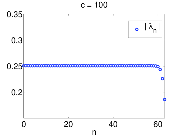
Figure 1: Behavior of $|\lambda_{n}|$ for $0<n<2c/\pi$, with $c=100$. Corresponds to Experiment 1 in Section 5.

The results of Experiment 1 are shown in Table 1 and Figure 1. Table 1 has the following structure. The first two columns contain the band limit $c$ and the prolate index $n$, respectively. The third column contains the ratio of $n$ to $2c/\pi$. The fourth column contains $|\lambda_{n}|$. The last column contains the eigenvalue $\mu_{n}$ of the integral operator $Q_{c}$ (see (6), (10) in Section 2.1).

In Figure 1, we plot $|\lambda_{n}|$, corresponding to $c=100$, as a function of $n$, for integer $n$ between $0$ and $2c/\pi$.

Several observations can be made from Table 1 and Figure 1.

• For all five values of band limit $c$, the eigenvalue $\mu_{n}$ decreases from $\approx 1$ to $\approx 1/2$, as $n$ increases from $0$ to $(2c/\pi)$. In other words, the first $2c/\pi$ eigenvalues $\lambda_{n}$ have roughly the same magnitude $\approx\sqrt{2\pi/c}$. This observation confirms Theorem 2 in Section 2.1.

• Due to Theorem 6 in Section 2.1, the bounds on the decay of $|\lambda_{n}|$, established in Section 4, hold for $n$ greater than $2c/\pi$ only (see also Remark 5). Thus, Table 1 indicates that this assumption on $n$ is, in fact, not restrictive, since the first $2c/\pi$ eigenvalues have roughly constant magnitude.

5.2 Experiment 2

In this experiment, we illustrate Theorem 23. As opposed to Experiment 1, we demonstrate the behavior of $|\lambda_{n}|$ for $n>2c/\pi$.

In this experiment, we proceed as follows. First, we pick band limit $c>0$ (more or less arbitrarily). Then, for each even integer $n$ in the range

$$\frac{2c}{\pi}<n<\frac{2c}{\pi}+20\cdot\log(c),$$ (246)

we evaluate numerically $|\lambda_{n}|$ and $\zeta(n,c)$, where the latter is defined via (182) in Theorem 23.

The results of Experiment 2 are shown in Figures 2 - 4 and in Table 2. In Figures 2 - 4, we plot both $\log(|\lambda_{n}|)$ and $\log(\zeta(n,c))$ as functions of $n$. Each of Figures 2 - 4 corresponds to a certain value of band limit ($c=10,10^{2},10^{3},10^{4},10^{5}$, respectively).

$\varepsilon$	$c$	$n_{1}(\varepsilon)$	$\Delta_{1}(\varepsilon)$	$n_{2}(\varepsilon)$	$\Delta_{2}(\varepsilon)$	$n_{2}(\varepsilon)-n_{1}(\varepsilon)$
$e^{-50}$	10	32	0.11133E+02	38	0.13738E+02	6
$e^{-50}$	$10^{2}$	107	0.94107E+01	114	0.10931E+02	7
$e^{-50}$	$10^{3}$	700	0.91752E+01	712	0.10912E+02	12
$e^{-50}$	$10^{4}$	6450	0.90987E+01	6468	0.11053E+02	18
$e^{-50}$	$10^{5}$	63765	0.89484E+01	63792	0.11294E+02	27
$e^{-100}$	10	50	0.18950E+02	56	0.21556E+02	6
$e^{-100}$	$10^{2}$	138	0.16142E+02	146	0.17879E+02	8
$e^{-100}$	$10^{3}$	753	0.16848E+02	764	0.18440E+02	11
$e^{-100}$	$10^{4}$	6526	0.17350E+02	6542	0.19087E+02	16
$e^{-100}$	$10^{5}$	63864	0.17547E+02	63890	0.19806E+02	26

Table 2: Illustration of Theorem 23. Corresponds to Experiment 2 in Section 5.

Table 2 has the following structure. The first column contains precision $\varepsilon=e^{-50},e^{-100}$. The second column contains band limit $c$. The third column contains the integer $n_{1}(\varepsilon)$, defined via the formula

$$n_{1}(\varepsilon)=\min_{k}\left\{k>2c/\pi\;:\;|\lambda_{k}|<\varepsilon\right\}.$$ (247)

In other words, $n_{1}(\varepsilon)$ is the integer satisfying the inequality

$$|\lambda_{n_{1}(\varepsilon)-1}|>\varepsilon>|\lambda_{n_{1}(\varepsilon)}|.$$ (248)

The fourth column contains $\Delta_{1}(\varepsilon)$, defined to be the difference between $n_{1}(\varepsilon)$ and $2c/\pi$, scaled by $\log(c)$. In other words,

$$\Delta_{1}(\varepsilon)=\frac{n_{1}(\varepsilon)-2c/\pi}{\log(c)}.$$ (249)

The fifth column contains the even integer $n_{2}(\varepsilon)$, defined via the formula

$$n_{2}(\varepsilon)=\min_{k}\left\{k>2c/\pi\;:\;k\text{ is even},\;|\zeta(k,c)|<\varepsilon\right\}.$$ (250)

In other words, $n_{2}(\varepsilon)$ is the even integer satisfying the inequality

$$|\zeta(n_{2}(\varepsilon)-2,c)|>\varepsilon>|\zeta(n_{2}(\varepsilon),c)|.$$ (251)

The sixth column contains $\Delta_{2}(\varepsilon)$, defined to be the difference between $n_{2}(\varepsilon)$ and $2c/\pi$, scaled by $\log(c)$. In other words,

$$\Delta_{2}(\varepsilon)=\frac{n_{2}(\varepsilon)-2c/\pi}{\log(c)}.$$ (252)

The last column contains the difference between $n_{2}(\varepsilon)$ and $n_{1}(\varepsilon)$.

Several observations can be made from Figures 2 - 4 and Table 2.

• In all figures, $|\lambda_{n}|<\zeta(n,c)$, as expected, which confirms Theorem 23.

• For each $c$, both $|\lambda_{n}|$ and $\zeta(n,c)$ decay roughly exponentially fast with $n$.

• For each $c$, both $|\lambda_{n}|$ and $\zeta(n,c)$ decrease to roughly $e^{-125}$, as $n$ increases from $2c/\pi$ to $2c/\pi+20\cdot\log(c)$. In particular,

  $$\left|\lambda_{2c/\pi+20\cdot\log(c)}\right|\approx e^{-125},$$ (253)

  for $c=10,10^{2},10^{3},10^{4},10^{5}$. The fact that the right-hand side of (253) is the same for all $c$ is somewhat surprising. However, this is not coincidental, as will be illustrated in Experiment 3 below.

• For $c=10^{2},10^{3},10^{4},10^{5}$, it suffices to take $n\approx 2c/\pi+9\cdot\log(c)$ to ensure that $|\lambda_{n}|\approx e^{-50}$ (see third column in Table 2). In addition, it suffices to take $n\approx 2c/\pi+17\cdot\log(c)$ to ensure that $|\lambda_{n}|\approx e^{-100}$. In other words,

  $$n_{1}(\varepsilon)\approx\frac{2c}{\pi}+0.17\cdot\log\left(\frac{1}{\varepsilon}\right)\cdot\log(c),$$ (254)

  where $n_{1}(\varepsilon)$ is defined via (247) above (see also (253)).

• For $c=10^{2},10^{3},10^{4},10^{5}$, it suffices to take $n\approx 2c/\pi+11\cdot\log(c)$ to ensure that $\zeta(n,c)\approx e^{-50}$ (see fifth column in Table 2). In addition, it suffices to take $n\approx 2c/\pi+19\cdot\log(c)$ to ensure that $\zeta(n,c)\approx e^{-100}$. In other words,

  $$n_{2}(\varepsilon)\approx\frac{2c}{\pi}+0.2\cdot\log\left(\frac{1}{\varepsilon}\right)\cdot\log(c),$$ (255)

  where $n_{2}(\varepsilon)$ is defined via (250) above (see also (253), (254)).

• The difference $n_{2}(\varepsilon)-n_{1}(\varepsilon)$ is roughly independent of $\varepsilon$, and grows only slowly as $c$ increases (see last column of Table 2). In other words, suppose that one needs to determine $n$ such that $|\lambda_{k}|<e^{-50}$ for all $k\geq n$. Due to (247), $n_{1}(e^{-50})$ would be the minimal such $n$. On the other hand, $n=n_{2}(e^{-50})$ is only larger by 6 for $c=10$ and by 27 for $c=10^{5}$.

5.3 Experiment 3

In this experiment, we illustrate Theorem 32. We proceed as follows. First, we pick band limit $c>0$ (more or less arbitrarily). Then, we define the positive integer $n_{\max}$ to be the minimal even integer such that

$$n_{\max}>\frac{2c}{\pi}+\frac{2}{\pi^{2}}\cdot 150\cdot\log\left(\frac{4e\pi c}{150}\right)\approx\frac{2c}{\pi}+30.4\cdot\log(0.23\cdot c).$$ (256)

Then, for each positive even integer $n$ in the range

$$\frac{2c}{\pi}<n<n_{\max},$$ (257)

we evaluate the following quantities:

• the eigenvalue $\lambda_{n}$ of the operator $F_{c}$ (see (4), (5) in Section 2.1);

• $\delta(n)$ of Definition 1 in Section 4.3;

• $\zeta(n,c)$, defined via (182) in Theorem 23 in Section 4.2;

• $\xi(n,c)$, defined via (226) in Theorem 32 in Section 4.3.

The results of Experiment 3 are shown in Figures 5(a), 5(b), that correspond, respectively, to band limit $c=10^{4}$ and $c=10^{5}$. In each of Figures 5(a), 5(b), we plot $\log(|\lambda_{n}|)$, $-\delta(n)$, $\log(\zeta(n,c))$ and $\log(\xi(n,c))$ as functions of $n$.

Several observations can be made from Figures 5(a), 5(b), and from more detailed experiments by the author.

• In both figures,

  $$\log(|\lambda_{n}|)<-\delta(n)<\log(\zeta(n,c))<\log(\xi(n,c)),$$ (258)

  for all $n$. This observation confirms both Theorem 23 of Section 4.2 and Theorem 32 of Section 4.3. Also, $\xi(n,c)$ is weaker than $\zeta(n,c)$ as an upper bound on $|\lambda_{n}|$, as expected.

• All the four functions, plotted in Figures 5(a), 5(b), decay roughly exponentially with $n$. Moreover,

  $$\log(|\lambda_{n}|)\approx\log\sqrt{\frac{2\pi}{c}}-\delta(n),$$ (259)

  in correspondence with Theorem 5 in Section 2.1. In particular, even the weakest bound $\xi(n,c)$ correctly captures the exponential decay of $|\lambda_{n}|$. On the other hand, $\xi(n,c)$ overestimates $|\lambda_{n}|$ by a roughly constant factor of order $c^{3/2}$ (see also Section 3.2).

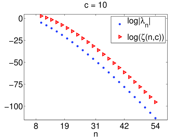
Figure 2: Illustration of Theorem 23 with $c=10$. Corresponds to Experiment 2 in Section 5.

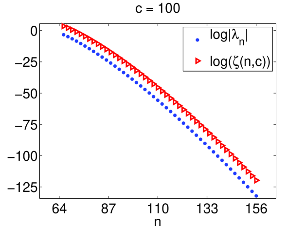
(a) $c=100$.

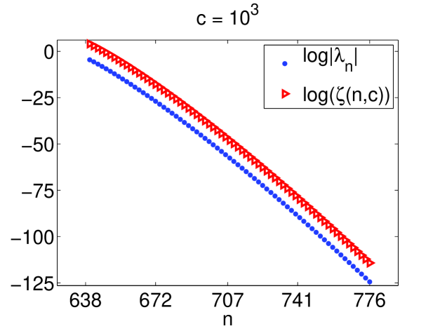
(b) $c=1,000$.

Figure 3: Illustration of Theorem 23. Corresponds to Experiment 2 in Section 5.

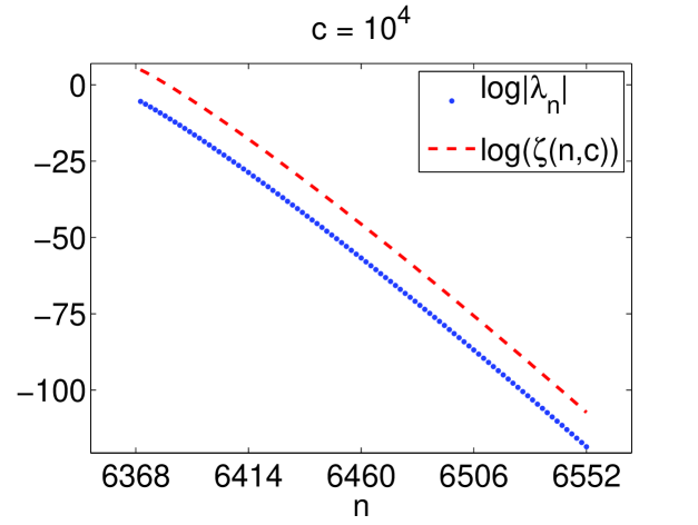
(a) $c=10,000$.

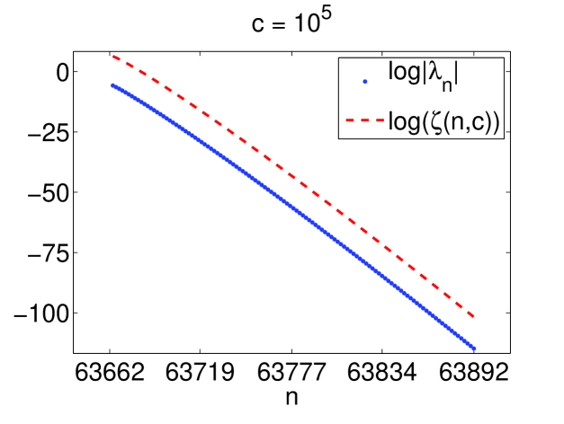
(b) $c=100,000$.

Figure 4: Illustration of Theorem 23. Corresponds to Experiment 2 in Section 5.

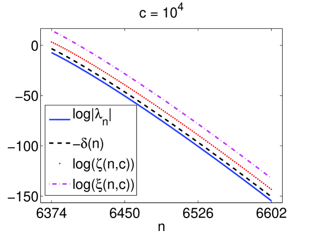
(a) $c=10,000$.

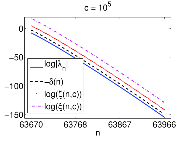
(b) $c=100,000$.

Figure 5: Illustration of Theorem 32. Corresponds to Experiment 3 in Section 5.

References

- [1] Yoel Shkolnisky, Mark Tygert, Vladimir Rokhlin, Approximation of Bandlimited Functions, Appl. Comput. Harmon. Anal. 21, No. 3, 413-420 (2006).
- [2] Andreas Glaser, Xiangtao Liu, Vladimir Rokhlin, A fast algorithm for the calculation of the roots of special functions, SIAM J. Sci. Comput. 29, No. 4, 1420-1438 (2007).
- [3] H. Xiao, V. Rokhlin, N. Yarvin, Prolate spheroidal wavefunctions, quadrature and interpolation, Inverse Probl. 17, No.4, 805-838 (2001).
- [4] Vladimir Rokhlin, Hong Xiao, Approximate Formulae for Certain Prolate Spheroidal Wave Functions Valid for Large Value of Both Order and Band Limit, Appl. Comput. Harmon. Anal. 22, No. 1, 105-123 (2007).
- [5] Hong Xiao, Vladimir Rokhlin, High-frequency asymptotic expansions for certain prolate spheroidal wave functions, J. Fourier Anal. Appl. 9, No. 6, 575-596 (2003).
- [6] H. J. Landau, H. Widom, Eigenvalue distribution of time and frequency limiting, J. Math. Anal. Appl. 77, 469-481 (1980).
- [7] I.S. Gradshteyn, I.M. Ryzhik, Table of Integrals, Series, and Products, Seventh Edition, Elsevier Inc., 2007.
- [8] D. Slepian, H. O. Pollak, Prolate spheroidal wave functions, Fourier analysis, and uncertainty - I, Bell System Tech. J. 40, 43-63 (1961).
- [9] H. J. Landau, H. O. Pollak, Prolate spheroidal wave functions, Fourier analysis, and uncertainty - II, Bell System Tech. J. 40, 65-84 (1961).
- [10] H. J. Landau, H. O. Pollak, Prolate spheroidal wave functions, Fourier analysis, and uncertainty - III: the dimension of space of essentially time- and band-limited signals, Bell System Tech. J. 41, 1295-1336 (1962).
- [11] D. Slepian, H. O. Pollak, Prolate spheroidal wave functions, Fourier analysis, and uncertainty - IV: extensions to many dimensions, generalized prolate spheroidal wave functions, Bell Syst. Tech. J. November 3009-57 (1964).
- [12] D. Slepian, Prolate spheroidal wave functions, Fourier analysis, and uncertainty - V: the discrete case, Bell. System Techn. J. 57, 1371-1430 (1978).
- [13] D. Slepian, Some comments on Fourier analysis, uncertainty, and modeling, SIAM Rev. 25, 379-393 (1983).
- [14] D. Slepian, Some asymptotic expansions for prolate spheroidal wave functions, J. Math. Phys. 44 99-140 (1965).
- [15] D. Slepian, E. Sonnenblick, Eigenvalues associated with prolate spheroidal wave functions of zero order, Bell Syst. Tech. J. 1745-1759, 1965.
- [16] P. M. Morse, H. Feshbach, Methods of Theoretical Physics, New York McGraw-Hill, 1953.
- [17] W. H. J. Fuchs, On the eigenvalues of an integral equation arising in the theory of band-limited signals, J. Math. Anal. Appl. 9 317-330 (1964).
- [18] F. A. Grünbaum, L. Longhi, M. Perlstadt, Differential operators commuting with finite convolution integral operators: some non-Abelian examples, SIAM J. Appl. Math. 42, 941-955 (1982).
- [19] C. Flammer, Spheroidal Wave Functions, Stanford, CA: Stanford University Press, 1956.
- [20] A. Papoulis, Signal Analysis, Mc-Graw Hill, Inc., 1977.
- [21] M. Abramowitz, I. A. Stegun, Handbook of Mathematical Functions with Formulas, Graphs and Mathematical Tables, Dover Publications, 1964.
- [22] A. Osipov, Non-asymptotic Analysis of Bandlimited Functions, Yale CS Technical Report #1449, 2012.
- [23] A. Osipov, Certain inequalities involving prolate spheroidal wave functions and associated quantities, arXiv:1206.4056v1, 2012.