The Cosmic Infrared Background Experiment (CIBER): The Wide-Field Imagers

Abstract

We have developed and characterized an imaging instrument to measure the spatial properties of the diffuse near-infrared extragalactic background light in a search for fluctuations from $z>6$ galaxies during the epoch of reionization. The instrument is part of the Cosmic Infrared Background Experiment (CIBER), designed to observe the extragalactic background light above the Earth’s atmosphere during a suborbital sounding rocket flight. The imaging instrument incorporates a $2^{\circ}\times 2^{\circ}$ field of view, to measure fluctuations over the predicted peak of the spatial power spectrum at 10 arcminutes, and $7^{\prime\prime}\times 7^{\prime\prime}$ pixels, to remove lower redshift galaxies to a depth sufficient to reduce the low-redshift galaxy clustering foreground below instrumental sensitivity. The imaging instrument employs two cameras with $\Delta\lambda/\lambda\sim 0.5$ bandpasses centered at $1.1\,\mu$m and $1.6\,\mu$m to spectrally discriminate reionization extragalactic background fluctuations from local foreground fluctuations. CIBER operates at wavelengths where the electromagnetic spectrum of the reionization extragalactic background is thought to peak, and complements fluctuations measurements by AKARI and Spitzer at longer wavelengths. We have characterized the instrument in the laboratory, including measurements of the sensitivity, flat-field response, stray light performance, and noise properties. Several modifications were made to the instrument following a first flight in 2009 February. The instrument performed to specifications in subsequent flights in 2010 July and 2012 March, and the scientific data are now being analyzed.

1. Introduction

The extragalactic background light (EBL) is a measure of the integrated radiation produced by stellar nucleosynthesis and gravitational accretion over cosmic history. The EBL must contain the radiation produced during the epoch of reionization (the reionization-EBL, or simply the REBL). The REBL comes from the UV and optical photons emitted by the first ionizing stars and stellar remnants, radiation that is now redshifted into the near-infrared (NIR). The REBL is expected to peak at 1-2 um due to the redshifted Lyman-$\alpha$ and Lyman-break features. Furthermore while the brightness of the REBL must be sufficient to initiate and sustain ionization, the individual sources may be quite faint (Salvaterra et al., 2011).

We have developed a specialized imaging instrument to measure REBL spatial fluctuations, consisting of two wide-field cameras that are part of the Cosmic Infrared Background Experiment (CIBER; Bock et al. 2006), developed to measure the absolute intensity, spectrum, and spatial properties of the EBL. CIBER’s imaging cameras are combined with a low-resolution spectrometer (LRS; Tsumura et al. 2012) designed to measure the absolute sky brightness at wavelengths $0.75<\lambda<2.1\,\mu$m, and a narrow-band spectrometer (NBS; Korngut et al. 2012) designed to measure the absolute ZL intensity using the $854.2\,$nm Ca II Fraunhofer line. A full description of the CIBER payload, including the overall mechanical and thermal design, and detailed descriptions of the focal plane housings, calibration lamps, shutters, electronic systems, telemetry and data handling, laboratory calibration equipment, flight events, and flight thermal performance, is given in Zemcov et al. (2012). The observation sequence and science targets from the first flight are available in Tsumura et al. (2010).

In this paper, we describe the scientific background of EBL fluctuation measurements in sections 1.1 and 1.2, the instrument design in section 2, laboratory instrument characterization in section 3, modifications following the first flight in section 4, and performance in the second flight in section 5. Sensitivity calculations are given in a short appendix.

1.1. Science Background

Searching for the REBL appears to be more tractable in a multi-color fluctuations measurement than by absolute photometry. Absolute photometry, measuring the sky brightness with a photometer and removing local foregrounds, has proven to be problematic in the NIR, where the main difficulty is subtracting the Zodiacal light (ZL) foreground, which is a combination of scattered sunlight and thermal emission from interplanetary dust grains in our solar system. However, absolute photometry studies give consistent results in the far-infrared (Hauser et al. 1998, Fixsen et al. 1998, Juvela et al. 2009, Matsuura et al. 2011, Pénin et al. 2011). These far-infrared measurements are close to the EBL derived from galaxy counts though statistical and lensing techniques that probe below the confusion limit (Marsden et al. 2009, Zemcov et al. 2010, Béthermin et al. 2010, Berta et al. 2010). However in the NIR, at wavelengths appropriate for a REBL search, absolute EBL measurements are not internally consistent (Cambrésy et al. 2001, Dwek & Arendt 1998, Matsumoto et al. 2005, Wright 2001, Levenson & Wright 2008). A significant component of this disagreement is related to the choice of model used to subtract ZL (Kelsall et al. 1998, Wright 2001). Furthermore, some absolute EBL measurements (Cambrésy et al. 2001, Matsumoto et al. 2005) are significantly higher than the integrated galaxy light derived from source counts (Madau & Pozzetti 2000, Totani et al. 2001, Levenson et al. 2007, Keenan et al. 2010).

The current disagreement between absolute measurements and galaxy counts are difficult to reconcile with theoretical calculations (Madau & Silk, 2005) or TeV absorption measurements from blazars (Gilmore 2001, Aharonian et al. 2006, Schroedter 2005). However TeV constraints on the NIR EBL require an assumption about the intrinsic blazar spectrum (Dwek et al., 2005). Furthermore cosmic rays produced at the blazar are not attenuated by the EBL and can produce secondary gamma rays that may explain the current TeV data without placing a serious constraint on the NIR EBL (Essey & Kusenko, 2010).

Instead of measuring the absolute sky brightness, it is possible to detect or constrain the REBL by studying the spatial properties of the background (Cooray et al. 2004, Kashlinsky et al. 2004). A spatial power spectrum of the EBL contains a REBL clustering component, evident at an angular scale of approximately 10 arcminutes as shown in Figure 1, that is related to the underlying power spectrum of dark matter. Numerical simulations of first galaxy formation indicate the effects of non-linear clustering are significant (Fernandez et al., 2010). There are also REBL fluctuations from the Poisson (unclustered shot noise) component, but the amplitude of this term is more difficult to predict as it is related to the number counts of the first galaxies, that is, the brightness distribution and surface density of sources. In addition, REBL fluctuations are thought to have a characteristic electromagnetic spectrum, peaking at the redshift-integrated Lyman-$\alpha$ emission feature. If reionization occurs at $z\sim 10$, this emission peak is redshifted into the NIR, with a spectral shape that depends on the luminosity and duration of the epoch of reionization.

Early measurements with the Diffuse Infrared Background Experiment (DIRBE; Kashlinsky & Odenwald 2000) and the Infrared Telescope in Space (IRTS; Matsumoto et al. 2005) used fluctuations as a tracer of the total EBL. A first detection of REBL fluctuations was reported by Kashlinsky et al. (2005) using the Spitzer Infrared Array Camera (IRAC; Fazio et al. 2004) in the 3.6 and $4.5\,\mu$m bands in $5\times 5$ arcminute regions, corresponding to the IRAC field of view. The authors observe a departure from Poisson noise on $1{-}5$ arcminute scales which they attribute to first-light galaxies, after ruling out Zodiacal, Galactic, and galaxy clustering foregrounds. The observed brightness of the fluctuations is approximately constant at 3.6 and $4.5\,\mu$m. This analysis was later extended to $10\times 10\,$arcmin fields, giving similar results (Kashlinsky et al., 2007). Thompson et al. (2007a) studied a $144\times 144\,$arcsec field with the Hubble Space Telescope (HST) at 1.1 and $1.6\,\mu$m, finding no evidence for $z>8$ galaxies contributing to the HST or the Spitzer fluctuations (Thompson et al., 2007b). Finally, Matsumoto et al. (2011) report first-light galaxy fluctuations with AKARI at 2.4, 3.2 and $4.1\,\mu$m in a 10 arcminute field. Their reported spectrum shows a strong increase from 4.1 to $2.4\,\mu$m, consistent with a Rayleigh-Jeans spectrum.

In Figure 1 we show two predictions related to the angular power spectrum of REBL anisotropies. The lower prediction (solid red line) is from Cooray et al. (2012), derived from the observed luminosity functions of Lyman dropout galaxies at redshifts of 6, 7 and 8 (Bouwens et al., 2008) at the bright end. The reionization history involves an optical depth to electron scattering of 0.09, consistent with the WMAP 7-year measurement of $\tau=0.088\pm 0.014$ (Komatsu et al., 2011). The absolute REBL background is $0.3\,nWm^{-2}sr^{-1}$ at 3.6 $\mu$m for this model. Cooray et al. (2012) improved on previous predictions (Cooray et al., 2004) by accounting for non-linear clustering at small angular scales with a halo model for reionization galaxies at $z>6$. Note that the REBL fluctuation power is similar at 1.6 and 1.1 $\mu$m given the redshift of reionization is around at $z\sim 10$.

The upper prediction (dashed red line) is normalized to the anisotropy amplitude level reported by Spitzer-IRAC at 3.6 $\mu$m (Kashlinsky et al., 2005). This power spectrum requires an absolute REBL background between 2 to 3 $nWm^{-2}sr^{-1}$ at 3.6 $\mu$m. We scale the power spectra to shorter wavelengths based on a Rayleigh-Jeans spectrum, consistent with the combined measurements of Spitzer and AKARI (Matsumoto et al., 2011).

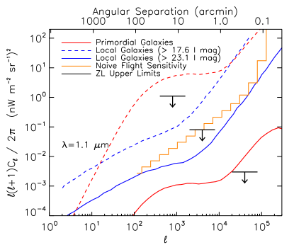
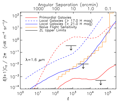
Figure 1.— Power spectra of REBL and foreground fluctuations at $1.1\,\mu$m (left) and $1.6\,\mu$m (right). In both cases the clustering power spectra of local ($z<3$) galaxies, for sources brighter than two different magnitude cutoffs, are shown as the blue solid and dashed lines. These galaxy clustering power spectra are based on measured fluctuations as a function of cutoff magnitude from Sullivan et al. (2007) and are consistent with the predictions by Helgason et al. (2012) based on a large compilation of galaxy luminosity functions between $z=0$ and 4. The two red lines correspond to two expectations on the REBL anisotropy power spectrum as described in section 1.1. Upper limits to the ZL fluctuation power, shown in black, are scaled from experimental upper limits at longer wavelengths by the ZL spectrum. The predicted CIBER sensitivities in both bands are shown in orange. These are calculated with the instrument parameters listed in Table 2 assuming that the detector noise given in Table 4 is uncorrelated and Gaussian over the array and using the $\Delta C_{\ell}$ formalism in Knox (1995).

Fluctuation measurements are only feasible if the contributions from foregrounds can be removed. Fortunately, it appears easier to remove foregrounds in fluctuation measurements than in absolute photometry measurements. The largest foreground, ZL, is known to be spatially uniform on spatial scales smaller than a degree (Abraham et al. 1997, Kashlinsky et al. 2005, Pyo & et al. 2011). Furthermore, any spatial variations in ZL can be monitored and removed by observing a field over a period of time, as the view through the interplanetary dust cloud changes annually. Galaxies and stars give spatial fluctuations from Poisson variations and clustering. These can be eliminated by masking sources from the image, either through detection or by using an external catalog of known sources. Galaxy clustering, arguably the most serious of these potential contaminants, requires a sufficiently deep source cutoff to reduce the clustering spectrum below the level of REBL fluctuations by masking sources.

1.2. Theoretical Design Drivers

These early fluctuation results call for a next generation of improved measurements at shorter wavelengths, spanning the expected peak of the REBL electromagnetic spectrum, with wide angular coverage, to definitively measure the expected peak in the REBL spatial power spectrum. In order to make a definitive REBL fluctuations measurement, we require: (1) a wide field of view to allow measurements of the characteristic REBL spatial power spectrum, (2) observations in multiple NIR bands in order to characterize the REBL electromagnetic spectrum and distinguish it from potential foregrounds, and (3) arcsecond angular resolution to remove galaxies to a sufficient depth to minimize the galaxy clustering foreground signal.

High-fidelity spatial imaging on degree scales is problematic in the NIR due to airglow emission from the Earth’s atmosphere, which is some $200{-}1500$ times brighter than the astrophysical sky in the NIR J, H and K bands (Allen, 1976). Airglow emission has time-variable structure (Ramsay et al., 1992) with spatial variations that increase on larger angular scales, especially from $1^{\circ}$ to $10^{\circ}$ (Adams & Skrutskie, 1996). We therefore conduct observations on a sounding rocket flight, at altitudes above the layers in the atmosphere responsible for airglow emission at characteristic altitudes of $\sim 100\,$km. To measure the $\sim 10^{\prime}$ peak in the REBL spatial power spectrum, it is necessary to image an area of sky on the order of a square degree. While one can image a large field with a mosaic using a small field of view, this requires a highly stable instrument. A wide field of view allows a measurement using single exposures in the short time available on a sounding rocket flight.

The REBL electromagnetic spectrum is predicted to peak at $1{-}2\,\mu$m (Cooray et al. 2004, Kashlinsky et al. 2004) due to the redshift-integrated Lyman-$\alpha$ emission feature, with a decreasing spectrum at longer wavelengths that depends on the history of reionization and the presence of free-free emission from ionized gas surrounding the first galaxies. Observations in the optical and near-IR should detect this spectrum, which is distinct from that of local foregrounds, namely ZL, stars, galaxies, scattered starlight (i.e. diffuse galactic light), and other Galactic emission. Though ideally the wavelength coverage would extend out to $\sim 5\,\mu$m, the key wavelengths for REBL science bracket the $1{-}2\,\mu$m peak. Longer wavelength information can be obtained by cross-correlating CIBER data with overlapping wide-field Spitzer and AKARI maps.

The local-galaxy fluctuations foreground is mitigated by masking galaxies down to a given flux threshold. The masking depth needed depends on the residual clustering and Poisson fluctuations of galaxies below the cutoff flux. Sullivan et al. (2007) measured galaxy clustering as a function of cutoff from a wide-field ground-based NIR survey catalog. We note that the REBL is best discriminated from low-redshift galaxy clustering and Poisson fluctuations at  10 arcminutes, as is evident in Figure 1 by comparing the REBL and galaxy clustering power spectra. Thus wide-field observations are also helpful for discriminating REBL from local galaxy fluctuations.

The flux cutoff needed to separate the optimistic REBL model from local galaxy fluctuations is $\sim 17^{th}$ Vega magnitude at $1.6\,\mu$m, as is evident from the curves in Figure 1. The spatial density of galaxies brighter than $17^{th}$ Vega magnitude is $N(>S)=500$ galaxies per square degree. The cutoff required to remove galaxies well below the expected CIBER instrument sensitivity is $\sim 23^{rd}$ Vega magnitude at $1.6\,\mu$m, corresponding to $N(>S)=1.5\times 10^{5}$ galaxies per square degree. Thus we find an angular resolution of $4{-}80$ arcseconds is needed to remove galaxies in order to lose less than 25 % of the pixels from masking.

Galaxy masking can be accomplished using ancillary observations with greater point source depth, masking pixels in the CIBER images below the CIBER point source sensitivity. The fields observed in the first two flights of CIBER, listed in Table 1, allows source masking using deep companion catalogs obtained in ground based NIR observations. Details on first flight observations of these fields is available in Tsumura et al. (2010). These fields have also been observed in a search for REBL fluctuations by AKARI and Spitzer at longer wavelengths, allowing for a cross-correlation analysis with CIBER.

Table 1CIBER Survey Fields and Ancillary Data Depths.

CIBER Field	Ancillary	$\lambda$	Field Coverage	Ancillary Depth		Reference
	Coverage	($\mu$m)	(%)	(Vega mag)	($\sigma$)
Boötes	NDWFS	0.83	100	25.5	5	Jannuzi & Dey (1999)
	NEWFIRM	1.0	100	22.0	5	Gonzalez et al. (2011)
	NEWFIRM	1.6	100	20.8	5	Gonzalez et al. (2011)
	NEWFIRM	2.4	100	19.5	5	Gonzalez et al. (2011)
	Spitzer-SDWFS	3.6	100	19.7	5	Ashby et al. (2009)
North Ecliptic Pole	Maidanak	0.9	60	21.9	5	Jeon et al. (2010)
	CFHT	1.2	50	24	4	Hwang et al. (2007)
	2MASS	1.6	100	17.9	10	Cutri et al. (2003)
	AKARI	2.4	98	19.7	5	Lee et al. (2009)
ELIAS-N1	UKIDSS-DR6	0.9	75	22.3	5	Lawrence et al. (2007)
	INT	0.9	100	21.9	5	González-Solares et al. (2011)
	2MASS	1.6	100	17.8	10	Cutri et al. (2003)
	Spitzer-SWIRE	3.6	100	18.6	10	Lonsdale et al. (2003)

2. Instrument Design

The Imager instrument consists of two wide-field refracting NIR telescopes each with an $11\,$cm aperture, combined with band-defining filters, a cold shutter, and a $1024\times 1024$ HgCdTe $2.5\,\mu$m Hawaii-1 focal plane array. The Imager optics were designed and built by Genesia Corporation using the cryogenic index of refraction measurements of Yamamuro et al. (2006). A schematic of the assembly is shown in Figure 2. The assembly housing the Imager optics are constructed from aluminum alloy 6061, and the lenses are made from anti-reflection coated Silica, S-FPL53 and S-TIL25 glass. The assembly is carefully designed to maintain optical alignment and focus through launch acceleration and vibration. The aluminum housing is hard black anodized to reduce reflections inside the cryogenic insert and telescope assembly, with the exception of the static baffle at the front of the assembly which is gold plated on its external surface and Epner laser black coated on its inner surface. This scheme serves to reduce the absorptivity of the baffle on the side facing warm components at the front of the payload section, and increase the absorptivity to NIR light on the inside. At the other end of the camera, a focal plane assembly is mounted to the back of the optical assembly and thermally isolated using Vespel SP-1 standoffs. The assembly includes a cold shutter and active thermal control for each detector. In addition, a calibration lamp system illuminates the focal plane in a repeatable way to provide a transfer standard during flight. The design of the calibration lamp system is common to all of the CIBER instruments and is presented in Zemcov et al. (2012).

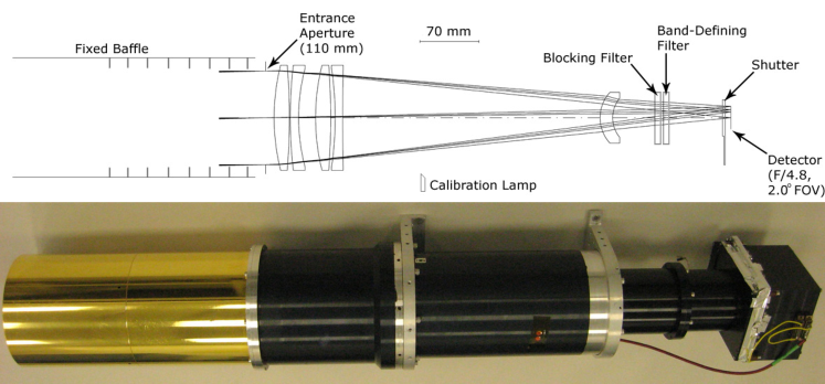
Figure 2.— Schematic and photograph of the CIBER imaging camera. Light enters the optical system at left and is imaged to the focal plane at right. A fixed baffle is used to reduce scattering on the first optic. The Imager assembly employs a fiber-fed calibration lamp system, band-defining and blocking filters, and a focal plane assembly as described in Zemcov et al. (2012). Both Imager assemblies used in CIBER are identical except for their band defining filters, set with $\Delta\lambda/\lambda\sim 0.5$ bandpasses centered at $1.1\,\mu$m and $1.6\,\mu$m, roughly corresponding to astronomical I and H band. The photograph shows a fully assembled Imager in the lab. The entire assembly mounts to the CIBER optical bench when installed in the payload and operates at $\sim 80\,$K.

The optical transmittance of the two Imager filters are shown in Figure 3. The filter stack is located behind the optical elements and in front of the focal plane assembly and cold shutter as shown in Figure 2. Each lens provides additional filtering for wavelengths that are out of band for both instruments, as their anti-reflection coatings transmit less than 1.5% of light with wavelengths shorter than $0.75\,\mu$m or longer than $2.0\,\mu$m.

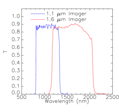
Figure 3.— $1.1\,\mu$m and $1.6\,\mu$m Imager filter responses. These curves represent the transmission of the optical stack which includes band defining and blocking filters as well as 5 anti-reflection coated lenses. This response does not include the response of the detector array, which typically cuts off at $\sim 900\,$nm for a Hawaii-1 array with a sapphire substrate (Mark Farris, private communication).

Table 2 summarizes the design properties of the optics and detector system, and the measured efficiencies, bands, and read noise for the two cameras. The optical efficiency is the product of the reflectance and absorption of the anti-reflection coated lenses taken from witness samples. The instrument performance is calculated in the appendix based on data from Table 2 and presented in Table 4.

Table 2Imager Instrument Properties.

	1.1 $\mu$m Band	1.6 $\mu$m Band	Units
Wavelength Range	$900{-}1320\ast$	$1150{-}2040$	nm
Pupil Diameter	110	110	mm
F#	4.95	4.95
Focal Length	545	545	mm
Pixel Size	$7\times 7$	$7\times 7$	arcsec
Field of View	$2.0\times 2.0$	$2.0\times 2.0$	deg
Optics Efficiency	0.90	0.90
Filter Efficiency	0.92	0.89
Array QE	0.51	0.70	$\ast\ast$
Total Efficiency	0.42	0.56
Array Format	$1024^{2}$	$1024^{2}$
Pixel Pitch	18	18	$\mu$m
Read Noise (CDS)	10	9	e-
Frame Interval	1.78	1.78	s
$\ast$ We assume a $900\,$nm cut-on wavelength from the
Hawaii-1 substrate.
$\ast\ast$ Array QE is estimated from QE measured at $2.2\,\mu$m
for each array and scaled based on the response of
a typical Hawaii-1.

Once assembled, the cameras mount to an optical bench shared with the LRS and NBS. The completed instrument section is then inserted into the experiment vacuum skin. Like the other CIBER instruments, the Imager optics are cooled to $\sim 80\,$K to reduce their in-band emission using a liquid nitrogen cryostat system. Zemcov et al. (2012) describes the various payload configurations used in calibration and in flight which allow both dark and optical testing in the laboratory.

3. Instrument Characterization

REBL fluctuation measurements place demanding requirements on the instrument, including the detector noise properties, linearity and transient response, optical focus, control of stray radiation, and knowledge of the flat field response. We have carried out a series of laboratory measurements to characterize these properties.

3.1. Dark Current

The detector dark current is measured in both flight and laboratory configurations by closing the cold shutters, which attenuate the optical signal by a measured factor of $\sim 10^{3}$. Array data are acquired at $6.8\,\mu$s per pixel sample, so that the full array is read in $1.78\,$s. The pixels are read non-destructively, and integrate charge until reset. The integration time may be selected, but the flight integrations are typically $\sim 50\,$s. To maximize the signal-to-noise ratio, for each pixel we fit the measured output voltage to a slope and an offset as described in Garnett & Forrest (1993). All CIBER Imager data are analyzed using this method, except where noted.

The measured dark current also depends on the detector thermal stability. For the Imagers we require dark current stability of $0.1\,$e${}^{-}/$s, which is equivalent to $\pm 100\,\mu$K/s given a temperature coefficient of $1000\,$e^-/K. The Imager detector arrays are controlled to $\pm 10\,\mu$K/s both in the lab and in flight, exceeding this specification (Zemcov et al., 2012). In the flight configuration with the cold shutter closed and the focal plane under active thermal control, we achieve $\sim 0.3\,$e${}^{-}/$s mean dark current, as shown in Figure 4. The dark current is measured frequently before launch as a monitor of the instrument stability and is entirely consistent with the dark current measured in the laboratory. The stability of the dark current from run to run indicates the dominant contributor to dark current is the array itself, as opposed to temperature or bias drift.

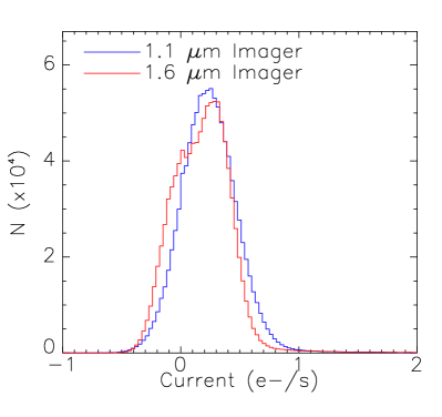
Figure 4.— CIBER Imager dark currents for both cameras. The mean dark current is $0.3\,$e${}^{-}/$s, which is consistent with the manufacturer’s specifications for Hawaii-1 arrays operating near LN₂ temperature.

3.2. Noise Performance

Measuring the REBL spatial power spectrum requires a precise understanding of the noise properties of the array. The array noise introduces a bias that must be accounted and removed in auto-correlation analysis, and determines the uncertainty in the measured power spectrum. The instrument sensitivity shown in Figure 1 assumes the noise over the array is uncorrelated between pixels. Unfortunately, HgCdTe arrays exhibit correlated noise, as described by Moseley et al. (2010). This noise is associated with pickup from the clock drivers to the signal lines, with $1/f$ noise in the multiplexer readout, and depending on the implementation, with $1/f$ noise on the bias and reference voltages supplied to the array.

3.2.1 Noise Model

We characterized array noise using dark laboratory images and data obtained just prior to flight. We first took a series of dark integrations to characterize the noise behavior similar to the $\sim 50\,$s integrations used in flight. In the left hand panels of Figure 5 we show the two dimensional power spectrum of the difference of two consecutive $50\,$s laboratory integrations. The spectrum shows enhanced noise at low spatial frequencies along the read direction that is largely independent of the cross-read spatial frequency, symptomatic of correlated noise in the readout.

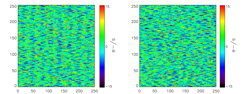
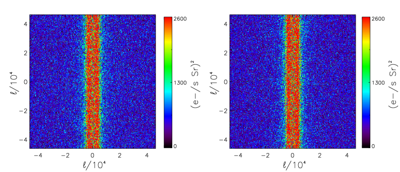
Figure 5.— Images (top) and two dimensional power spectra (bottom) of the difference between two dark images, each obtained in a $50\,$s integration. The upper and lower left hand panels show the image and power spectra of data taken minutes before flight, while the two right hand panels show the same for random realizations using the noise model presented in Section 3.2. The spatial scale of these images has been restricted to $250\times 250$ pixels to better show the spatial structure. In both cases the read direction is horizontal along pixel rows. The vertical structure in the two dimensional power spectra shows increased noise power in the read direction on scales $>50$ pixels. The noise model accurately captures this behavior, both in real and Fourier space.

We then generate an estimate of the noise by constructing time streams for the array readout. First, we determine the best fit slope and offset for each pixel. We then subtract this estimate of the photo current signal in each pixel in each frame. Finally, we form a sequence of data for each of the four readout quadrants in the order that the readout addresses individual pixels. An example of time-ordered data and its noise spectrum is shown in Figure 6, exhibiting excess noise behavior similar to that described in Moseley et al. (2010).

Figure 6.— The upper panel shows $30\,$ms of signal-subtracted time ordered data from the $1.6\,\mu$m Imager. The lower panel shows the noise spectrum derived from a longer such time series of reads over $50\,$s. The noise increases at $\sim 10\,$kHz, visible in the time stream in the upper panel as the characteristic scale of the noise at $\sim 0.5\,$ms. The ringing visible in the power spectrum below $10\,$kHz corresponds to the harmonics of the clock signals used to address the array.

The correlated noise in the readout may reduce the in-flight sensitivity, and must be modeled to remove noise bias in the auto-correlation power spectra. While a full description of a noise model of the flight data is outside the scope of this paper, we can generate a model confined to the noise properties of the arrays observed in laboratory testing. This model is generated by producing a Gaussian noise realization of the power spectrum given in Figure 6. This is used to generate random realizations of time ordered data. These data are mapped back into raw frames, and fit to slopes and offsets to determine the images for a full $50\,$s integration. To generate images like those shown in Figure 5, we generate multiple images and display the difference of two $50\,$s images. This formalism will be extended to the flight data by adding photon shot noise from the astrophysical sky, and correcting for source masking, in a future publication.

3.2.2 Estimated Flight Sensitivity

To calculate the effect of correlated noise on the final science sensitivity, we take our sequence of dark laboratory images, calculate the two dimensional power spectrum, and apply a two-dimensional Fourier mask that removes modes sensitive to the excess low frequency noise. We remove these modes because they have a phase coherence in real data that is not fully captured by the Gaussian noise model. After Fourier masking, we calculate the spatial power in logarithmic multipole bins. We then evaluate the standard deviation in the spatial power among eight dark images, and refer this to sky brightness units using the measured calibration factors in Table 4. Because the laboratory data do not have appreciable photon noise, we add an estimate of uncorrelated photon noise from the flight photo currents. We compare this empirical determination of the noise with the naïve sensitivity calculation in Figure 7 (Knox, 1995). The empirical noise is close to the naïve calculation on small spatial frequencies, but is degraded by correlated noise on large spatial scales. However the instrument is still sufficiently sensitive to easily detect the optimistic REBL power spectrum. For future experiments, one may address the reference pixels in Hawaii-RG arrays to mitigate the effects of correlated noise.

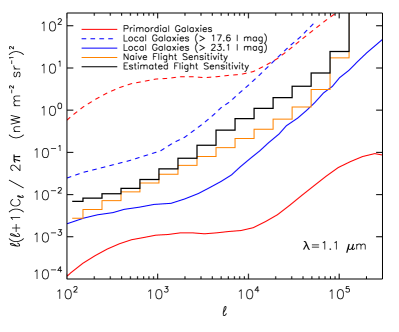
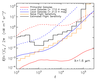
Figure 7.— The Imager sensitivity to REBL fluctuations. The left hand panel shows the estimated sensitivity for the $1.1\,\mu$m channel, and the right for the $1.6\,\mu$m channel. In addition to the curves taken from Figure 1, we show the sensitivity derived from laboratory data for both bands as described in the text using the same $\ell$ binning as the naïve sensitivity estimate shown by the orange curve. The black curve is an estimate of the flight sensitivity, combining measured laboratory noise from an ensemble of $50\,$s integrations, added with uncorrelated photon noise derived from the flight photo currents. This estimate is for a single $50\,$s integration, and does not include the effects of noise in the flat field or the loss of pixels from galaxy masking.

3.3. Detector Non-linearity and Saturation

The Imager detectors have a dynamic range over which the response tracks the source brightness in a linear fashion. As is typical for Hawaii-1 detectors, the full well depth is measured to be $\sim 10^{5}\,$e^-; however, the detectors begin to deviate from linearity well before this. In order to flag detector non-linearity, we find pixels with different illumination levels and track their behavior during an integration. Figure 8 shows the typical response of a pixel to a bright $\sim 3500\,$e${}^{-}/$s source over time. This plot shows a deviation from the linear model which is large at half the full well depth. Except for a few bright stars, Imager flight data are well within the linear regime. Pixels with an integrated charge greater than $7000\,e^{-}$ have a non-linearity $\sim 1\%$ are simply flagged and removed from further analysis, amounting to a pixel loss of $<0.5\%$ over the array.

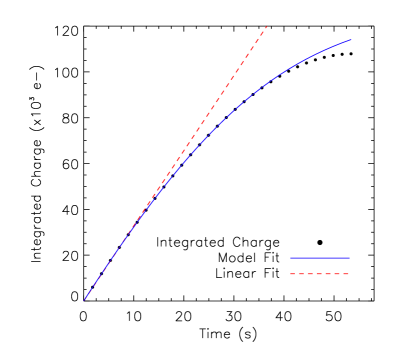
Figure 8.— Integrated signal as a function of time for a typical Imager pixel. The black data show subsequent reads of the Imager detector for an incident brightness of $\sim 3500\,$e${}^{-}/$s. The dashed red line shows the linear model matching the slope of the first $10\,$s of the integration. Finally, the blue line is a fit to the model from Biesiadzinski et al. (2011), which agrees well with the data.

3.4. Focus and Point Spread Function

CIBER is focused in the laboratory by viewing an external collimated source through a vacuum window. Early on in focus testing we found that the best focus position depended on the temperature of the optics. Thermal radiation incident on the cameras can heat the front of the optics and affect their optical performance due to both differential thermal expansion and the temperature-dependent refractive index of the lenses. We reduced the incident thermal radiation by installing two fused silica windows in front of the cameras for laboratory testing. The cold windows themselves are $125\,$mm diameter, $5\,$mm thick SiO₂, operating at a temperature of $120\,$K, and have $1/10$ surface flatness and $<5"$ wedge. As described in Zemcov et al. (2012), these windows are thermally connected to the radiation shield to direct the absorbed thermal power to the liquid nitrogen tank instead of routing the power through the optical bench where it would produce a temperature gradient across the optics.

With the cold windows in place, we measure focus using a collimator consisting of an off-axis reflecting telescope with a focal length of $1900\,$mm, a $235\,$mm unobstructed aperture, and an $8\,\mu$m pinhole placed at prime focus. Since the focus position of the instruments is fixed, we scan the pinhole through the focus position of the collimator to find the displacement from collimator best focus at which each Imager has its best focus. This procedure is repeated at the center of the array, the corner of each quadrant, and in the center again as a check of consistency. Figure 9 shows data from such a test. If the focal plane focal distance is found to be outside the $\pm 80\,\mu$m focal depth of the Imagers, we mechanically shim the focal plane assembly to the best focus position and remeasure the focus. We verify the focus position before and after pre-flight vibration testing, performed for each flight, to ensure that the focus will not change in flight.

Figure 9.— The variation of the PSF width measured in the laboratory as a function of collimator focus position $\Delta x$ shifted away from its best focus position. At each collimator position we measure the PSF by fitting a Gaussian and determining its full width at half maximum (FWHM) and uncertainty. The points show the data and the black line the best fit parabola to the points, yielding the best estimate of the focus position of the Imager instrument. The curve is consistent with the $f/4.95$ focal ratio, where the array pixels are $18\times 18\,\mu$m and subtend $7\times 7$ arcseconds on the sky.

We measure the point spread function (PSF) in flight using stars as point sources. Given the large number of sources detected in each field, a measurement of the average PSF across the array can be obtained by fitting all of the bright sources. In fact, because the astrometric solution of the images allows us to determine source positions more accurately than a single pixel, and because the pixels undersample the PSF of the optics, stacking sources gives a more accurate determination of the central PSF. To generate the stack, the region containing each source is re-gridded to be $3\times$ finer than the native resolution. The finer resolution image is not interpolated from the native image, rather, the nine pixels which correspond to a single native pixel all take on the same value. However, when we stack the re-gridded point source images we center each image based on the known source positions, and thus the stacked PSF is improved using this sub-pixel prior information.

To measure the extended PSF, we combined data from bright sources, which saturate the PSF core, with faint sources that accurately measure the PSF core. We generate the core PSF by stacking sources between 16.0 and 16.1 Vega magnitudes from the 2MASS catalog (Skrutskie et al., 2006), which provides a set of sources that are safely in the linear regime of the detector. The source population is a combination of stars and galaxies, however with $7^{\prime\prime}$ pixels, galaxies are unresolved. As a check, this same analysis was repeated for sources between 15.0 and 15.1, and 17.0 and 17.1 Vega magnitudes. The PSF generated from these magnitude bands agreed with the nominal PSF.

To measure the extended PSF, we stack bright sources between 7 and 9 Vega magnitudes from the 2MASS catalog. Since these bright sources are heavily saturated, the best fit Gaussian is only fit to the outer wings for normalization. After the core and extended PSFs are created, we find they agree well in the region between $r\sim 13\,$arcsec, inside of which the bright sources are saturated, to $r\sim 30\,$arcsec, where the faint sources are limited by noise.

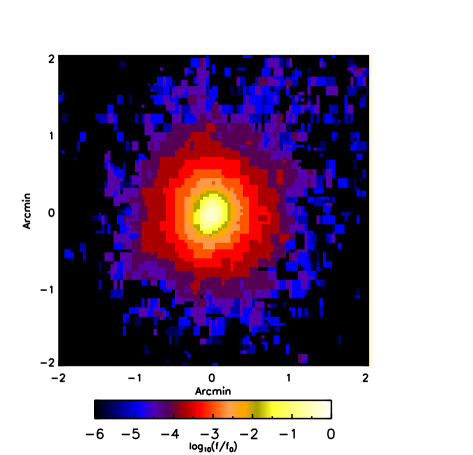
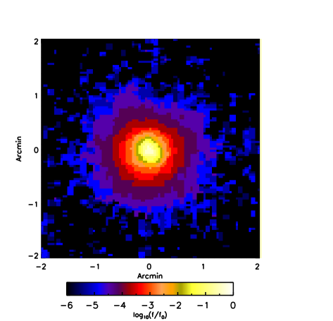
Figure 10.— The $1.1\,\mu$m (left) and $1.6\,\mu$m (right) Imager PSFs measured using stacked flight images from a combination of bright and faint sources as described in the text. The Imager PSF has a bright core with a faint extension to $r\sim 1^{\prime}$, and is circularly symmetric.

We synthesize the full PSF by matching the amplitudes of the core and extended PSFs in the overlap region, producing the smooth two dimensional PSF shown in Figure 10. The radial average of this full PSF is shown in Figure 11 and highlights that the core PSF is consistent with the laboratory focus data. However, the extended PSF deviates significantly from this approximation and is better described by a Voigt profile shape, characteristic of scattering in the optical components.

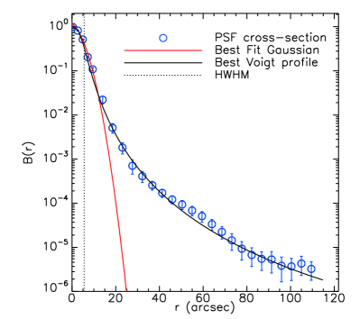
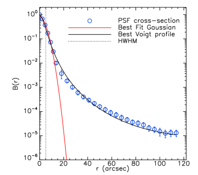
Figure 11.— The radial profile of the $1.1\,\mu$m (left) and $1.6\,\mu$m (right) Imager flight PSFs from Figure 10 (blue circles). The red curve shows the best fit Gaussian to the PSF core, while the black curve shows a best fit Voigt (i.e. the convolution of a Gaussian and Lorentzian) function to the extended PSF. This is indicative of scattering in the optical components. Finally, the black dash-dotted line shows the HWHM of the PSF, which matches the value measured in the laboratory.

The extended PSF is essential for determining the appropriate mask to apply for bright sources. The diameter of the PSF mask is adjusted based on the brightness of the source, and pixels above a given flux are cut. The cut is calculated by simulating all sources in either the 2MASS or Spitzer-NDWFS catalogs using their known fluxes and the Imager PSF. The cut mask is generated by finding all points on this simulation with fluxes $>3.3\,$nW/m²/sr and $1.8\,$nW/m²/sr at $1.1$ and $1.6\,\mu$m, respectively. This masking algorithm retains $\sim 50\,$% of the pixels for a cutoff of $18$ Vega mag, and $\sim$30% of the pixels for a cutoff of $20$ Vega mag. To test the cutoff threshold, we simulate an image of stars and galaxies and find that, cutting to $20$ mag, the residual spatial power from masked sources is $<8\times 10^{-2}\,nW^{2}m^{-4}sr^{-2}$ at $\ell=10^{4}$, comparable to the instrument sensitivity shown in Figure 7.

3.5. Off-axis response

The Imagers must have negligible response to bright off-axis sources, including the ambient-temperature rocket skin and shutter door, and the Earth. As described in Zemcov et al. (2012), we added an extendable baffle to eliminate thermal emission from the rocket skin and experiment door, heated during ascent by air friction, from illuminating the inside of the Imager baffle tube and scattering to the focal plane.

We measured the off-axis response of the full baffle system following the methodology in Bock et al. (1995). We replaced the Hawaii-1 focal plane array with a single optical photo diode detector and measured the response to a distant chopped source (see Tsumura et al. 2012 for a complete treatment of the measurement). The telescope gain function,

$$g(\theta)=\frac{4\pi}{\Omega}G(\theta),$$ (1)

where $\Omega$ is the solid angle of the detector and $G(\theta)$ is the normalized response to a point source is the quantity of interest for immunity to off-axis sources in surface brightness measurements (Page et al. 2003) and is independent of the optical field of view. The gain function was measured for three baffle configurations and is shown in Figure 12. The improvement from blackening the baffle tube and adding an extendable baffle section is notable for angles $\theta>20^{\circ}$. The stray light level from the Earth is given by

$$I_{\mathrm{stray}}=\frac{1}{4\pi}\int g(\theta)I_{\earth}(\theta,\phi)d\Omega,$$ (2)

where $I_{\earth}$ is the surface brightness of the Earth, and $I_{\mathrm{stray}}$ is the apparent surface brightness of stray light referred to the sky. Following the calculation described in Tsumura et al. (2012), we estimate that during the second flight CIBER observations of the fields listed in Table 1, where the Earth’s limb is $>72^{\circ}$ off-axis, the stray light level is calculated to be $2\,$nW/m²/sr and $1\,$nW/m²/sr in the $1.6$ and $1.1\,\mu$m channels, respectively.

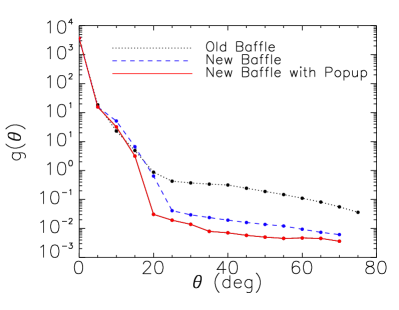
Figure 12.— The Imager telescope gain function, measured with the anodized fixed black baffle tube used in the first flight (dotted black line), an improved fixed baffle tube with a better laser black optical coating (Epner Technology Inc., dashed blue line), and the combination of the improved fixed baffle with an extendable baffle used in the second flight (solid red line). Details of the optical baffling can be found in Zemcov et al. (2012).

This level of stray light is quite small but not completely negligible, and potentially problematic in an anisotropy measurement depending on its morphology over the field of view. To quantify how stray light affects our measurements, we calculated the spatial power spectrum of the difference between two images, BoötesA - BoötesB which are separated by only $2^{\circ}$ on the sky and taken at nearly the same Earth limb avoidance angle, and BoötesA - NEP, from second flight data (see section 5). We find that the power spectra of these differences are the same to within statistical noise, and that the spatial fluctuations of the stray light signal are negligible.

We plan to observe these fields again in future flights at different Earth limb avoidance angles, including angles greater than $90^{\circ}$. The cross-correlation of such images from different flights is highly immune to residual stray light.

3.6. Flat Field Response

The instrumental flat field, which is the relative response of each detector pixel to a uniform illumination at the telescope aperture, is determined in flight by averaging observations of independent fields. Additionally, the flat field can be independently measured in the laboratory before and after flight as a check for systematic error. The laboratory flat field response is measured by illuminating the full aperture of a camera with the output of an integrating sphere. The sphere is illuminated with a quartz-tungsten halogen lamp which is filtered to produce an approximately solar spectrum at the output of the sphere, mimicking the spectrum of ZL.

The sphere was measured by the manufacturer to have uniformity as a function of angle to better than $5\times 10^{-3}$ over $10^{\circ}\times 10^{\circ}$. We scanned a small collimating telescope with a single pixel over the aperture, and determined that the sphere has angular uniformity to better than $1\times 10^{-3}$ over the $2^{\circ}\times 2^{\circ}$ Imager field of view. We also measured the spatial uniformity over the output port and saw no evidence of non-uniformity to $<7\times 10^{-3}$ over an 11 cm aperture.

To eliminate any effects from vacuum and thermal windows, we house the integrating sphere inside a vacuum chamber which mates to the front of the cryostat in place of the shutter door (see Zemcov et al. (2012) for details). Light is fed into the sphere from outside of the vacuum box so that the lamp can be chopped at the source, allowing us to remove the thermal background. An example flat field measurement for the $1.1\,\mu$m camera is shown in Figure 13.

The laboratory data are fitted over a limited period of the integration following array reset so as to avoid an appreciable error from non-linearity, as described in section 3.3, taking into account the minimum well depth of all pixels in the array. The instruments have a residual response to thermal infrared radiation in the laboratory with a typical photo current of $600\,e^{-}/s$ in the $1.6\,\mu$m array, which therefore limits the linear integration period to $\sim 5$ s. We obtained interleaved data with the source on and off to monitor and subtract this thermal background. After accounting for these effects, the final statistical accuracy of the laboratory flat field images shown in Figure 13 is $1.6\%$ per pixel. Laboratory flat fields were measured before and after the second flight to quantify the reproducibility of the lab flat field response. We binned $1.6\,\mu$m camera laboratory flat field images into 64 $(15\times 15)$ arcminute square patches in order to reduce statistical noise, and found the binned images agree to $<1\%(1\,\sigma$). The agreement between the flight and laboratory flat fields requires a full reduction of the flight data and will be presented in a future science paper.

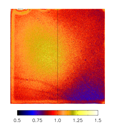
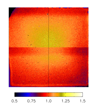
Figure 13.— The $1.1\,\mu$m and $1.6\,\mu$m Imager flat fields as measured in the lab using the apparatus described in Zemcov et al. (2012). The average response has been scaled to $1.0$ in this image, which shows the typical relative responsivity performance of the Hawaii-1 arrays in conjunction with the optics. The RMS variation in the pixel responsivities is $0.09$ at $1.1\,\mu$m and $0.12$ at $1.6\,\mu$m.

4. Modifications Following the First Flight

The Imagers were flown on the CIBER instrument on a Terrier Black Brant sounding rocket flight from White Sands Missile Range in 2009 February. Many aspects of the experiment worked well, including the focus, arrays and readout electronics, shutters, and calibration lamps. However, we also found several anomalies that led to modifications for subsequent flights.

4.1. Thermal Emission from the Rocket Skin

The instruments showed an elevated photon level during the flight due to thermal emission from the rocket skin, heated by air friction during ascent, scattering into the optics. The edge of the skin near the shutter door can directly view the first optic and the inside of the static baffle. This thermal response was pronounced at long wavelengths, as traced by the LRS (Tsumura et al., 2010). The $1.6\,\mu$m Imager was more affected by thermal emission than the $1.1\,\mu$m Imager, as expected from its longer wavelength response, giving 40 and 7 times the predicted photo current, respectively.

The measured thermal spectrum with the LRS should not produce a significant photo-current in the $1.1\,\mu$m Imager, as the band is supposed to cut off at $1.32\,\mu$m. The excess photo-current indicates the $1.1\,\mu$m Imager has some long wavelength response. The array response may continue somewhat beyond $2.5\,\mu$m, as the band-defining filters provided blocking out to just $2.5\,\mu$m and then open up. Also as with the NBS (Korngut et al., 2012) the filters may not attenuate scattered light at large incident angles as effectively as at normal incidence. The brightness observed by the $1.6\,\mu$m Imager is 6 times higher than the band-averaged LRS brightness. This could be due to a combination of the higher stray light response in the $1.6\,\mu$m Imager, and the filter blocking issues mentioned above. We installed an additional blocking filter providing $<0.1\%$ transmittance from $2.4\,\mu$m to $3.0\,\mu$m for both imagers.

We modified the front of the experiment section to better control the thermal and radiative environment at the telescope apertures. Most notably, we added extendable baffles to each of the instruments to eliminate all lines of sight from the skin to the optics or the inside surfaces of the baffle tubes. Zemcov et al. (2012) details the design of these baffles and the other changes made to the experiment section front end. Thermal emission is not detectable in the Imagers in the second flight, and is at least 100 times smaller than the first flight in the LRS data.

4.2. Rings and Ghosts from Bright Sources

During analysis of the first flight data, we discovered that bright objects outside of the Imager field of view create diffuse rings in the final images, as shown in Figure 14. Upon further analysis, we found that each of these rings was centered on a bright star outside the geometric field of view. The rings were caused by reflections off internal elements of the telescope assembly, as illustrated in Figure 15. There are two general classes of rings in the first flight images, though the second class contains two distinct populations; we denote these ring populations 1, 2 and 3 below. Table 3 gives details of the ring populations including their angular extent and coupling coefficients.

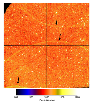
Figure 14.— $1.1\,\mu$m image of the Boötes A field from CIBER’s first flight showing rings which were later traced to reflections off components inside the Imagers, namely the lens mounts and instrument walls. As a guide the brightest rings are indicated with arrows. There are three separate populations of reflections which produce these rings. All sources which fall into their angular response regions will produce a ring, though only sources brighter than magnitude $\sim 4$ produce rings which are visible by eye. These rings produce excess power in the science power spectrum, but were eliminated by modifying the optics for the second flight.

Table 3First Flight Imager Ring Parameters.

Ring Type	$\theta_{\mathrm{min}}$	$\theta_{\mathrm{max}}$	$\int d\phi I_{\mathrm{ring}}(\phi)/\int I_{0}$
			Pre-fix	Post-fix ($3\sigma$)	Reduction in $C_{\ell}$
$1.1\mu$m Imager
1	$3.4^{\circ}$	$6.6^{\circ}$	$2.2\times 10^{-3}$	$<2.6\times 10^{-6}$	$>7\times 10^{5}$
2	$6.7^{\circ}$	$8.8^{\circ}$	$2.7\times 10^{-4}$	$<1.5\times 10^{-6}$	$>3\times 10^{4}$
3	$11.2^{\circ}$	$13.2^{\circ}$	$6.6\times 10^{-4}$	$<1.6\times 10^{-6}$	$>1\times 10^{5}$
$1.6\mu$m Imager
1	$3.4^{\circ}$	$6.6^{\circ}$	$4.1\times 10^{-3}$	$<3.0\times 10^{-6}$	$>1\times 10^{6}$
2	$6.7^{\circ}$	$8.8^{\circ}$	$3.5\times 10^{-4}$	$<1.9\times 10^{-6}$	$>3\times 10^{4}$
3	$11.2^{\circ}$	$13.2^{\circ}$	$1.3\times 10^{-3}$	$<4.3\times 10^{-6}$	$>9\times 10^{4}$

Population 1 rings are generated by reflections off a lens mounting flange (Figure 15), and are produced by bright sources between $3.4^{\circ}$ and $6.6^{\circ}$ off-axis. These rings also have the strongest optical coupling, with an integrated flux in the ring a few tenths of percent of the incident source flux. Given their large acceptance angle, stars brighter than $4^{\mathrm{th}}$ magnitude are sufficiently abundant to generate multiple bright rings.

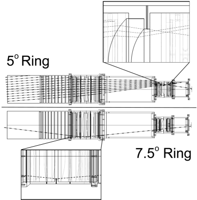
Figure 15.— Ray trace from an off-axis source which produces the rings observed at the focal plane. The first class of rings (labeled as $5^{\circ}$ in the Figure) are caused by glancing reflections off a flange supporting the back lens. The second class of rings (labeled as $7.5^{\circ}$) is produced by glancing reflections off flanges and lens holders in the front set of optics. For the second flight, these surfaces were cut back and grooved to reduce the glancing reflectance, removing the rings to a negligible level, as verified by laboratory measurements.

Following their discovery in the first flight data, we measured the population 1 rings and searched for other optical reflections in the laboratory. We illuminated each Imager aperture with collimated light and then scanned the angle of incidence of the collimated beam up to $25^{\circ}$ off-axis. The first set of measurements confirmed the existence of the population 1 rings, and allowed the discovery of the second class of fainter rings.

The second class of rings is comprised of two sub-populations which are both generated by reflections off the lens tube and lens support fixtures at the front of the optics assembly (Figure 15). These rings have flux coupling coefficients similar to, but slightly less than, the population 1 rings, but have much larger solid angles on the array and so produce smaller per pixel brightness. Together, population 2 and 3 rings are caused by bright sources $6.7^{\circ}$ to $13.2^{\circ}$ off-axis. These rings are not readily visible in the images from the first flight, though their presence was verified in the lab after flight.

Given the acceptance angles, star number counts and the quality of the ancillary data, the first set of rings are sufficiently bright to be modeled and masked from the first flight images. However, the second set of rings have a more complex morphology and fainter surface brightness, and are more difficult for us to confidently account for in the images.

To understand the systematic error associated with the population 2 and 3 rings, we modeled their effect by convolving the measured laboratory response with an off-axis star catalog for each field, and calculated the spatial power spectrum of the resulting images. These rings, if left unmasked, produce power above the instrument sensitivity level, as shown in Figure 16.

Figure 16.— Simulated power spectra for the second class of rings for both Imager instruments, $1.1\,\mu$m (left) and $1.6\,\mu$m (right). These spectra were computed given the ring parameters in Table 3 and the known star fluxes and positions near the CIBER fields. The instrument sensitivity is the the same as modeled in Figure 1. The amplitude of the power spectrum of the rings is different for each field because of the differing stellar populations near each, but similar between the bands because of the typical color of stars. For the second flight, the level of ring contamination is well below the instrument sensitivity, based on upper limits obtained in the laboratory following the modifications to the optics described in the text. The upper limit is shown for SWIRE, the most demanding field.

To remove the rings entirely, we made the optical simulation shown in Figure 15. Following characterization of the rings, the Imager optical assemblies were disassembled. The components responsible for the rings were grooved or cut back and re-anodized. The Imager optics were then reassembled, and the off-axis measurements were repeated. We did not observe any rings following these modifications. We place upper limits on the ring coupling factors shown in Table 3 which are based on the uncertainty in the integrated surface brightness over the nominal ring solid angles from the laboratory measurements. We propagated these upper limits through the model to produce synthetic images and then power spectra. The estimated reduction in the power spectrum from the first class of rings are given in Table 3. We find that the effect on the power spectrum is negligible compared with the instrument sensitivity after the optics modifications.

5. Instrument Performance from the Second Flight

The Imagers were flown on the CIBER instrument on a second sounding rocket flight in 2010 July. All aspects of the experiment performed well. We found no evidence of bright thermal emission from the rocket skin in either of the Imagers. We did not observe rings in the flight images. While the science data are still being analyzed, we summarize the observed brightness and array photo-currents in Table 4. Unfortunately, it is difficult to estimate the full in-flight sensitivity in the power spectrum without a noise estimator that accounts for correlated noise in the presence of sources and masking. Therefore we estimate the in-flight per-pixel sensitivities by evaluating the noise in the flight difference images (see Section 3.2). The corresponding per pixel surface brightness sensitivities, and point source sensitivities using a $2\times 2$ pixel aperture, are listed in Table 4. Our estimated sensitivity to the spatial power spectrum is shown in Figure 7 based on the variance of the power spectra of an ensemble of dark laboratory images combined with flight photon noise.

Table 4Calculated and Second Flight Sensitivities in a $50\,$s Observation.

	$1.1\,\mu$m Imager		$1.6\,\mu$m Imager
	Predicted	Achieved	Predicted	Achieved
Sky brightness	450	420	300	370	nW m-2 sr-1
Photo current	4.4	4.9	8.2	11.0	e${}^{-}/$s
Responsivity	10	11	28	31	me- s-1 / nW m-2 sr-1
Current Noise	0.31	0.35	0.41	0.45	e- s-1 ($1\sigma/$pix)
$\delta\lambda I_{\lambda}$	31.7	33.1	15.1	17.5	nW m-2 sr-1 ($1\sigma/$pix)
$\delta F_{\nu}$	18.5	18.4	18.2	17.8	Vega Mag $(3\sigma)$

We scale the photo currents in Table 4 to sky brightness units using a calibration based on point sources observed in flight. We stacked sources with flux between 16.0 and 16.1 Vega magnitudes in the 2MASS catalog and integrated over the stacked image to account for the extended PSF. We converted this point source calibration to surface brightness using the pixel solid angle, giving the calibration factors in Table 4.

6. Conclusions

We have designed and tested an imaging instrument optimized to search for the predicted spatial and spectral signatures of fluctuations from the epoch of reionization. The instrument demonstrates the sensitivity needed to detect, or place interesting limits upon, REBL fluctuations in the short observing time available in a sounding rocket flight. We have carried out a comprehensive laboratory characterization program to confirm the focus, characterize the flat field response, perform an end-to-end calibration, and measure the stray light response and detailed noise properties. After a first sounding rocket flight in 2009 February, we modified the instrument to eliminate response to thermal radiation from ambient portions of the payload, and to reduce stray light to bright stars outside of the field of view. Scientific data from the second flight in 2010 July are currently under analysis, and the instrument demonstrated sensitivity close to design expectations. The instrument characterization shows that systematic errors from the extended PSF, stray light, and correlated noise over the array are controlled sufficiently to allow a deep search for REBL spatial fluctuations. We recently completed a third flight in 2012 March that allows us to cross-correlate images at different seasons to directly assess any ZL fluctuations. The flight and recovery were successful, and a fourth flight is now planned. A successor instrument, with 3 or more simultaneous spectral bands and with higher sensitivity using a 30 cm telescope and improved Hawaii-2RG arrays, is currently in development.

7. Appendix

The calculated sensitivities in Table 4, Figure 1 and Figure 7 are based on a $50\,$s integration with the instrument parameters given in Table 2. The estimated photo current $i_{\mathrm{phot}}$ given by:

$$i_{\mathrm{phot}}\simeq\lambda I_{\lambda}\left(\frac{\eta A\Omega}{h\nu}\frac{\Delta\lambda}{\lambda}\right)\hskip 14.22636pt[\mathrm{e}^{-}/\mathrm{s}],$$ (3)

where $A\Omega$ is the pixel throughput, $\eta$ is the total efficiency, $\lambda I_{\lambda}$ is the sky intensity, and $\Delta\lambda$ is the integral bandwidth. The term in brackets in Equation 3 gives the surface brightness calibration from e${}^{-}/$s to nW/m²/sr. The current noise over an integration with continuous sampling is given by:

$$\delta i_{\mathrm{phot}}=\sqrt{\frac{i_{\mathrm{phot}}}{T}+\delta Q_{\mathrm{CDS}}^{2}\frac{6T_{0}}{T^{3}}}\hskip 14.22636pt[\mathrm{e}^{-}/\mathrm{s}],$$ (4)

where $\delta Q_{\mathrm{CDS}}$ is the correlated double sample read noise, $T=50\,$s is the integration time, and the frame rate $T_{0}=1.78\,$s. The surface brightness sensitivity is therefore:

$$\delta\lambda I_{\lambda}=\delta i_{\mathrm{phot}}\frac{h\nu}{A\Omega\eta\Delta\lambda/\lambda}\hskip 14.22636pt[\mathrm{nW\;m}^{-2}\;\mathrm{sr}^{-1}].$$ (5)

Finally, the point source sensitivity is given by:

$$\delta\lambda F_{\lambda}=\delta i_{\mathrm{phot}}\frac{\sqrt{N_{pix}}h\nu}{A\eta\Delta\lambda/\lambda}\hskip 14.22636pt[\mathrm{nW\;m}^{-2}],$$ (6)

where $N_{pix}$ is the effective number of pixels that must be combined to detect a point source, and we have assumed $N_{pix}=4$. These per-pixel sensitivities are used to estimate the sensitivity on the power spectrum in Figure 1 and Figure 7 using the formalism in Cooray et al. (2004). The calculation assumes the noise in each pixel is independent, and ignores errors from source removal and flat-field estimation.

References

- Abraham et al. (1997) Abraham, P., Leinert, C., & Lemke, D. 1997, A&A, 328, 702
- Adams & Skrutskie (1996) Adams, J., & Skrutskie, M. 1996, Airglow and 2MASS Survey Strategy, Tech. rep., University of Massschusetts
- Aharonian et al. (2006) Aharonian, F., et al. 2006, Nature, 440, 1018
- Allen (1976) Allen, C. W. 1976, Astrophysical Quantities, ed. Allen, C. W.
- Ashby et al. (2009) Ashby, M. L. N., et al. 2009, ApJ, 701, 428
- Berta et al. (2010) Berta, S., et al. 2010, A&A, 518, L30+
- Béthermin et al. (2010) Béthermin, M., Dole, H., Beelen, A., & Aussel, H. 2010, A&A, 512, A78+
- Biesiadzinski et al. (2011) Biesiadzinski, T., Lorenzon, W., Newman, R., Schubnell, M., Tarlé, G., & Weaverdyck, C. 2011, PASP, 123, 179
- Bock et al. (2006) Bock, J., et al. 2006, New Astronomy Review, 50, 215
- Bock et al. (1995) Bock, J. J., Lange, A. E., Onaka, T., Matsuhara, H., Matsumoto, T., & Sato, S. 1995, Appl. Opt., 34, 2268
- Bouwens et al. (2008) Bouwens, R. J., et al. 2008, ApJ, 686, 230
- Cambrésy et al. (2001) Cambrésy, L., Reach, W. T., Beichman, C. A., & Jarrett, T. H. 2001, ApJ, 555, 563
- Cooray et al. (2004) Cooray, A., Bock, J. J., Keating, B., Lange, A. E., & Matsumoto, T. 2004, ApJ, 606, 611
- Cooray et al. (2007) Cooray, A., et al. 2007, ApJ, 659, L91
- Cooray et al. (2012) Cooray, A., et al. 2012, ArXiv, 1205.2316
- Cutri et al. (2003) Cutri, R. M., et al. 2003, 2MASS All Sky Catalog of point sources., ed. Cutri, R. M., Skrutskie, M. F., van Dyk, S., Beichman, C. A., Carpenter, J. M., Chester, T., Cambresy, L., Evans, T., Fowler, J., Gizis, J., Howard, E., Huchra, J., Jarrett, T., Kopan, E. L., Kirkpatrick, J. D., Light, R. M., Marsh, K. A., McCallon, H., Schneider, S., Stiening, R., Sykes, M., Weinberg, M., Wheaton, W. A., Wheelock, S., & Zacarias, N.
- Dwek & Arendt (1998) Dwek, E., & Arendt, R. G. 1998, ApJ, 508, L9
- Dwek et al. (2005) Dwek, E., Krennrich, F., & Arendt, R. G. 2005, ApJ, 634, 155
- Essey & Kusenko (2010) Essey, W., & Kusenko, A. 2010, Astroparticle Physics, 33, 81
- Fazio et al. (2004) Fazio, G. G., et al. 2004, ApJS, 154, 10
- Fernandez et al. (2010) Fernandez, E. R., Komatsu, E., Iliev, I. T., & Shapiro, P. R. 2010, ApJ, 710, 1089
- Fixsen et al. (1998) Fixsen, D. J., Dwek, E., Mather, J. C., Bennett, C. L., & Shafer, R. A. 1998, ApJ, 508, 123
- Garnett & Forrest (1993) Garnett, J. D., & Forrest, W. J. 1993, in Society of Photo-Optical Instrumentation Engineers (SPIE) Conference Series, Vol. 1946, Society of Photo-Optical Instrumentation Engineers (SPIE) Conference Series, ed. A. M. Fowler, 395–404
- Gilmore (2001) Gilmore, R. C. 2011, ArXiv, 1109.0592
- Gonzalez et al. (2011) Gonzalez, A., et al. 2011, In Prep.
- González-Solares et al. (2011) González-Solares, E. A., et al. 2011, MNRAS, 416, 927
- Hauser et al. (1998) Hauser, M. G., et al. 1998, ApJ, 508, 25
- Helgason et al. (2012) Helgason, K., et al. 2012, ApJ, In Press
- Hwang et al. (2007) Hwang, N., et al. 2007, ApJS, 172, 583
- Jannuzi & Dey (1999) Jannuzi, B. T., & Dey, A. 1999, in Astronomical Society of the Pacific Conference Series, Vol. 191, Photometric Redshifts and the Detection of High Redshift Galaxies, ed. R. Weymann, L. Storrie-Lombardi, M. Sawicki, & R. Brunner, 111–+
- Jeon et al. (2010) Jeon, Y., Im, M., Ibrahimov, M., Lee, H. M., Lee, I., & Lee, M. G. 2010, ApJS, 190, 166
- Juvela et al. (2009) Juvela, M., Mattila, K., Lemke, D., Klaas, U., Leinert, C., & Kiss, C. 2009, A&A, 500, 763
- Kashlinsky et al. (2004) Kashlinsky, A., Arendt, R., Gardner, J. P., Mather, J. C., & Moseley, S. H. 2004, ApJ, 608, 1
- Kashlinsky et al. (2005) Kashlinsky, A., Arendt, R. G., Mather, J., & Moseley, S. H. 2005, Nature, 438, 45
- Kashlinsky et al. (2007) —. 2007, ApJ, 654, L5
- Kashlinsky & Odenwald (2000) Kashlinsky, A., & Odenwald, S. 2000, ApJ, 528, 74
- Keenan et al. (2010) Keenan, R. C., Barger, A. J., Cowie, L. L., & Wang, W.-H. 2010, ApJ, 723, 40
- Kelsall et al. (1998) Kelsall, T., et al. 1998, ApJ, 508, 44
- Knox (1995) Knox, L. 1995, Phys. Rev. D, 52, 4307
- Komatsu et al. (2011) Komatsu, E., et al. 2011, ApJS, 192, 18
- Lawrence et al. (2007) Lawrence, A., et al. 2007, MNRAS, 379, 1599
- Lee et al. (2009) Lee, H. M., et al. 2009, PASJ, 61, 375
- Levenson & Wright (2008) Levenson, L. R., & Wright, E. L. 2008, ApJ, 683, 585
- Levenson et al. (2007) Levenson, L. R., Wright, E. L., & Johnson, B. D. 2007, ApJ, 666, 34
- Lonsdale et al. (2003) Lonsdale, C. J., et al. 2003, PASP, 115, 897
- Madau & Pozzetti (2000) Madau, P., & Pozzetti, L. 2000, MNRAS, 312, L9
- Madau & Silk (2005) Madau, P., & Silk, J. 2005, MNRAS, 359, L37
- Marsden et al. (2009) Marsden, G., et al. 2009, ApJ, 707, 1729
- Matsumoto et al. (2005) Matsumoto, T., et al. 2005, ApJ, 626, 31
- Matsumoto et al. (2011) —. 2011, ApJ In Press
- Matsuura et al. (2011) Matsuura, S., et al. 2011, ApJ, 737, 2
- Moseley et al. (2010) Moseley, S. H., Arendt, R. G., Fixsen, D. J., Lindler, D., Loose, M., & Rauscher, B. J. 2010, in Society of Photo-Optical Instrumentation Engineers (SPIE) Conference Series, Vol. 7742, Society of Photo-Optical Instrumentation Engineers (SPIE) Conference Series
- Page et al. (2003) Page, L., et al. 2003, ApJ, 585, 566
- Pénin et al. (2011) Pénin, A., et al. 2011, ArXiv, 1110.0395
- Pyo & et al. (2011) Pyo, J., & et al. 2011, In Prep.
- Ramsay et al. (1992) Ramsay, S. K., Mountain, C. M., & Geballe, T. R. 1992, MNRAS, 259, 751
- Korngut et al. (2012) Korngut, P., et al. 2012, In Prep.
- Salvaterra et al. (2006) Salvaterra, R., Magliocchetti, M., Ferrara, A., & Schneider, R. 2006, MNRAS, 368, L6
- Salvaterra et al. (2011) Salvaterra, R., Ferrara, A., & Dayal, P. 2011, MNRAS, 414, 847
- Schroedter (2005) Schroedter, M. 2005, ApJ, 628, 617
- Skrutskie et al. (2006) Skrutskie, M. F., et al. 2006, AJ, 131, 1163
- Sullivan et al. (2007) Sullivan, I., et al. 2007, ApJ, 657, 37
- Thompson et al. (2007a) Thompson, R. I., Eisenstein, D., Fan, X., Rieke, M., & Kennicutt, R. C. 2007a, ApJ, 657, 669
- Thompson et al. (2007b) —. 2007b, ApJ, 666, 658
- Totani et al. (2001) Totani, T., Yoshii, Y., Iwamuro, F., Maihara, T., & Motohara, K. 2001, ApJ, 550, L137
- Tsumura et al. (2010) Tsumura, K., et al. 2010, ApJ, 719, 394
- Tsumura et al. (2012) —. 2012, ApJS, In Press
- Wright (2001) Wright, E. L. 2001, ApJ, 553, 538
- Yamamuro et al. (2006) Yamamuro, T., Sato, S., Zenno, T., Takeyama, N., Matsuhara, H., Maeda, I., & Matsueda, Y. 2006, Optical Engineering, 45, 083401
- Zemcov et al. (2012) Zemcov, M., et al. 2012, ApJS (In press)
- Zemcov et al. (2010) Zemcov, M., Blain, A., Halpern, M., & Levenson, L. 2010, ApJ, 721, 424