YSO jets in the Galactic Plane from UWISH2:
II - Outflow Luminosity and Length distributions in Serpens and Aquila

Abstract

Jets and outflows accompany the mass accretion process in protostars and young stellar objects. Using a large and unbiased sample, they can be used to study statistically the local feedback they provide and the typical mass accretion history. Here we analyse such a sample of Molecular Hydrogen emission line Objects in the Serpens and Aquila part of the Galactic Plane. Distances are measured by foreground star counts with an accuracy of 25 %. The resulting spacial distribution and outflow luminosities indicate that our objects sample the formation of intermediate mass objects. The outflows are unable to provide a sizeable fraction of energy and momentum to support, even locally, the turbulence levels in their surrounding molecular clouds. The fraction of parsec scale flows is one quarter and the typical dynamical jet age of the order of 10⁴ yrs. Groups of emission knots are ejected every 10³ yrs. This might indicate that low level accretion rate fluctuations and not FU-Ori type events are responsible for the episodic ejection of material. Better observational estimates of the FU-Ori duty cycle are needed.

1 Introduction

Star formation and in particular the mass accretion process is accompanied by the ejection of jets and outflows. These interact with the surrounding interstellar medium by shocks which excite, ionise or dissociate atoms and molecules. It is thought that these outflows provide localised feedback, i.e. they infuse energy and momentum into the ISM. In particular in low mass star forming regions where massive stars and their energetic radiation and winds are absent, they might be the governing mechanism to terminate further star formation (Walawender et al. (2005)). Thus, there are a number of ’small’ scale studies to characterise the population of outflows in nearby individual low mass star forming regions (e.g. Stanke (2001), Walawender et al. (2005), Hatchell et al. (2007), Davis et al. (2009), Khanzadyan et al. (2012)).

However, a large fraction, if not the majority of Galactic star formation is occurring in the presence of more massive stars and potentially in clusters along the Galactic Plane. We hence aim to characterise the general population of outflows from protostars and young stellar objects in an unbiased way. In order to have a representative sample of outflows which is free from selection effects we are conducting an unbiased search for jets and outflows in the Galactic Plane using the UKIRT Wide Field Infrared Survey for H₂ (UWISH2, Froebrich et al. (2011)). The sample of outflows from this survey will allow us to perform a statistical investigation of their properties and to address some of the open questions in the field such as: Why does a fraction of objects have no outflows, i.e. what triggers/stops outflow activity? Are the outflows related to FU-Ori type outbursts and if so how?

In this project, we focus our attention on the Serpens/Aquila region in Galactic plane, covered by UWISH2. In particular we investigate the area 18^∘ $<l<$ 30^∘, -1.5${}^{\circ}<b<$ +1.5^∘ which approximately covers 33 square degrees. In Ioannidis & Froebrich (2012) (Paper I hereafter) we presented the data (also discussed in Froebrich et al. (2011)) and discuss our detection method of jets/outflows and their potential driving sources. We did increase the sample of known Molecular Hydrogen emission-line Objects (MHOs) 15-fold and investigated their basic properties such as fluxes, apparent projected lengths and spatial distribution. We find that the flows tend to cluster in groups of a few (3 – 5) objects on scales of 5 pc, larger than typical young clusters. The scale height of the outflows with respect to the Galactic Plane is about 30 pc, similar to massive young stars.

In this paper we discuss in detail how we measure and calibrate the distance to the outflows in our sample (Sect. 2). In Sect. 3 we present our analysis, results and discussion. We re-evaluate the distribution of objects with respect to the Galactic Plane taking into account the measured distances. We then determine the statistically corrected luminosity functions and the associated star formation rate. We continue by presenting our investigation of the total jet energy and momentum input from our outflows into the interstellar medium. Furthermore, we analyse the outflow length distribution and the frequency of mass ejections.

In our forthcoming paper (Ioannidis & Froebrich, in preparation, hereafter Paper III), we will investigate in detail the driving sources and how their properties (e.g. luminosity, age, accretion rates) relate to the outflow parameters (e.g. luminosity, length).

2 Data analysis

2.1 Distance Determination

The determination of physical properties of the outflows, such as luminosity or length, requires us to know the distances to all objects in our sample. As has been shown in Paper I, the vast majority (above 90 %) of outflows in our sample are new discoveries. Thus, it is highly unlikely that we find objects with a known distance associated to all our objects. Even if we find literature distances to most of our objects, then they will most likely be measured by a mix of different methods – introducing biases. Finally, it is impractical to measure radial velocities for all objects (similar to the approach used in the Red MSX Source (RMS, MSX - Midcourse Space Experiment) survey by Urquhart et al. (2008) to determine distances. Only eight of our objects do actually coincide with RMS sources of known distance (they are indicated by a $+$ sign in the main result table in Appendix A). We thus require a way to determine the distances to all our objects in a homogeneous and unbiased way in order to obtain e.g. a statistically correct luminosity distribution.

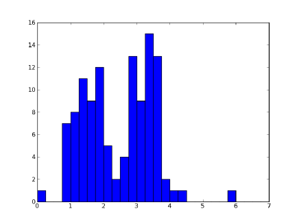
Figure 1: Distribution of the $J-K$ UKIDSS colour of stars near the Glimpse source G024.1838$+$00.1198, one of our calibration regions. One can clearly identify the separation of foreground and background stars at a value of $J-K=2.3$ mag.

We use the UKIDSS GPS near infrared JHK data (Lucas et al. (2008)) to determine the projected number density of foreground stars to the dark clouds associated with our jets and outflows. A similar approach has been used recently in Foster et al. (2012). They find that this extinction distance method agrees well with the maser parallax distances (within the errors) and is thus highly reliable. Similarly Froebrich & Ioannidis (2011) have used this method successfully to determine the distance to the cluster Mercer 14.

For each cloud with detected jets and outflows we perform the following: i) We select JHK photometry of the ’darkest’ part of the cloud to ensure that as few background stars as possible are included. The area selected has to be as large as possible to get a good reliable estimate of the number of foreground stars. ii) We plot a histogram of the $J-K$ colour of all selected stars and manually identify the break ($J-K$)_lim in the distribution caused by the cloud’s extinction. In Fig. 1 we show an example of the cloud near G024.1838+00.1198 (one of our calibration objects, see Sect. 2.2) for which we find ($J-K$)${}_{lim}=2.3$ mag. We consider the break to be real if at least 5 – 10 stars are apparently missing in one or more histogram bins. iii) We determine the projected foreground star density as the number of stars bluer than ($J-K$)_lim per unit area. Note that only stars above the local GPS completeness limit (determined as peak in the luminosity function for the stars selected within the cloud) in every filter are included. iv) We use the Besancon Galaxy model (Robin et al. (2003)) to determine out to which distance we should expect the same number of foreground stars per unit area with the local photometric limits. v) We estimate the distance uncertainty based on the uncertainty of the number $N$ of foreground stars used in each field ($\Delta N=\sqrt{N}$).

There are a number of MHOs (about 10 %) for which the described technique does not work successfully. In these cases the objects are not seen in projection onto an obvious dark foreground cloud. These outflows are either part of a very distant cloud or have formed in a low $A_{V}$ region. For all these objects the mean distance of all other outflows has been adopted in order to determine their luminosity and lengths. In Table LABEL:mainresults in Appendix A these MHOs are marked by a †. Note that they are not used in any of the statistical analysis of the luminosity and length distributions.

2.2 Distance Calibration

Our adopted distance determination method is a star counting technique in combination with a Galactic model. It has been used successfully by a number of authors, e.g. in Foster et al. (2012), Knude (2010), Froebrich & Ioannidis (2011). However, it is unclear if there are any systematic biases in applying this method. The Besancon model, for example, assumes a standard interstellar extinction law of 0.7 mag of $A_{V}$ per kpc distance (in agreement with the reddening towards old stellar clusters in the galactic disk; Froebrich et al. (2010)) which could be systematically different along our sight line leading to systematic shifts in the measured distances. Furthermore, the method will determine the distance to the first dark cloud along the line of sight. A fraction of our outflows could actually be situated at a larger distance, if a certain percentage of objects is situated along sight lines with overlapping clouds. We thus require to calibrate our distance calculation method with a sample of objects with known distances which are situated in dark clouds (similar to our sample), in order to establish the reliability and accuracy of the method. This calibration will not just be used to verify the method, but rather to estimate by which factor our distances are wrong for which fraction of objects. The RMS source list from Urquhart et al. (2008) has been selected for this purpose, as it represents the best available sample of objects associated with dark clouds, statistically distributed in a similar way to our outflows.

We selected all RMS sources within our survey area which have an estimated distance or (if there is a near/far ambiguity from the radial velocities) a near-distance between 2 kpc and 6.2 kpc. We then determine for each RMS source the distance in exactly the same way as for our outflows. There where a number of sources for which we could not measure a distance, since they did not coincide with an obvious dark cloud. These are most likely distant objects and we hence remove them from our sample. Note that they make up 10 % of the RMS objects and that we could not measure a distance for the same fraction of our outflows. In total we were able to determine the distance to 41 RMS sources in our survey area.

We perform a linear regression between our and the RMS distance which leads to the following calibration relation:

$$d^{cal,1}_{RMS}[kpc]=0.59\times d_{sc}[kpc]+1.97[kpc]$$ (1)

We denote with $d^{cal,1}_{RMS}$ calibrated distance of the RMS objects and with $d_{sc}$ the distance determined from foreground star counting and the Besancon Model. Note that we will refer to this as distance calibration method 1 throughout the paper. The root mean square ($rms$) standard deviation of this calibration is 1.0 kpc. We note that the scatter in the determined distances are not introduced by our determination of the ($J-K$)_lim values and the associated foreground star density. Expressed in units of the uncertainties of our distance errors, the deviations amount to eight standard deviations. Thus, the scatter is caused either by uncertainties in the RMS distances, large scale foreground clouds or low extinction (see discussion in Sect. 2.3). Note that Urquhart et al. (2008) quote an error of 1 kpc for their distances, based on peculiar motions of up to 10 km s^-1. This conservative estimate indicates that a large fraction of the scatter could be intrinsic to the RMS distances. Thus, our distances might be more accurate than implied by the $rms$-scatter, in agreement with the high accuracy found in Foster et al. (2012).

We construct a histogram of the logarithmic distance ratio $R=\log(d_{RMS}/d^{cal,1}_{RMS})$ with $d_{RMS}$ the distance in the RMS catalogue. This histogram has a width indicating a typical scatter of about 25 % for the distances.

Furthermore, we try to identify correlations of $d_{sc}$ with other outflow related parameters such as the galactic coordinates or the ($J-K$)_lim value used in the distance calculation. Only the Galactic Longitude $l$ shows a marginal correlation (correlation coefficient $r=0.41$). All other parameters have no systematic influence on the distance. If we hence consider the Galactic Longitude $l$ in the calibration we find the following calibration relation:

$$d^{cal,2}_{RMS}[kpc]=0.69\times d_{sc}[kpc]+0.16[kpc/deg]\times l[deg]-2.41[kpc]$$ (2)

Note that we refer to this as distance calibration method 2 throughout the paper. The $rms$-scatter of the distances using this calibration is 0.9 pc (six times the uncertainties of the individual measurements), slightly smaller than for calibration method 1. Including $l$ in the calibration leads to, on average, slightly higher distances and thus luminosities (and lengths) for our outflows, but the effect is marginal.

To summarise, we assume that the distances to the RMS calibration sources are accurate. Equations 1 and 2 are used to calibrate, in two ways, the distances estimated to each outflow using foreground star counts. These distances are listed in Table LABEL:mainresults in Appendix A.

2.3 Statistical Corrections

The above discussed distance calculation and calibration method shows to what extend our method over/underestimates distance to the RMS objects in our field. The distribution the logarithmic distance ratio $R$ essentially represents the probability distribution of the uncertainties in our distance determination (one for each calibration method). If $R$ is positive we underestimate the distance (e.g. due to foreground extinction/clouds), if $R$ is negative our distances are too large (e.g. caused by low $A_{V}$ clouds and hence the inclusion of blue background stars in the foreground star density). We now take the distribution of uncertainties for the measured distances to the outflows in the survey field is the same as for the calibration objects. This is justified, since most of the RMS objects are young stellar objects and are distributed in the same distance range and with the same scale height as our outflows (see Sect. 3.1 and 3.2).

Thus, in order to determine e.g. the luminosity distribution for the outflows, we add each outflow $N=10000$ times into the luminosity distribution. Each time the distance used in the calculation is the calibrated distance plus an uncertainty that is drawn from a sample of random numbers with the same distribution as $R$. Thus, we can determine statistically correct luminosity and length distributions for our outflows.

The luminosities are further influenced by interstellar and cloud extinction local to the outflow. Hence, we have to apply a further correction for each determined luminosity. Based on the distance for each object we use the standard 0.7 mag of optical extinction ($A_{V}^{d}$) per kpc distance from Froebrich et al. (2010). We further estimate the local or cloud extinction $A_{V}^{c}$ at the position of the outflow using the extinction maps by Rowles & Froebrich (2009). These maps give the total $A_{V}^{tot}$ along the line of sight and we take:

$$A_{V}^{tot}=A_{V}^{d}+A_{V}^{c}$$ (3)

We do of course not know where in the cloud the molecular hydrogen emission is situated (front or back). Note that the extinction values are low enough as to not introduce any bias towards outflows situated at the front of the clouds. Thus, for each of the $N$ times we add every outflow into the luminosity distribution (see above) we use an extinction of $A_{V}^{d}+w\times A_{V}^{c}$ where $w$ is a random number drawn from a homogeneous distribution between zero and one. All $A_{V}$ values are converted into K-band extinction (i.e. the extinction in the 1-0 S(1) line) using $A_{V}=9.3\times A_{K}$ following Mathis (1990).

In order to establish a statistically correct length distribution, we need to correct for the unknown inclination angle of the outflow. We find, however, that it is more convenient not to apply this correction, but rather try to simulate the projected length distribution since outflows almost perpendicular to the plane of the sky are missing in our sample (see later in Sect. 3.7).

3 Results and Discussion

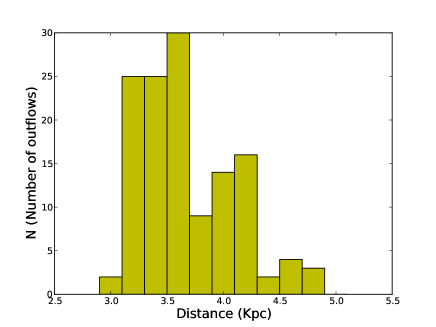
Figure 2: Distribution of distances of our outflows (using calibration method 1). There is a clear peak between 3.0 kpc and 3.5 kpc and a smaller, less obvious peak at about 4.2 kpc. Objects without determined distance are excluded.

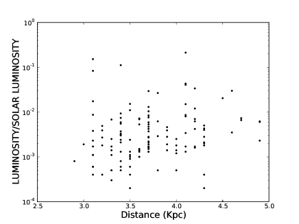
Figure 3: Outflow distances vs. H₂ 1-0 S(1) luminosities (based on calibration method 1). We detect outflows out to 5 kpc, and there is no clear trend in the diagram. Our estimated completeness limit for the outflow H₂ 1-0 S(1) luminosity within 5 kpc is 10^-3 L_⊙. The large number of objects at 3.7 kpc is due to the objects where we could not determine any distance and applied the mean distance.

3.1 Distance distribution

Since there are two calibration methods for the determined distance, we list both values in Table LABEL:mainresults in Appendix A. In general method 1 (simple calibration without considering the Galactic Longitude) gives slightly lower distances than method 2. A ${\dagger}$ symbol indicates outflows where we could not determine a distance and we used the mean distance measured for all other objects in those cases. Note that we exclude all these sources from any further statistical analysis.

The distances measured for our outflows are generally in the range from 2.0 kpc to 5.0 kpc. This is within the distance range of the RMS objects that are used for the calibration. The distribution of distances shows a peak at 3.0 – 3.5 kpc, indicating the presence of a spiral arm along this sight line. There is a second, less obvious peak at 4.2 kpc (see Fig. 2). In Urquhart et al. (2011) a similar increase in the number density of RMS sources in the same area can be seen at distances of about 3 – 4 kpc. The difference in the number of objects in both peaks is not due to completeness issues. The fraction of low luminosity outflows is the same for both (see Fig. 3). Thus, the more nearby feature has a larger number of active outflow driving sources.

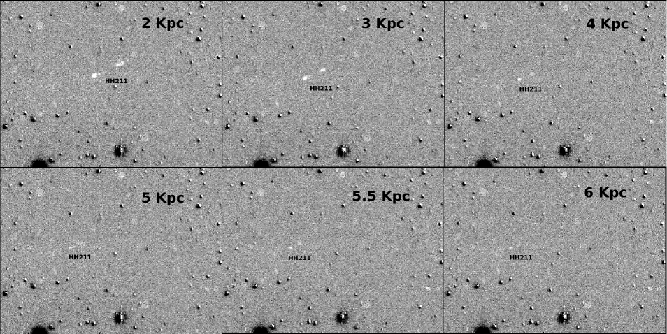
Figure 4: HH 211 as it would appear in one of our H₂ - K difference images at different distances (near the ’HH 211’ label). The well known object is placed flux calibrated and scaled in a relatively ’normal’ cloud region in one of our survey images. The small images are 80″ $\times$ 60″ in size and the distance of HH 211 are indicated in each panel. At distances at and above 5 kpc the outflow becomes indistinguishable from a very red or variable point source.

In order to estimate out to which distance we would in principle be able to detect molecular hydrogen outflows we used HH 211 as an example. This outflow is driven by a young Class 0 source and emits about 3.1 $\times$ 10^-3 L_⊙ in the 1-0 S(1) line of H₂ (Eislöffel et al. (2003)). We obtained a flux scaled image taken of this object in the 1-0 S(1) line from Eislöffel et al. (2003) and placed it scaled to different distances into one of our UWISH2 images (which represents a typical region). Note that we do not apply any extinction corrections to the flux. The result of the exercise is shown in Fig. 4. At distances below 5 kpc the outflow can easily be identified as bright extended emission with a clear bipolar structure. Several of our outflows (e.g. MHO 2256, 2289, 2292, 2441) have a similar appearance. At larger distances, however, the apparent size of the H₂ emission knots sinks below our spatial resolution and thus the brightness decreases significantly. Furthermore, the emission line knots will appear as red or variable point sources (which might remain in the H₂ - K difference images - see Paper I) and would thus most likely no be contained in our outflow sample, in particular if it was situated in a region higher foreground star density.

In Fig. 3 we plot the outflow distances vs. the luminosity in the 1-0 S(1) line of H₂ as measured by us. We see that low luminosity objects are sparse, but there is no real trend of the minimum detected luminosity with distance. Thus, based on Fig. 3 we conclude that our survey is complete to 5 kpc for objects with more than 10^-3 L_⊙ in the 1-0 S(1) line of H₂. This corresponds to HH 211 like outflows with about 1 mag of extinction in the K-band. The completeness limit is mostly set by the flux detection limit of 3 $\times$ 10^-18 W m^-2 (discussed in Paper I), since most our objects are extended up to a distance of 5 kpc.

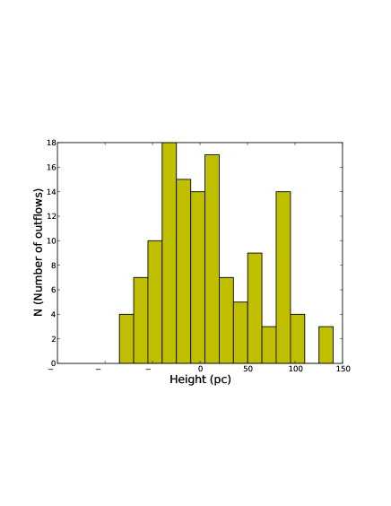
Figure 5: Distribution of the height above and below the Galactic Plane of our outflows (based on calibration method 1). The mean is shifted to about 20 pc below the Plane, and the width of the distribution shows a scale height of approximately 30 pc. Objects without distance determination are excluded.

3.2 Outflow scale height

With the distances for all outflows we are able to determine the distribution of objects with respect to the Galactic Plane. We already investigated this distribution in Paper I assuming a distance of 3 kpc for all outflows. As discussed above, most of our objects are indeed roughly at this distance, but the average is about 3.5 kpc. Thus, no significant change in the scale height compared to Paper I is expected. Only a small increase of 15 % should occur.

Figure 5 shows the height above and below the Galactic Plane for all outflows based on distance calibration method 1. The distribution is shifted to about 20 pc below the Galactic Plane indicating that in this region of the survey most star forming clouds are at negative galactic latitudes. The one sigma width of the distribution, or the scale height, is of the order of 30 pc. Hence our objects show the same distribution as typical massive OB stars (scale height about 30 – 50 pc, Reed (2000), Elias et al. (2006)) and the RMS sources in this area (Urquhart et al. (2011)). This justifies our use of the RMS sources as distance calibrators, since their distances and height distributions are the same as measured for our outflows. This in turn suggests that our outflows and massive star formation in the Galactic Plane are linked, even if only eight RMS objects coincide with any of our outflows (two of those might actually be background sources). In the forthcoming Paper III we will show that the driving sources for our outflows seem to be on average intermediate mass sources.

3.3 Driving source verification

The purpose of this paper is to investigate the luminosity and length distribution of the discovered outflows. Both rely on a correct as possible identification of the driving sources. This ’subjective’ task has been performed as described in Paper I. In order to ensure the correctness of the source identification we have repeated this task (half a year after it has been done originally) for all MHOs discovered in our field. For the vast majority of objects we have identified exactly the same objects as potential driving sources. Only for five out of the 134 MHOs did we select a different potential source.

We thus list in Appendix B and C the new properties and finding charts of the MHOs with a different source candidate (same as main tables in Paper I). In the light of these small changes we have re-done all the analysis from Paper I and there are no changes to any of the results and conclusions. We have also done all the analysis for this paper with both datasets and again, there are absolutely no differences in any of the results and conclusions.

3.4 Outflow luminosity function

The luminosities of our outflows (not corrected for extinction) in the 1-0 S(1) line of H₂ range from about 0.001 to 0.1 L_⊙, and depend slightly on the distance calibration method used. In Fig. 6 we show in a log-log plot the luminosity function for distance calibration method 1. The corresponding plot for method 2 and all other luminosity functions are summarised in Appenix D. All objects below the flux completeness limit and without properly determined distances are excluded.

The luminosity distribution represents a power-law of the form:

$$N\propto L_{1-0S(1)}^{\alpha}$$ (4)

with $\alpha$ in the range from -1.5 to -1.7, depending on the distance calibration method and histogram bin size.

When we apply our statistical distance correction to the luminosity distribution, we obtain the luminosity function as shown in Fig. 7. The statistical consideration of our distance uncertainties does influence the slope of the resulting luminosity function. It steepens the distribution, i.e. statistically our sample contains more low luminosity objects. The luminosity distributions for the distance calibration method 1 and 2 are also power-laws with slopes of $\alpha_{1}=-1.89$ and $\alpha_{2}=-1.88$, independent of the histogram bin width. Essentially, the two distributions are indistinguishable from each other. Thus, the shape of the luminosity distribution does not depend on the detailed way we calibrate our distance. Only the absolute values for the luminosities change slightly.

We finally apply the extinction correction based on the distance and the local cloud extinction. The resulting luminosity distributions are shown in Appendix D and are almost identical. The power-law slopes slightly increase to $\alpha_{1}=-1.93$ and $\alpha_{2}=-1.95$.

In summary, the number distribution of the 1-0 S(1) luminosities of our outflows can be represented by a power-law with a slope of $\alpha=-1.9$ with an uncertainty of about 0.1. This uncertainty accounts for possible changes of the slopes due to the extinction correction.

Based on some simple, statistically correct assumptions, we can investigate how such an outflow luminosity function can be interpreted. i) The total flux emitted by the outflow is ten times larger than the 1-0 S(1) flux. Hence the measured outflow luminosities are proportional to the total outflow luminosity emitted in all molecular hydrogen lines. This is correct for shocks at about 2000 K (Caratti o Garatti et al. (2006)), and has also been used by many other authors in statistical calculations (e.g. Stanke et al. (2002)); ii) Most of our outflows are driven by young protostars. The fact that we detect sources for only half the MHOs supports this fact. Furthermore, many sources are only detected at mid infrared wavelengths. We will present a detailed analysis of the source properties in Paper III, where we show that the driving sources are young embedded objects of intermediate mass.

Figure 6: 1-0 S(1) Luminosity distributions of our outflows for the distance calibration method 1. All objects with no measured distance are excluded, as are objects below the flux completeness limit. The fitted power law slope (about -0.5 to -0.7) is dependent on the histogram bin size due to the small number of objects.

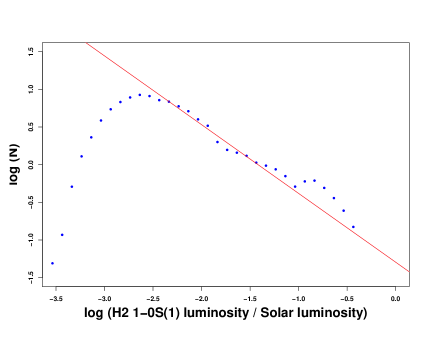
Figure 7: 1-0 S(1) Luminosity function of our outflows after we corrected for the statistical uncertainties in the distance by calibration method 1. Each outflow has been placed $N=10000$ times into the histogram (see text for details). All objects with no measured distance are excluded, as are objects below the flux completeness limit. The slopes for both calibration methods are indistinguishable and have a value of -0.9.

We can use the empiric relationship of the outflow H₂ luminosity and the bolometric driving source luminosity from Caratti o Garatti et al. (2006).

$$\log(L_{H_{2}})=0.58\times\log(L_{bol})-1.4.$$ (5)

Thus, we find for the distribution of the driving source bolometric luminosities:

$$N\propto L_{H_{2}}^{-1.9\pm 0.1}\propto L_{bol}^{-1.10\pm 0.05}$$ (6)

If all our sources are protostars, then $L_{bol}$ is dominated by the accretion luminosity $L_{acc}$ which scales like: $L_{acc}\propto\dot{M}MR^{-1}$. We can either use that the accreting central core has a constant density (then $R\propto M^{1/3}$ and thus $MR^{-1}\propto M^{2/3}$) or a constant radius (following Hosokawa et al. (2011) and thus $MR^{-1}\propto M$). For this range of possibilities the accretion luminosity will thus scale as $L_{acc}\propto\dot{M}M^{0.85\pm 0.15}$.

The mass accretion rate could scale as a power law with mass ($\dot{M}\propto M^{\beta}$). We observe each object at a time when it has accreted a fraction $X$ of its final mass, which statistically should be the same for all objects. Lastly, the distribution of final masses of the sources of our outflows should represent a Salpeter like mass function. Hence we find that

$$N\propto M^{-2.35}\propto M^{-(1.1\times\beta+0.95)\pm 0.20}$$ (7)

and thus $\beta=1.3\pm 0.2$. Which means that based on our outflow luminosity function, the average mass accretion rate for protostars scales like

$$\dot{M}\propto M^{1.3\pm 0.2}.$$ (8)

Finally, the accretion time scale $t_{acc}$ for an object of mass $M$ would scale like

$$t_{acc}\propto M^{-0.3\pm 0.2},$$ (9)

i.e. more massive stars spend less time accreting material. Note that these results have been determined based on a number of assumptions and hence might be slightly different in reality. However, based on our data we can certainly rule out that the average mass accretion rates for protostars driving our outflows is independent of the final stellar mass. Any further details such as the exact values and uncertainties of the inferred power law index should be investigated with more detailed numerical models able to link accretion rates, source and outflow luminosities (e.g. Smith (1998)).

If we would not correct our luminosity distribution for the distribution of uncertainties ($R$), then we would obtain $\beta=1.8$, an even stronger dependence of the average mass accretion rate on the final stellar mass.

We can also compare our result to the data from Stanke et al. (2002) who investigated the outflow luminosities in Orion A. There the 1-0 S(1) luminosities span a range from 10^-4 to 10^-2 L_⊙ and are hence one order of magnitude smaller on average than our values. The distribution of the L${}_{H_{2}}$ values is flatter than ours, with a value of $\alpha=-1.1$, which would lead (with the same assumptions as above) to $\beta=2.8$.

3.5 Star Formation Rate

When we convert our 1-0 S(1) luminosities into an H₂ luminosity (without accounting for extinction), our outflows cover a range of brightnesses from 0.01 L_⊙ to 1.0 L_⊙. This is in good agreement with the values for other molecular hydrogen outflows e.g. in Caratti o Garatti et al. (2008). In this paper one can also see that only very few objects are brighter than 1.0 L_⊙ and thus most of our outflows are driven by low and/or intermediate luminosity/mass protostars.

The total H₂ outflow luminosity of all objects in our investigated area is 9 L_⊙ or 12 L_⊙, depending on the distance calibration method. If we correct for extinction using $A_{K}=1$ mag (a typical value for the objects in our field), then the total H₂ luminosity in the survey area is 25 L_⊙, or 10 L_⊙/kpc².

With the assumptions from Sect. 3.4 (the outflow luminosity is linked to the accretion luminosity of the driving protostars as shown in Caratti o Garatti et al. (2008)) this converts into a total of 6 $\times$ 10⁴ L_⊙ of accretion luminosity. Note that this will be a lower limit, since there are some objects in Caratti o Garatti et al. (2008) which have much higher source luminosities compared to the general trend. If a typical protostar in our sample accretes onto a 2 M_⊙ intermediate mass core of 1.5 R_⊙ (Hosokawa et al. (2011)) then we can determine the total mass accretion rate in the survey area. If we normalise this to the area of 2.6 square kiloparsec we find a limit for the star formation rate ($SFR$) per square kiloparsec in the galactic disk.

$$SFR>2\times 10^{-3}M_{\odot}yr^{-1}kpc^{-2}$$ (10)

Our survey region covers an area roughly 4 – 7 kpc from the Galactic Centre. According to Boissier & Prantzos (1999) the star formation rate in the Milky Way ($SFR_{MW}$) drops significantly at galactocentric distances above 8 kpc. Thus, if we scale up our value to 200 square kiloparsec we find a limit of

$$SFR_{MW}>0.4M_{\odot}yr^{-1}$$ (11)

This is in agreement with recent estimates for the Galactic star formation rate e.g. by Robitaille & Whitney (2010) who found 0.7 – 1.5 M_⊙ yr^-1 based on the analysis of Spitzer detected young stellar objects. In Paper III we will estimate the properties of the driving sources in more detail, which will allow us to determine a more accurate limit for $SFR_{MW}$.

3.6 Outflow energetics

We can also investigate the total jet energy and momentum input from our outflows into the interstellar medium. As we have seen above, the typical object in our sample is a jet from a low and/or intermediate mass star. Furthermore, our data does not allow us to directly measure the jet power. We thus apply the method and generic values used in Davis et al. (2008) in order to get an order of magnitude estimate. Hence, we use $4\times 10^{37}$ J as the typical energy input of each jet and 1 M_⊙ km s^-1 as momentum input.

The turbulent energy in a cloud is approximately the cloud mass times the square of the turbulent velocity dispersion. For the latter we take 1 km s^-1 as a typical value, since the energy input from jets and outflows occurs usually locally (within at most a few parsec) from the star formation site, hence in regions where the turbulent velocities are not extremely high. Note that this value is also typical for nearby GMCs such as Perseus (Davis et al. (2008)).

Thus, the total energy input from our 130 outflows can provide enough turbulent energy for a total mass of just $2.5\times 10^{3}$ M_⊙. We can compare this to the total molecular gas mass within our survey region. According to Casoli et al. (1998) one expects about 3 M_⊙ pc^-2 of molecular gas (Boissier & Prantzos (1999) predict similar value of 6 M_⊙ pc^-2 at the galactocentric radius of our objects), which adds up to a total of 10⁷ M_⊙ in our survey area. However, as noted earlier, the energy input from the outflows will only occur locally, i.e. in the high density regions. These are most likely the parts of the cloud where the (column) density is above the star formation threshold. Rowles & Froebrich (2009) found that typically just one percent of a cloud is at these densities. Thus, only 10⁵ M_⊙ of cloud needs to be considered (this does not explain where the turbulent energy in the low column density regions originates).

In any case, the amount of mass that can be supported by the jets discovered in the survey area is a factor of 40 smaller than the actual mass at high densities. Thus, only if there are many generations of jets and outflows in each star forming region would they provide enough energy input to account for the turbulent energy. A typical age scatter of two million years would only allow ten generations of protostars. Thus, even locally, in the high density star forming fraction of the clouds, feedback from jets and outflows is insufficient as a source of the turbulent energy. Hence, high star formation rate regions like NGC 1333, which seem able to locally inject enough momentum to support the cloud (Walawender et al. (2005)) are not common in our survey area.

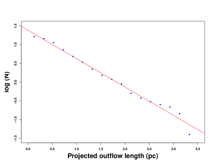
Figure 8: Statistically corrected distribution of the projected lengths of our outflows for the distance calibration method 1. Note that the distribution resembles an exponential and not a power law.

3.7 Outflow length distribution

The projected lengths have been calculated for all outflows with an identified driving source candidate. The lengths, derived using both distance calibration methods are listed in Table LABEL:mainresults in Appendix A. Note that we do not apply any corrections for single sided outflows, to allow a comparison to other works (e.g. Stanke et al. (2002), Davis et al. (2008), Davis et al. (2009)). We find a steep decrease in the number of flows with increasing length. In our sample we have between 15 % and 18 % of objects with a projected length above 1 pc (depending on the adopted distance calibration). If we apply a statistical correction of $4/\pi$ for a random distribution of inclination angles, then the fraction of parsec scale flows increases to about 25 %. Compared to other surveys the fractions of parsec scale flows (uncorrected for inclination) are: i) in Orion A Stanke et al. (2002) 8 %; ii) in Taurus, Auriga, Perseus Davis et al. (2008) 12 %; iii) in Orion A Davis et al. (2009) 9 %. Thus, since our survey traces more luminous outflows (see above), the fraction of parsec scale flows seems to be higher for brighter objects.

In Fig. 8 we show the distribution of the projected jet/outflow lengths in our sample. The plot is corrected for our statistical uncertainties in the distance calculations for method 1. However, both distributions are extremely similar and show an exponential decrease in the number of objects with increasing length and not a power law behaviour. The slope in the diagram hence indicates that the number $N$ of outflows is related to the flow length in the following way:

$$N\propto 10^{-0.75\times lenght[pc]}$$ (12)

We have run some simple simulations in order to understand the observed projected lengths distribution. As already stated in Paper I, simply assuming all jets are of the same length and randomly orientated should result in a completely different distribution (more larger than shorter flows up to a maximum projected length). A model of randomly orientated jets with uniformly distributed ages and a constant velocity fails to reproduce the data, in the same way as using a constant age and uniformly distributed velocities.

We therefore developed a family of models based on jets with different ages, homogeneously distributed between a minimum $a_{min}$ and maximum $a_{max}$. Furthermore, the jet velocities also range from a minimum $v_{min}$ to maximum $v_{max}$ value which are homogeneously distributed. Finally, the outflow inclination angle (angle between the jet axis and the line of sight) ranges from a minimum $i_{min}$ to 90^∘.

We then generated 16000 samples of 68 jets (the same number as jet lengths in our data), with parameters selected randomly from the following ranges:

$1000yrs\leq a_{min}\leq 5000yrs$

$10000yrs\leq a_{max}\leq 30000yrs$

$0km/s\leq v_{min}\leq 50km/s$

$90km/s\leq v_{max}\leq 150km/s$

$0^{\circ}\leq i_{min}\leq 50^{\circ}$

Note that these ranges of values for velocities and dynamical timescales/ages are in agreement with proper motion measurements e.g. from Davis et al. (2009) and Eislöffel et al. (1994). Each set of random projected length distributions was then compared via a Kolmogorov-Smirnov test with the observed distribution. This allowed us to determine the probability that the model distribution and the data are drawn from the same parent sample. When comparing the two length distributions based on the different distance calibration methods, we find that they agree with a 95 % probability. Any models that agree worse than 10 % with any of the data sets are considered bad.

We then investigate which models consistently lead to such a low agreement with the observations in order to exclude parameter values for the model. The best minimum inclination angle is about 20^∘. This shows that our sample typically does not contain many objects aligned perpendicular to the plane of the sky. Models with a lower minimum inclination angle generate too many short outflows, and models with a larger minimum inclination angle lack short objects.

The best fitting minimum/maximum velocity values are 40 km s^-1 – 130 km s^-1, while the age range of 4 –20 $\times$ 10³ yrs gives the best agreement with the data. These values lead to a range of jet lengths between 0.1 pc and 2.3 pc, in more or less the correct observed (exponentially decreasing) distribution. We note that these dynamical lifetimes are still at least an order of magnitude below estimates for protostellar lifetimes, which are typically a few 10⁵ yrs (Hatchell et al. (2007)).

The above parameter values imply that our sample does not contain very young and/or very slow moving jets. If they were very young they might have been missed as they are still deeply embedded and thus extincted. The same applies for the very slow moving jets, which additionally would lead to weaker shocks and thus less bright H₂ emission.

More detailed and realistic models should be tested against the available data. In particular the speed of the jet will change over time as energy and momentum is lost by radiation and entrainment of material. Any model should not just reproduce the length distribution but also the distribution of 1-0 S(1) luminosities and the relation between jet length and brightness (see below). However, only once the entire survey is analysed, will we have sufficient numbers of outflows to attempt this.

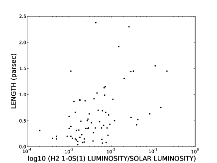
Figure 9: Projected outflow length against the outflow 1-0 S(1) luminosity based on the distance calibration method 1. Objects without determined distance are excluded.

3.8 Outflow length vs. luminosity

In Fig. 9 we plot the 1-0 S(1) luminosity against the projected outflow length. The plot demonstrates that the majority of the outflows is fainter than $10^{-2}$ L_⊙ and shorter than 1 pc in length. However, despite the poor statistics for bright outflows, there is a trend (corellation coefficient $r=0.47$) of increasing length with brightness. Essentially the bright outflows (L${}_{{\rm H}_{2}}>10^{-2}$ L_⊙) are on average about twice as long as the faint (L${}_{{\rm H}_{2}}<10^{-2}$ L_⊙) objects (1 pc vs. 0.5 pc).

Brighter integrated H₂ luminosities are indicative of higher surface brightness and/or larger shock area. The former will depend on a number of things such as shock velocity, ambient gas density, magnetic field strength/orientation, and ionization fraction (see e.g. Khanzadyan et al. (2004)). If the environment (clumpyness of the ISM surrounding the driving source) is the dominating factor for the outflow luminosity, then one might expect that shorter flows are brighter (the densest material is found closer to the star formation side), or that there is no correlation. Hence, Fig. 9 might indicate that brighter flows are generated by faster moving material since they are on average longer. This is also in line with the empiric relation of source luminosity and outflow luminosity from Caratti o Garatti et al. (2008) which should not exist if the environment plays a dominant role in determining the outflow brightness. However, as noted above for the length distribution, more realistic models need to be tested against the full survey data in the future.

Figure 10: Time difference between the emission of successive H₂ knots calculated based on the projected separation and an average speed of 80 km/s for the proper motion (using distance calibration method 1).

3.9 Mass ejection frequency

In our sample there are 29 outflows which have more than one H₂ emission knot on at least one side of the source. For these objects we are able to measure the projected distances between the emission knots and thus, with an average velocity, the time between the ejection episodes responsible for the knots. In total we have measured 76 distances between knots in our outflows. The resulting distributions of the ejection time differences are shown in Fig. 10. They are based on an average speed of 80 km s^-1 which is a typical speed for the jets and outflows in order to explain the length distribution (see above).

Similarly to the projected jet length distribution, we find a larger number of small distances between successive knots, or short times between the emission. With increasing time/distance between knots, the number of objects significantly decreases. There are, however, a few knots with large gaps between them, more than expected if the general decreasing trend is to continue.

With a velocity of 80 km s^-1 we find that the typical gaps between the knots corresponds to about 10³ yrs, while the largest time gaps are about 10⁴ yrs. This is a variation of roughly a factor of ten, with the largest time gaps reaching the typical dynamical jet lifetimes (see Sect. 3.7).

Note that we only included gaps between knots which could be clearly separated in our images (a few arcseconds – about 10³ yrs at a typical jet speed and a distance of 3 kpc). On smaller scales the knot-substructure is most likely caused or even dominated by the density structure of the ISM the jet is interacting with and not by the ejection history itself.

We tried to model the time gap distribution in the same manner as the jet lengths distribution (see Sect. 3.7). The same parameter ranges for the inclination and jet velocities are used. Instead of the jet age, we use a minimum $a_{min}$ and maximum $a_{max}$ age gap between the emission of successive knots.

$1000yrs\leq a_{min}\leq 3000yrs$

$3000yrs\leq a_{max}\leq 5000yrs$

Such a model is able to reproduce the general trend seen in Fig. 10, but contrary to the jet length distribution we do not find any model that agrees with the data above the 90 % level. This is most likely due to the increased number of objects with longer time gaps, which do not seem to follow the general trend. These large gaps can have a number of reasons: i) One of the knots does actually not belong to the outflow; ii) The knots are indeed emitted a long time apart; iii) We do not detect emission in between knots due to extinction and/or they are too faint. We also need to keep in mind that our model of constant velocity ejections is over simplistic, and the calculated ’time gaps’ between the knots are just an order of magnitude estimate.

However, we can assume that the separation of emission knots is related to episodes of increased mass accretion onto the central object. Numerical simulations (e.g. from Vorobyov & Basu (2006)) have shown how the mass accretion rate can vary over time in this ’burst-mode’ of star formation. These authors obtain significant peaks in the mass accretion rate which correspond to FU-Ori type outbursts. According to their models they occur about every 2 $\times$ 10⁴ yrs. In between the mass accretion rate varies less significant on timescales of about 1000 yrs. Our measured time differences hence correspond to those smaller accretion rate variations, while the total jet lifetime (as determined from the lengths distribution above) corresponds to the FU-Ori like eruption timescale.

Thus, our data are in agreement with model predictions if major episodes of mass accretion (such as FU-Ori outbursts) either trigger and/or stop the ejection of material in a protostellar jet. Lower level accretion rate increases occur on similar timescales as increased ejection of material in the jets (either density changes or velocity changes will lead to new emission knots forming). However, better statistics is required to be able to start trying to investigate how well our data matches with different models and FU-Ori timescales. Currently ongoing programs such as the VVV survey Minniti et al. (2010), the YSOVAR program (e.g. Morales-Calderón et al. (2011)) and others should soon be able to determine if the duty cycle of FU-Ori outbursts is 10³ or 10⁴ yrs with some certainty and what the frequency of accretion bursts of a given strength is.

If the larger value for the duty cycle is confirmed and FU-Ori bursts trigger a jet ejection phase, while subsequent smaller accretion bursts are responsible for continued emission knot formation, one would expect that statistically outflow driving sources should show enhanced mass accretion rates compared to a group of similar aged objects that do not drive outflows. We will test this by investigating the driving source properties of our sample and other YSOs in the same clouds in Paper III.

4 Conclusions

We used foreground star counts to molecular clouds associated with jets and outflows and a comparison to the Besancon Galaxy model by Robin et al. (2003) to determine their distances. To calibrate this method we utilised objects from the RMS survey by Urquhart et al. (2008) which are distributed in the Galactic Plane similar to our outflows. This method, together with the calibration allows us to estimate distances with a typical scatter of 25 %.

The majority of our detected outflows have a distance of about 3.5 kpc, indicating that the sight line crosses a spiral arm. The scale height of the outflows with respect to the Galactic Plane is 30 pc, of the same order as massive young stars. This is in agreement with the high outflow luminosities, and thus potential intermediate mass driving sources (Caratti o Garatti et al. (2006)) in our sample.

The outflow 1-0 S(1) luminosities range from slightly brighter than 0.1 L_⊙ to a few 10^-4 L_⊙, on average an order of magnitude brighter than in samples from nearby star forming regions. We estimate that our sample is complete for objects brighter than 10^-3 L_⊙ for distances of up to 5 kpc. This luminosity roughly corresponds to an HH 211 like object behind a K-band extinction of 1 mag.

The luminosity distribution of the outflows shows a power law behaviour with $N\propto L_{H_{2}}^{-1.9}$. With the assumption that 10 % of the H₂ flux is in the 1-0 S(1) line an using the empirical relation between the source bolometric (accretion) luminosity and the outflow luminosity this translates into a dependence of the average mass accretion rate on the final stellar mass of $\dot{M}\propto M^{1.3\pm 0.2}$. The total outflow luminosities also indicate a Milky Way star formation rate (averaged over a typical jet lifetime or the last 10⁴ yrs) of more than 0.4 M_⊙ yr^-1. Our sample of jets also indicates that they are not able to provide a sizeable fraction of the energy and momentum required to sustain the typical local levels of turbulence in their parental clouds.

The projected jet length drops exponentially in number for longer jets, and does not behave as a power law. The statistically corrected fraction of parsec scale flows is 25 %, almost twice as high as in typical nearby star forming regions. This is in agreement with our observed trend that more luminous outflows are longer and the fact that the average luminosity in our sample is higher than for outflow samples from e.g. Orion.

A simple Monte-Carlo type model of jets with speeds of 40 – 130 km s^-1 and ages between 4 – 20 $\times$ 10³ yrs can reproduce the observed length distribution. These lifetimes are an order of magnitude below estimates for the protostellar evolutionary phase. The model only fits the data if jets almost perpendicular to the plane of the sky are excluded.

Finally, we find that for typical outflow velocities the time gaps between the ejection of larger amounts of material (resulting in groups of emission features) are of the order of 10³ yrs. According to the burst mode of star formation models from e.g. Vorobyov & Basu (2006) the creation of the H₂ knots is hence linked to low level fluctuations of the mass accretion rate and not FU-Ori type events. Their duty cycle seems more in agreement with the total jet lifetime, which might suggest these outburst as trigger (or stopping point or both) of a jet ejection phase. However, better constraints of the FU-Ori duty cycle and mechanism as well as more detailed models are required to draw any further conclusions.

Appendix A MHO Properties Table

Table 1: Summary table of the MHO properties. In cases where several MHOs belong to the same outflow, the MHO number is labelled with an asterisk. Objects which coincide with a RMS source are labelled with a $+$ sign. We list the MHO number, the distance, the flux in the 1-0 S(1) line of H₂, the luminosity in the 1-0 S(1) line of H₂, the apparent and physical length. The numbers $1$ and $2$ indicate values determined using our two distance calibrations. $1$ includes the Galactic Longitude and $2$ does not. Objects where we could not determine a distance are indicated by †. In these cases we use the mean distance of all other objects to calculate luminosities and lengths.

	Dist.	Dist.	F[1-0 S(1)]	Lum.	Lum.	Apparent	Length	Length
MHO	2	1		2	1	length	2	1
	(Kpc)	(Kpc)	[10E-18 W/m2]	[Solar]	[Solar]	(arcsec)	(pc)	(pc)
MHO 2201∗	3.1	4.1	405.482	0.1212	0.2125	73	1.1	1.45
MHO 2212∗
MHO 2202+	3.1	4.1	77.481	0.0231	0.0406	21	0.32	0.42
MHO 2203	2.1	3.1	278.893	0.0379	0.0832	42	0.43	0.63
MHO 2204	2.1	3.1	509.659	0.0692	0.1520	50	0.51	0.75
MHO 2205	2.1	3.1	58.429	0.0080	0.0174	-	-	-
MHO 2206∗	3.4	3.4	304.384	0.1100	0.1115	93	1.54	1.55
MHO 2207∗
MHO 2208∗
MHO 2209	3.4	3.4	25.340	0.0092	0.0093	26	0.43	0.43
MHO 2210	3.4	3.4	20.150	0.0073	0.0074	40	0.66	0.66
MHO 2244	2.9	3.9	3.005	0.0008	0.0014	35	0.50	0.66
MHO 2245	2.1	3.1	12.587	0.0017	0.0038	18	0.18	0.27
MHO 2246	2.1	3.1	7.588	0.0010	0.0023	10	0.10	0.15
MHO 2247+	2.4	3.3	19.772	0.0035	0.0068	70	0.80	1.13
MHO 2248	2.1	3.1	3.800	0.0005	0.0011	26	0.26	0.39
MHO 2249	2.2	3.1	3.669	0.0005	0.0011	95	0.99	1.45
MHO 2250	4.3	4.9	8.288	0.0048	0.0062	29	0.61	0.69
MHO 2251+	4.3	4.9	3.033	0.0018	0.0023	4	0.08	0.09
MHO 2252	3.0	4.0	2.406	0.0007	0.0012	8.5	0.12	0.16
MHO 2253	4.0	4.7	10.497	0.0053	0.0073	-	-	-
MHO 2254	3.3	3.9	9.463	0.0032	0.0046	54	0.86	1.03
MHO 2255	3.5	4.0	1.058	0.0004	0.0005	10	0.17	0.20
MHO 2256	3.5	4.0	3.435	0.0013	0.0018	9	0.15	0.18
MHO 2257	3.5	4.0	4.862	0.0018	0.0025	18	0.3	0.35
MHO 2258	3.3	3.9	4.044	0.0014	0.0019	-	-	-
MHO 2259	2.6	3.3	7.424	0.0015	0.0025	-	-	-
MHO 2260	3.7	4.2	22.339	0.0098	0.0120	25	0.45	0.50
MHO 2261	3.7	4.2	62.588	0.0273	0.0337	72	1.31	1.45
MHO 2262+	4.7	4.7	9.502	0.0066	0.0066	18	0.41	0.41
MHO 2263	3.9	4.1	6.439	0.0031	0.0034	23	0.44	0.46
MHO 2264	3.9	4.1	15.185	0.0073	0.0080	18	0.34	0.36
MHO 2265	3.1	3.7	3.983	0.0012	0.0017	18	0.27	0.32
MHO 2266	3.4	3.9	5.976	0.0022	0.0028	28	0.46	0.53
MHO 2267	3.8	4.1	3.236	0.0015	0.0017	-	-	-
MHO 2268	4.4	4.5	0.108	0.0001	0.0001	-	-	-
MHO 2269+	4.3	4.5	32.477	0.0191	0.0204	60	1.27	1.31
MHO 2270	3.4	3.8	1.148	0.0004	0.0005	8	0.13	0.15
MHO 2271	3.4	3.8	6.578	0.0024	0.0029	19.5	0.33	0.36
MHO 2272	3.4	3.7	3.822	0.0014	0.0016	2.5	0.04	0.04
MHO 2273	4.0	4.1	2.535	0.0012	0.0013	-	-	-
MHO 2274	3.4	3.6	17.829	0.0065	0.0072	66	1.1	1.15
MHO 2275	3.4	3.6	17.181	0.0062	0.0069	-	-	-
MHO 2276	3.9	4.0	2.777	0.0013	0.0014	8	0.15	0.15
MHO 2277	3.6†	3.7†	24.144	0.0097	0.0104	-	-	-
MHO 2278	3.7†	3.7†	13.823	0.0058	0.0059	20	0.36	0.36
MHO 2279	4.3	4.2	3.023	0.0017	0.0016	5	0.1	0.10
MHO 2280∗	4.3	4.2	13.119	0.0074	0.0070	49	1.01	0.99
MHO 2281∗
MHO 2282	3.5	3.6	3.561	0.0014	0.0014	-	-	-
MHO 2283	3.5	3.6	2.511	0.0009	0.0010	20	0.33	0.35
MHO 2284+	3.5	3.6	3.745	0.0014	0.0015	18	0.3	0.31
MHO 2285	3.5	3.6	2.482	0.0009	0.0010	33	0.55	0.58
MHO 2286	3.4	3.6	13.093	0.0048	0.0053	-	-	-
MHO 2287	3.6	3.7	3.239	0.0013	0.0013	-	-	-
MHO 2288	3.6	3.7	10.087	0.0040	0.0042	-	-	-
MHO 2289	3.6	3.7	3.036	0.0012	0.0013	-	-	-
MHO 2290	3.6	3.7	12.735	0.0051	0.0053	27	0.47	0.48
MHO 2291	3.4	3.5	38.832	0.0144	0.0152	112	1.87	1.92
MHO 2292	5.3	4.9	7.950	0.0070	0.0060	6	0.16	0.14
MHO 2293	3.5	3.4	5.838	0.0022	0.0021	-	-	-
MHO 2294	3.5	3.4	1.553	0.0006	0.0006	-	-	-
MHO 2295	3.5	3.4	1.385	0.0005	0.0005	-	-	-
MHO 2296+	3.5	3.4	2.170	0.0008	0.0008	-	-	-
MHO 2297	3.3	3.2	1.326	0.0004	0.0004	10	0.16	0.16
MHO 2298	4.1†	3.7†	30.286	0.0156	0.0130	-	-	-
MHO 2299	3.0†	3.7†	4.781	0.0014	0.0021	-	-	-
MHO 2436	4.1†	3.7†	10.940	0.0057	0.0047	-	-	-
MHO 2437	4.5	4.1	28.685	0.0181	0.0150	-	-	-
MHO 2438	4.8	4.3	5.005	0.0036	0.0028	-	-	-
MHO 2439	4.1	3.7	5.294	0.0027	0.0022	-	-	-
MHO 2440	4.1	3.7	6.636	0.0034	0.0028	20	0.39	0.35
MHO 2441	4.1†	3.7†	19.608	0.0104	0.0084	12	0.24	0.22
MHO 2442	4.2	3.8	13.718	0.0076	0.0062	-	-	-
MHO 2443	4.9	4.3	7.008	0.0052	0.0040	-	-	-
MHO 2444	4.8	4.2	11.168	0.0080	0.0062	3.5	0.08	0.07
MHO 2445	4.8	4.3	3.482	0.0025	0.0020	11	0.26	0.23
MHO 2446	3.8	3.4	3.608	0.0016	0.0013	-	-	-
MHO 2447	3.8	3.4	6.586	0.0030	0.0024	-	-	-
MHO 2448	4.9	4.3	7.518	0.0056	0.0043	115	2.72	2.38
MHO 2449	4.9	4.3	3.770	0.0028	0.0021	4	0.09	0.08
MHO 2450	4.9	4.3	0.289	0.0002	0.0002	15	0.35	0.31
MHO 2451	4.9	4.3	8.806	0.0065	0.0050	-	-	-
MHO 2452	4.9	4.3	0.719	0.0005	0.0004	-	-	-
MHO 2453	4.9	4.3	3.087	0.0023	0.0018	43	1.01	0.89
MHO 2454	5.4	4.6	45.166	0.0403	0.0298	25	0.65	0.56
MHO 2455	5.4	4.6	5.353	0.0048	0.0035	-	-	-
MHO 2456	3.6†	3.7†	8.493	0.0035	0.0037	-	-	-
MHO 3200	3.0†	3.7†	68.260	0.0195	0.0294	80	1.18	1.44
MHO 3201	3.0†	3.7†	3.534	0.0010	0.0015	7	0.1	0.13
MHO 3202	3.6	3.5	6.238	0.0026	0.0024	51	0.9	0.88
MHO 3203	3.7	3.6	3.383	0.0015	0.0014	-	-	-
MHO 3204	3.7	3.6	3.304	0.0014	0.0013	50	0.91	0.87
MHO 3205	3.6	3.5	2.275	0.0009	0.0009	12	0.21	0.20
MHO 3206	3.3	3.3	3.439	0.0012	0.0011	-	-	-
MHO 3207	3.3	3.3	4.159	0.0014	0.0014	-	-	-
MHO 3208	3.3	3.3	1.440	0.0005	0.0005	-	-	-
MHO 3209	3.3	3.3	5.022	0.0017	0.0017	-	-	-
MHO 3210	3.6	3.5	2.853	0.0012	0.0011	12	0.21	0.20
MHO 3211	3.6	3.5	29.166	0.0117	0.0110	54	0.94	0.91
MHO 3212	3.6	3.5	2.527	0.0010	0.0010	-	-	-
MHO 3213	3.0	3.0	6.857	0.0019	0.0019	34	0.49	0.49
MHO 3214	3.9†	3.7†	6.214	0.0029	0.0027	28	0.53	0.50
MHO 3215	3.9†	3.7†	4.387	0.0021	0.0019	-	-	-
MHO 3216	3.1	4.1	82.356	0.0245	0.0432	26	0.39	0.52
MHO 3217	2.2	3.2	15.238	0.0022	0.0049	45	0.47	0.70
MHO 3218	2.2	3.2	5.549	0.0008	0.0018	58	0.61	0.90
MHO 3219	2.2	3.2	12.049	0.0017	0.0039	59	0.62	0.92
MHO 3220	2.2	3.2	8.344	0.0012	0.0027	-	-	-
MHO 3221	3.2	4.1	16.329	0.0053	0.0086	-	-	-
MHO 3222	2.5	3.4	10.380	0.0020	0.0037	6.5	0.08	0.11
MHO 3223	1.9	2.9	3.129	0.0004	0.0008	-	-	-
MHO 3224	2.6	3.5	1.700	0.0004	0.0006	-	-	-
MHO 3225	2.6	3.5	0.964	0.0002	0.0004	-	-	-
MHO 3226	2.6	3.5	3.466	0.0007	0.0013	-	-	-
MHO 3227	2.6	3.5	0.586	0.0001	0.0002	-	-	-
MHO 3228	2.0	3.1	2.092	0.0003	0.0006	-	-	-
MHO 3229	4.1	4.2	3.135	0.0017	0.0017	-	-	-
MHO 3230	2.0	3.1	5.628	0.0007	0.0017	-	-	-
MHO 3231	2.0	3.1	2.024	0.0002	0.0006	-	-	-
MHO 3232	2.0	3.1	1.201	0.0001	0.0004	-	-	-
MHO 3233	2.2	3.3	1.428	0.0002	0.0005	-	-	-
MHO 3234	3.1†	3.7†	3.940	0.0012	0.0017	-	-	-
MHO 3235	3.7	3.9	8.045	0.0034	0.0039	-	-	-
MHO 3236	2.9	3.3	0.913	0.0002	0.0003	-	-	-
MHO 3237	4.1	4.2	7.729	0.0041	0.0042	18	0.36	0.36
MHO 3238	3.2	3.4	8.895	0.0029	0.0033	-	-	-
MHO 3239	3.2	3.4	15.135	0.0049	0.0055	-	-	-
MHO 3240	3.6	3.8	60.245	0.0249	0.0266	126	2.22	2.30
MHO 3241	3.1	3.1	28.141	0.0083	0.0087	40	0.6	0.61
MHO 3242+	3.4	3.4	16.002	0.0058	0.0059	-	-	-
MHO 3243	3.4	3.4	8.172	0.0030	0.0030	38	0.63	0.63
MHO 3244	3.4	3.4	8.433	0.0030	0.0031	-	-	-
MHO 3246	3.1†	3.7†	17.575	0.0053	0.0076	4.5	0.07	0.08

Appendix B Corrected MHO Properties Table

Table 2: Properties of the five MHOs for which we identified a different driving source candidate compared to Paper I. An asterisk indicates MHOs which belong to the same outflow.

MHO	RA	DEC	F[1-0 S(1)]	Flux error	length	position angle	possible	source RA	source DEC
	(J2000)	(J2000)	[10E-18 W/m2]	[10E-18 W/m2]	(arcsec)	(degrees)	source	(J2000)	(J2000)
MHO 2271	18:35:31.7	-08:52:17	6.578	0.465	19.5	102	G023.2293-00.5289	18:35:30.4	-08:52:13
MHO 2272	18:35:51.3	-08:41:13	3.822	0.239	2.5	135	G023.4319-00.5212	18:35:51.4	-08:41:10
MHO 2276	18:35:22.9	-07:19:17	2.777	0.165	8	180	G024.5919+00.2119	18:35:22.9	-07:19:10
MHO 2280∗	18:38:55.4	-06:52:37	6.770	1.073	49	145	G025.3846-00.3724	18:38:56.5	-06:53:02
MHO 2281∗	18:38:57.3	-06:53:15	6.350	0.620	*	*	*	*	*

Appendix C Corrected MHO images

Table 3: Finding charts of the MHOs where we identified different driving sources compared to Paper I. An asterisk indicates MHOs which belong to the same outflow.

MHO	Image	Comments
MHO 2271		A faint bow shock like emission to the South East of candidate source Glimpse G023.2293-00.5289.
MHO 2272		Two compact knots with candidate source Glimpse G023.4319-00.5212 in the middle.
MHO 2276		A faint elongated emission knot South of candidate source Glimpse G024.5919+00.2119.
MHO 2280∗		A bright emission knot aligned with MHO 2281 and most likely driven by candidate source Glimpse G025.3846-00.3724.
MHO 2281∗		Extended bright, partly diffuse emission knot that is part of the same flow as MHO 2280 that is driven by candidate source Glimpse G025.3846-00.3724.

Appendix D Luminosity functions

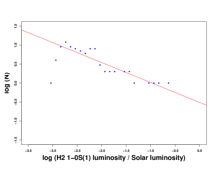
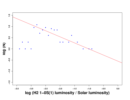
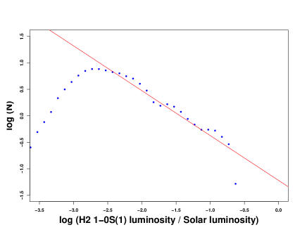
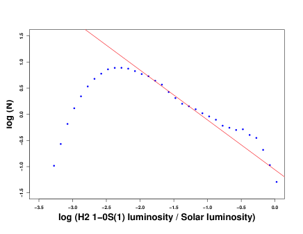
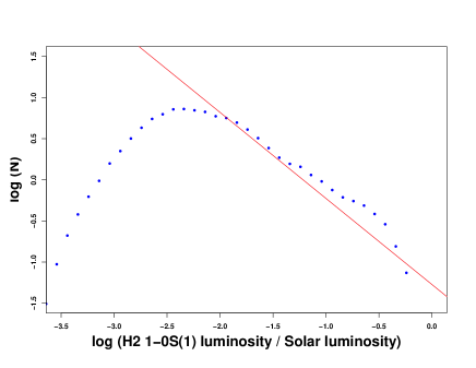
Figure 11: 1-0 S(1) Luminosity functions of our outflows. Top: Actual data; Middle: Statistically corrected for distance uncertainties; Bottom: Statistically corrected for distance uncertainties and extinction. The left column uses distance calibration method 1, the right column method 2. For the statistical correction each outflow has been placed $N=10000$ times into the histogram (see text for details). All objects with no measured distance are excluded, as are objects below the flux completeness limit. The slopes for the original data are -0.5 to -0.7, depending on the bin size. After the statistical correction the slopes are indistinguishable and have a value of -0.9.

References

- Boissier & Prantzos (1999) Boissier S., Prantzos N., 1999, MNRAS, 307, 857
- Caratti o Garatti et al. (2008) Caratti o Garatti A., Froebrich D., Eislöffel J., Giannini T., Nisini B., 2008, A&A, 485, 137
- Caratti o Garatti et al. (2006) Caratti o Garatti A., Giannini T., Nisini B., Lorenzetti D., 2006, A&A, 449, 1077
- Casoli et al. (1998) Casoli F., Sauty S., Gerin M., Boselli A., Fouque P., Braine J., Gavazzi G., Lequeux J., Dickey J., 1998, A&A, 331, 451
- Davis et al. (2009) Davis C. J., Froebrich D., Stanke T., Megeath S. T., Kumar M. S. N., Adamson A., Eislöffel J., Gredel R., Khanzadyan T., Lucas P., Smith M. D., Varricatt W. P., 2009, A&A, 496, 153
- Davis et al. (2008) Davis C. J., Scholz P., Lucas P., Smith M. D., Adamson A., 2008, MNRAS, 387, 954
- Eislöffel et al. (2003) Eislöffel J., Froebrich D., Stanke T., McCaughrean M. J., 2003, ApJ, 595, 259
- Eislöffel et al. (1994) Eislöffel J., Mundt R., Bohm K.-H., 1994, AJ, 108, 1042
- Elias et al. (2006) Elias F., Alfaro E. J., Cabrera-Caño J., 2006, AJ, 132, 1052
- Foster et al. (2012) Foster J. B., Stead J. J., Benjamin R. A., Hoare M. G., Jackson J. M., 2012, ApJ, 751, 157
- Froebrich et al. (2011) Froebrich D., Davis C. J., Ioannidis G., Gledhill T. M., Takami M., Chrysostomou A., Drew J., Eislöffel J., et al. 2011, MNRAS, 413, 480
- Froebrich & Ioannidis (2011) Froebrich D., Ioannidis G., 2011, MNRAS, 418, 1375
- Froebrich et al. (2010) Froebrich D., Schmeja S., Samuel D., Lucas P. W., 2010, MNRAS, 409, 1281
- Hatchell et al. (2007) Hatchell J., Fuller G. A., Richer J. S., 2007, A&A, 472, 187
- Hatchell et al. (2007) Hatchell J., Fuller G. A., Richer J. S., Harries T. J., Ladd E. F., 2007, A&A, 468, 1009
- Hosokawa et al. (2011) Hosokawa T., Offner S. S. R., Krumholz M. R., 2011, ApJ, 738, 140
- Ioannidis & Froebrich (2012) Ioannidis G., Froebrich D., 2012, MNRAS, 421, 3257
- Khanzadyan et al. (2012) Khanzadyan T., Davis C. J., Aspin C., Froebrich D., Smith M. D., Magakian T. Y., Movsessian T., Moriarty-Schieven G. H., Nikogossian E. H., Pyo T.-S., Beck T. L., 2012, ArXiv e-prints
- Khanzadyan et al. (2004) Khanzadyan T., Smith M. D., Davis C. J., Stanke T., 2004, A&A, 418, 163
- Knude (2010) Knude J., 2010, ArXiv e-prints
- Lucas et al. (2008) Lucas P. W., Hoare M. G., Longmore A., Schröder A. C., Davis C. J., Adamson A., Bandyopadhyay R. M., et al. 2008, MNRAS, 391, 136
- Mathis (1990) Mathis J. S., 1990, ARA&A, 28, 37
- Minniti et al. (2010) Minniti D., Lucas P. W., Emerson J. P., Saito R. K., Hempel M., Pietrukowicz P., Ahumada A. V., Alonso M. V., Alonso-Garcia J., Arias J. I., Bandyopadhyay R. M., 2010, New A, 15, 433
- Morales-Calderón et al. (2011) Morales-Calderón M., Stauffer J. R., Hillenbrand L. A., Gutermuth R., Song I., Rebull L. M., Plavchan P., Carpenter J. M., Whitney B. A., Covey K., Alves de Oliveira C., Winston E., McCaughrean M. J., Bouvier J., 2011, ApJ, 733, 50
- Reed (2000) Reed B. C., 2000, AJ, 120, 314
- Robin et al. (2003) Robin A. C., Reylé C., Derrière S., Picaud S., 2003, A&A, 409, 523
- Robitaille & Whitney (2010) Robitaille T. P., Whitney B. A., 2010, ApJ, 710, L11
- Rowles & Froebrich (2009) Rowles J., Froebrich D., 2009, MNRAS, 395, 1640
- Smith (1998) Smith M. D., 1998, Ap&SS, 261, 169
- Stanke (2001) Stanke T., 2001, PhD thesis, Universität Potsdam
- Stanke et al. (2002) Stanke T., McCaughrean M. J., Zinnecker H., 2002, A&A, 392, 239
- Urquhart et al. (2008) Urquhart J. S., Busfield A. L., Hoare M. G., Lumsden S. L., Oudmaijer R. D., Moore T. J. T., Gibb A. G., Purcell C. R., Burton M. G., Maréchal L. J. L., Jiang Z., Wang M., 2008, A&A, 487, 253
- Urquhart et al. (2011) Urquhart J. S., Moore T. J. T., Hoare M. G., Lumsden S. L., Oudmaijer R. D., Rathborne J. M., Mottram J. C., Davies B., Stead J. J., 2011, MNRAS, 410, 1237
- Vorobyov & Basu (2006) Vorobyov E. I., Basu S., 2006, ApJ, 650, 956
- Walawender et al. (2005) Walawender J., Bally J., Reipurth B., 2005, AJ, 129, 2308