Bosonic t-J model in a stacked triangular lattice and its phase diagram

Abstract

In this paper, we study phase diagram of a system of two-component hard-core bosons with nearest-neighbor (NN) pseudo-spin antiferromagnetic (AF) interactions in a stacked triangular lattice. Hamiltonian of the system contains three parameters one of which is the hopping amplitude $t$ between NN sites, and the other two are the NN pseudo-spin exchange interaction $J$ and the one that measures anisotropy of pseudo-spin interactions. Physical states of the system are restricted to the ones without the doubly-occupied state at each site. We investigate the system by means of the Monte-Carlo simulations and clarify the low-temperature phase diagram. In particular, we are interested in how the competing orders, i.e., AF order and superfluidity, are realized, and also whether supersolid forms as a result of hole doping into the state of the $\sqrt{3}\times\sqrt{3}$ pseudo-spin pattern with the $120^{o}$ structure.

1 Introduction

Study of systems in which competing orders coexist has been one of the most interesting topics in condensed matter physics. Among them, recent experiments on ⁴He under pressure have led to renewed interest of supersolid[1]. Also the search for a lattice supersolid has been motivated by the realization of optical lattices in ultracold atomic systems. As dimensionality and interactions between particles are highly controllable and also there are no effects of impurities, cold atomic system in an optical lattice is sometimes regarded as a “final simulator” for quantum many-body systems[2]. Numerical studies of hard-core bosons on a triangular lattice find that stable supersolid states form on doping of holes away from a $1/3$-filled solid ($2/3$-filled solid) with the $\sqrt{3}\times\sqrt{3}$ pattern[3, 4]. This provides example of old idea[5] that a finite density of defects in the solid (vacancies or interstitials) may Bose condense and form a superfluid in the existing crystalline background. In this paper we shall pursue the possibility of realization of “vacancy condensation” phenomenon[6] in boson systems in a triangular lattice in which a frustration exists.

The model that we study in this paper is a system of two-component hard-core bosons with nearest-neighbor (NN) pseudo-spin antiferromagnetic (AF) interactions in a stacked triangular lattice. The particle number at each site is less than unity, and therefore the model is sometimes called bosonic t-J model[7], i.e., a bosonic counterpart of the fermionic t-J model for the strongly correlated electron systems. The bosonic t-J model on a square lattice was originally studied as an effective model of the Bose-Hubbard model with strong on-site repulsions, and its phase diagram was clarified. In this paper, we shall study the mode on a stacked triangular lattice.

This paper is organized as follows. In Sec.2, we shall introduce the bosonic t-J model and explain its path-integral formalism for the numerical investigation. In order to incorporate the local constraint faithfully, we introduce a slave-particle representation. In Sec.3, we shall show results of the numerical study including phase diagrams, various correlation functions, and snapshots. We find that the system has a rich phase structure. Physical meanings of the results is discussed by using, e.g., a mean-field theory like approximation. Section 4 is devoted for conclusion and discussion.

2 Model and path-integral formalism

The mode that we study in this paper is the bosonic t-J model[7] in a three-dimensional (3D) stacked triangular lattice whose Hamiltonian is given as follows,

$$H_{\rm tJ} = -\sum_{\langle i,j\rangle}t(a^{\dagger}_{i}a_{j}+b^{\dagger}_{i}b_{j}+\mbox{h.c.})+J_{z}\sum_{\langle i,j\rangle}S^{z}_{i}S^{z}_{j}$$ (1)

$$+J\sum_{\langle i,j\rangle}(S^{x}_{i}S^{x}_{j}+S^{y}_{i}S^{y}_{j}),$$

where $a^{\dagger}_{i}$ and $b^{\dagger}_{i}$ are hard-core boson creation operators at site $i$, pseudo-spin operator $\vec{S}_{i}={1\over 2}B^{\dagger}_{i}\vec{\sigma}B_{i}$ with $B_{i}=(a_{i},b_{i})^{t}$, $\vec{\sigma}$ are the Pauli spin matrices, and $\langle i,j\rangle$ denotes the nearest-neighbor (NN) sites in the 3D stacked triangular lattice. Physical Hilbert space of the system consists of states with total particle number at each site less than unity (the local constraint: $a^{\dagger}_{i}a_{i}+b^{\dagger}_{i}b_{i}\leq 1$). As we consider the 3D system, there exist finite-temperature ($T$) phase transitions in addition to “quantum phase transition”, which takes place as the parameters in $H_{\rm tJ}$ are varied. The system $H_{\rm tJ}$ might be derived as an effective model of Bose-Hubbard model that describes a cold atom system in an optical lattice[8, 9]. In this case, $J$ and $J_{z}$ are related to the intra-species and inter-species on-site repulsions, and $J<0$. In this paper we study the bosonic t-J model (1) with general interests and treat $J$ and $J_{z}$ as free parameters. We mostly consider the case $J_{z},\ J\geq 0$, i.e., the frustrated case because it is very interesting to see how the frustrated pseudo-spin state evolves as holes are doped. Relation between the geometrical frustration and the formation of supersolid was discussed previously for the hard-core bosons in a triangular lattice[3, 4].

In addition to its own theoretical interest, another motivation for studying the model (1) with the antiferromagnetic (AF) coupling is provided by its relation to the fermionic t-J model. Recently, the fermionic t-J model was studied by mapping it to a kind of bosonic t-J model by using a Chern-Simons gauge field[10]. The resultant bosonic model is closely related to the present model expressed by using the slave-particle expression given by Eq.(2) later on. In Ref.[10], the model was studied by a mean-field type approximation. Then numerical study of the model (1) and to obtain its “exact phase diagram” are important for understanding the phase diagram of the fermionic t-J model. Effects of the Chern-Simons gauge field will be discussed later on by comparing the obtained results in this paper and the phase diargam of the fermionic t-J mode on the triangular lattice[11]. Furthermore very recently, it was shown by the numerical link-cluster expansion that the Fermi-Hubbard and Bose-Hubbard models on the square lattice exhibit very similar behavior in the strong-coupling region[12]. Therefore we expect that the results of the present study gives an important insight into phase diagram of the fermionic t-J model on the triangular lattice.

In order to incorporate the local constraint faithfully, we use the following slave-particle representation,

$$a_{i}=\phi^{\dagger}_{i}\varphi_{1i},\;\;\;b_{i}=\phi^{\dagger}_{i}\varphi_{2i},$$ (2)

$$\Big{(}\phi^{\dagger}_{i}\phi_{i}+\varphi^{\dagger}_{1i}\varphi_{1i}+\varphi^{\dagger}_{2i}\varphi_{2i}-1\Big{)}|\mbox{phys}\rangle=0,$$ (3)

where $\phi_{i}$ is a boson operator that annihilates hole at site $i$, whereas $\varphi_{\sigma i}\ (\sigma=1,2)$ are bosons that represent the pseudo-spin degrees of freedom. $|\mbox{phys}\rangle$ is the physical state of the slave-particle Hilbert space. Then the partition function $Z$ at temperature $T$ is given as follows in the path-integral methods,

$$Z=\int[D\phi D\varphi_{1}D\varphi_{2}]e^{-\beta H_{\rm tJ}},$$ (4)

where $\beta=1/(k_{B}T)$, $H_{\rm tJ}$ is obtained by substituting the slave-particles representation (2) into Eq.(1), and the path integral is performed with satisfying the slave-particle constraint (3). The original path-integral representation of the partition function contains terms like $\bar{a}_{i}\partial_{\tau}a_{i}$, where $\bar{a}_{i}$ is the complex number corresponding to $a^{\dagger}_{i}$ and $\tau$ is the imaginary time. As we discussed in the previous papers[13] and also showed explicitly by the numerical studies on certain models[4, 14, 15], effect of non-zero Matsubara-frequency modes in the 3D system at finite temperature is mostly the renormalization of the critical temperature and then the partition function in Eq.(4) is a good approximation for studying phase diagram at finite-$T$. Furthermore, as the system in the 3D stacked lattice can be in a sense regarded as a sequence of the 2D system, its low-$T$ phase diagram is closely related to that of the 2D system at $T=0$. Therefore, it is expected that the low-$T$ phase diagram of the 3D system in the stacked lattice obtained from $Z$ in Eq.(4) is quite similar to that of the 2D system at $T=0$ as verified in the previously studied cases[4, 14, 15]. In other words, the spatial third direction perpendicular to the 2D lattices plays a role similar to the imaginary-time direction. More detailed discussion on the model (1) at $T=0$ will be given in a future publication. Furthermore, it should be remarked here that a closely related discussion on the appearance of a Lorentz-invariant critical theory was given for the quantum phase model and the existence of Higgs mode was predicted in a two-dimensional superfluid on an optical lattice[16].

3 Numerical study

We employ both the grand-canonical and canonical ensemble for the practical calculation. In the grand-canonical ensemble, the chemical potential term like $\mu\sum_{i}\phi^{\dagger}_{i}\phi_{i}$ is added to $H_{\rm tJ}$. On the other hand in the canonical ensemble, the path integral in Eq.(4) is evaluated by means of the Monte-Carlo simulations with keeping the average density of holes fixed. To show results of numerical study, it is convenient to introduce the following dimensionless parameters, $c_{J}=\beta J,\ c_{Jz}=\beta J_{z}$, $c_{t}=\beta t$ and $\alpha=J/J_{z}$. Therefore large $c_{J}\ (c_{Jz})$ and/or $c_{t}$ corresponds to low-$T$ region.

To study the phase diagram, we calculate the internal energy $E$ and the specific heat $C$ defined as

$$E=\frac{1}{N}\langle{H}_{tJ}\rangle,\;\;C=\frac{1}{N}\langle({H}_{tJ}-E)^{2}\rangle,$$ (5)

where $\ N\equiv L^{3}$ with the linear system size $L$. We performed calculation up to $L=30$, and for the simulations, we employ the standard Monte-Carlo Metropolis algorithm with local update[17]. The typical sweeps for measurement is $(30000\sim 50000)\times(10$ samples), and the acceptance ratio is $40\%\sim 50\%$. Errors are estimated from 10 samples with the jackknife methods. We also calculate the hole density $\rho=\langle\phi^{\dagger}_{i}\phi_{i}\rangle$, and correlation functions $G_{\rm xy}(i,j)=\langle(S^{x}_{i}S^{x}_{j}+S^{y}_{i}S^{y}_{j})\rangle$, $G_{\rm z}(i,j)=\langle S^{z}_{i}S^{z}_{j}\rangle$, and $G_{\rm S}(i,j)=\langle\vec{S}_{i}\cdot\vec{S}_{j}\rangle$. It easily verified $\vec{S}^{2}_{i}=(a^{\dagger}_{i}a_{i}+b^{\dagger}_{i}b_{i})^{2}$, and then the magnitude of the pseudo-spin is decreased by the doping of hole. On the other hand, boson correlation function $G_{\rm B}(i,j)=\langle B^{\dagger}_{i}B_{j}\rangle$ is used to see if a superfluid forms.

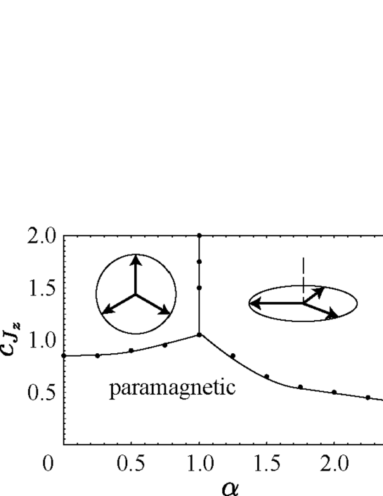
Figure 1: Phase diagram for anisotropic AF Heisenberg model in a stacked triangular lattice. Vertical axis plots $c_{Jz}$. At low $T$, there are two phases with a long-range order of 120^o pattern, which are separated with each other by the line $\alpha=1$ ($J=\alpha J_{z}$). Phase transitions from paramagnetic to ordered states are of second order, whereas that of $\alpha=1$ is called morphotropic phase boundary[19]. System size $L=24$ with the periodic boundary condition.

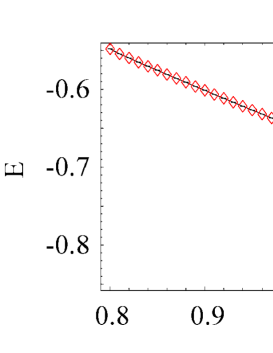
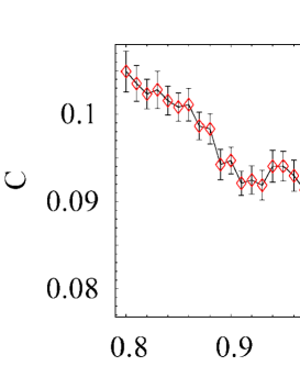
Figure 2: $E$ and $C$ as a function of $\alpha$ for $c_{Jz}=1.5$. At $\alpha=1$, $C$ does not have a peak but exhibits some peculiar behavior though $E$ indicates the existence of the phase transition. This is a typical behavior of the morphotropic phase boundary.

3.1 Anisotropic AF Heisenberg model on the stacked triangular lattice

At zero hole density, the system (1) reduces to the anisotropic AF Heisenberg model. The same model in the 2D triangular lattice has been studied rather intensively[18]. To identify the phase boundary of the present 3D model, $E$ and $C$ were calculated by the Monte-Carlo simulations. The spin correlation functions were also calculated in order to identify each phase. We show the obtained phase diagram in Fig.1. As $T$ is lowered, second-order phase transition from the paramagnetic phase to the spin-ordered states takes place. Specific heat $C$ exhibits a sharp peak at the transition points indicating the existence of the second-order phase transition. Location of the phase transition points is determined by the peaks of $C$. In the low-$T$ region, there are two phases separated with each other by the line $\alpha=1$.In the study of ferroelectric materials, the corresponding line is called the morphotropic phase boundary, and it plays an important role[19]. We show the internal energy $E$ and the specific heat $C$ as a function of the anisotropy $\alpha$ in Fig.2, which exhibit a “typical” behavior of the morphotropic phase boundary[9]. It should be remarked that the system has the $SU(2)$ pseudo-spin symmetry at $\alpha=1$, whereas $U(1)\times Z_{2}$ otherwise. This fact is the origin of the peculiar behavior of $E$ and $C$ at $\alpha=1$. The phase structure at low $T$, i.e., $c_{J},\ c_{Jz}\rightarrow$ large, is essentially the same with that of the 2D system at $T=0$, as it is expected from the above general consideration. We have also studied the correlations of spins in the vertical direction of the stacked triangular lattice, and found the strong AF long-range correlations in the two phased with the 120^o spin order and short-range one in the paramagnetic phase in Fig.1.

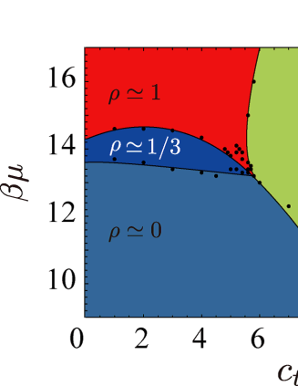
Figure 3: Phase diagram for bosonic t-J model in a stacked triangular lattice at low $T$, $c_{J}=6.0$ (grand-canonical ensemble). $\rho$ is hole density. Dots denote location of the phase transition observed by the numerical study. All phase transitions are of first order. SF stands for superfluid and this phase also has FM long-range order. The phase $\rho\simeq 0$ is essentially the pure spin system with the $\sqrt{3}\times\sqrt{3}$ symmetry and the phase with $\rho\simeq 1$ is the empty state. The phase with $\rho\simeq 1/3$ is explained in Fig.6. These three phases are all insulating.

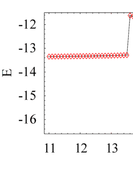
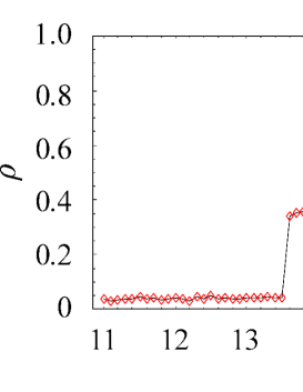
Figure 4: $E$ and $\rho$ as a function of $\mu$ with $c_{J}=6.0$ and $c_{t}=2.0$. There are two first-oder phase transitions. $L=30$.

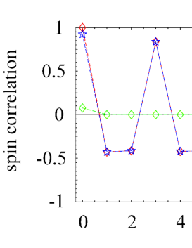
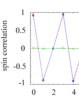
Figure 5: Spin correlation functions $G_{\rm S}(i,j),G_{\rm xy}(i,j)$ and $G_{\rm z}(i,j)$ for $c_{t}=2.0$ and $\beta\mu=12.0$ (left), $\beta\mu=14.0$ (right).

3.2 t-J_xy model

In this subsection, we focus on the $xy$ AF Heisenberg model by setting $J>0,\ J_{z}=0$ in Eq.(1) and study effect of the hole doping. The case of $J=0,\ J_{z}>0$ will be investigated in the subsequent subsection. For the ferromagnetic case $J<0$ and $|J|>|J_{z}|$, it is readily expected that the system has a similar phase diagram to that on the cubic lattice[9] as there are no frustrations in the system. One of the motivations to study the doped AF magnets on the triangular lattice comes from the possible spin liquid and superconductivity suggested by Anderson[20], and therefore we focus on the AF cases.

We first investigate the system in the grand-canonical ensemble. Obtained phase diagram in the $c_{t}-\beta\mu$ plane for $c_{J}=6.0$ is shown in Fig.3. For the region $c_{t}<5.5$, there exist three phases and they are separated by sharp first-oder phase transitions. See calculations of $E$ and the averaged hole density $\rho=\langle\phi^{\dagger}_{i}\phi_{i}\rangle$ in Fig.4, the both of which exhibit sharp discontinuities at $\beta\mu\simeq 13.5$ and $14.7$. From this observation, we judge the existence of the first-order phase transitions there. The location of the phase transition points is determined by $E$.

It is obvious that the phase for $\beta\mu<13.6$ is nothing but the pure spin system of very low hole density that has the long-range order of the three-sublattice $\sqrt{3}\times\sqrt{3}$ pattern. See the correlation function for $\beta\mu=12.0$ in Fig.5. On the other hand in the intermediate region $13.6<\beta\mu<14.4$, stable state with $\rho={1\over 3}$ is realized. Correlation functions in Fig.5 indicate that the state is nothing but the one shown by the snapshot in Fig.6. We verified this conclusion by calculating the hole density. For $\mu>14.4$ the density of hole is almost unity and the empty state forms there.

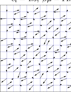
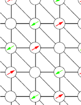
Figure 6: (Left) Snapshot for $c_{t}=4.5$ and $\beta\mu=14.0$. Holes are localized and a kind of AF configuration of pseudo-spin is realized. We show pseudo-spins in the $S^{x}-S^{y}$ plane for $S^{z}$ component is negligibly small. Therefore the length of arrows indicates magnitude of pseudo-spins. (Right) Caricature of typical configuration obtained by MC simulation.

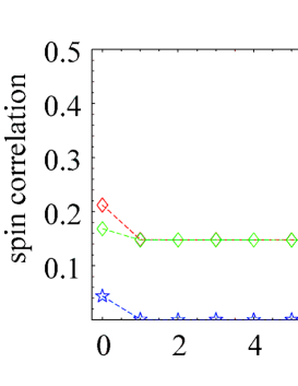
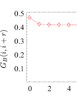
Figure 7: Spin (left) and boson (right) correlation functions for $c_{t}=12.0$ and $\beta\mu=11.0$

As $c_{t}$ is increased, all the above three phases make a phase transition to a new phase via first-order phase transitions. $E$ exhibits discontinuities at the phase boundary of the phase $\rho\simeq 0.5\sim 0.7$ in Fig.3, indicating first-order phase transitions. Hole density of this phase is $\rho\simeq 0.5-0.7$, and the calculated spin correlation indicates the existence of the ferromagnetic (FM) long-range orders $\langle S^{z}_{i}\rangle\neq 0$ and also non-vanishing superfluidity $\langle B_{i}\rangle\neq 0$. See Fig.7. This result means that the system is composed of, say, $a$ bosons and the Bose condensation of $a$ boson takes place there. If we impose the condition that the total number of $a$ boson and that of $b$ boson are equal, the phase separation to $a$-rich region and $b$-rich region is expected to occur. This problem is under study and result will be published in a near future.

In the grand-canonical ensemble, the most stable state in the system appears for each value of the chemical potential. Near the first-order phase transition, it is rather difficult to control the particle density by varying the value of the chemical potential. Then it is quite interesting to study the system in the canonical ensemble by keeping the hole density constant. In the present system, we focus on how the state of hole density, say, 40% evolves as the hopping parameter $t$ is increased.

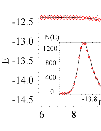
Figure 8: Internal energy $E$ as a function of $c_{t}$ for $\rho=0.4$ and $c_{J}=10.0$. At $c_{t}\simeq 13$, there exists a first-order phase transition. (Inset) $N(E)$ for $c_{t}=13.2$ exhibits the double-peak shape indicating the first-order phase transition.

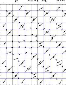
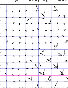
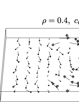
Figure 9: Snapshots for $\rho=0.4,\ c_{J}=10.0$ and $c_{t}=5.0$ (left), $c_{t}=15.0$ (center, right (oblique angle)). Left and center snapshots show $S^{x}-S^{y}$ component of pseudo-spin. Right one is snapshot from an oblique angle, and length of arrows indicates magnitude of pseudo-spins.

In Fig.8, we show the internal energy $E$ for $c_{J}=10.0$ as a function of $c_{t}$. We also measures the number of states $N(E)$, which is defined as $Z=\int dEN(E)\exp(-\beta E)$. The result indicates that there exist a first-order phase transition at $c_{t}=13.2$. In order to understand the physical meaning of the phase transition, it is quite useful to see snapshots of the two phases separated by the phase transition. See Fig.9. From the snapshot for $c_{t}=5$, it can be seen that the phase of $\rho={1\over 3}$ survives and there is a void of very low particle density as a result of an excess of holes compared to $\rho={1\over 3}$. On the other hand, the snapshot for $c_{t}=15$ shows that the phase separation takes place, i.e., the region of pure-spin phase with the $\sqrt{3}\times\sqrt{3}$ pattern and the region of the superfluid coexist, but they are immiscible. In the superfluid region, the boson has a nonvanishing expectation value $\langle B_{i}\rangle\neq 0$. The observation obtained through the snapshots is verified by the correlation functions $G_{\rm B}(i,j)$ shown in Fig.10.

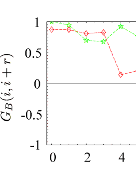
Figure 10: Boson correlation functions for $\rho=0.4$ and $c_{t}=15.0$ along the two lines shown in Fig.9.

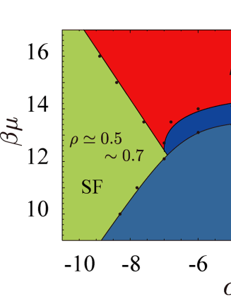
Figure 11: Phase diagram for $c_{t}<0$. There are four phases as in the case of $c_{t}>0$ and they are separated by first-order phase transition lines. Physical meaning of each phase is explained in the text.

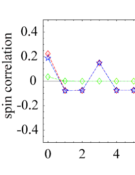
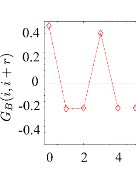
Figure 12: Spin (left) and boson (right) correlation functions for $c_{t}=-19.0$ and $\beta\mu=11.0$. The spin correlation function $G_{\rm xy}(i,j)$ exhibits the $\sqrt{3}\times\sqrt{3}$ pattern. The boson correlation $G_{\rm B}(i,j)$ also shows a similar behavior.

The above result shows that the phase separation takes place and the supersolid does not form. The reason why the first-order phase transition takes place and the phase-separated state forms in the present model is understood as follows. Bose condensation $\langle B_{i}\rangle\neq 0$ naturally induces a spin order. In the mean-field approximation, the wave function $\Psi_{\rm BC}$ of Bose-condensed state with a coplaner spin order in the $S^{x}$-$S^{y}$ plane is given as

$$\Psi_{\rm BC}\propto\prod_{i}[e^{i\eta_{i}}a^{\dagger}_{i}+e^{i\theta_{i}}b^{\dagger}_{i}+c]|0\rangle,$$

where $c$ is a positive number. Then $\langle S^{x}_{i}\rangle/\langle S^{y}_{i}\rangle=\cot(\eta_{i}-\theta_{i})$. On the other hand, $\langle a_{i}\rangle=ce^{i\eta_{i}}$ and $\langle b_{i}\rangle=ce^{i\theta_{i}}$. Therefore if the supersolid with the spin $120^{o}$ long-range order forms, the phase of the superfluid cannot be uniform. As a result, the lowest hopping-energy state of the Bose condensate cannot be realized. More precisely, the expectation value of the Hamiltonian in the state $\Psi_{\rm BC}$ is evaluated as

$$\langle H_{\rm tJ}\rangle_{\rm BC}\sim-tc^{2}(\cos\Delta\eta+\cos\Delta\theta)+J\cos(\Delta\eta-\Delta\theta)$$

where $\Delta\eta$ etc are the phase differences between Bose condenses on adjacent sites. In order to generate the Bose condensation, the parameter $t$ has to exceed some critical value. The hopping term with the coefficient $t$ prefers $\Delta\eta,\ \Delta\theta\sim 0$, i.e., the Bose condensation tends to accompany a ferromagnetic order. Then as $c_{t}$ is increased, a first-oder phase transition takes place and the system tends to phase separate into the superfluid region of intermediate particle density and the pure-spin region with $120^{o}$ spin order and $\rho\simeq 0$.

From the above discussion, it is interesting to study the case $c_{t}=\beta t<0$, which is sometimes called frustrated NN hopping. From the above consideration, one can expect that a state with both a non-colinear spin order and the superfluidity with a nonvanishing momentum (i.e., $\pi>|\Delta\eta|,\ |\Delta\theta|>{\pi\over 2}$) forms at sufficiently low $T$. Here it should be mentioned that the case $c_{t}=\beta t<0$ can be realized in a rotating Bose gas system as rotation of optical lattice generates an effective magnetic field for bosons[21]. In the case in which magnetic flux penetrating each triangular plaquette is exactly $\pi$, the frustrated NN hopping is realized. Furthermore in the fermionic t-J model, the model with $t<0$ describes the electron doped materials. As we mentioned before, the fermionic t-J model is related to its bosonic counterpart through a Chern-Simons gauge theory. Possible relation of the bosonic t-J model to the fermionic t-J model will be discussed later on.

We numerically studied the t-J model with a negative $t$ as in the previous case with $t>0$. We first show the obtained phase diagram for $c_{t}<0$ in Fig.11. There are four phases and they are separated by first-order phase transitions as in the previous cases. The phase transition lines are determined by the measurement of $E$. The phases with $\rho\simeq 0,{1\over 3},1$ are essentially the same with the ones shown in Fig.3. The new phase that appears for $c_{t}<-7$ is the expected to have both the co-planer long-range spin order and the superfluidity. To see it, we show the spin and boson correlation functions in Fig.12. It is obvious that the pseudo-spin has the long-range order with $\sqrt{3}\times\sqrt{3}$ pattern and also the Bose condensation with a nonvanishing momentum forms there. Appearance of this phase comes from the fact that the Bose condensates $\langle a_{i}\rangle$ and $\langle b_{i}\rangle$ have different phases depending on the $A,\ B$ and $C$ sublattices, and these position-dependent condensations are enhanced by both the 120^o structure of the spin oder and the negative hopping $t<0$. This the reason why this phase is different from that for large positive $t$ in Fig.3.

The correlation function $G_{\rm z}(i,j)$ in Fig.12 exhibits vanishing value and therefore the density of atoms are uniform even for $c_{t}<-7$. This means that supersolid does not form in the present system. In the following subsection, we shall study the t-J_z model and show existence of the supersolid phase as a result of the competition of $t$ and $J_{z}$ terms. As the t-J_z model with $J_{z}<0$ is directly derived from the Bose-Hubbard model with repulsions, the obtained phase diagram is expected to be verified by experiments of the two-component cold atom systems.

3.3 t-J_z model

In the previous subsection, we studied the t-J_xy model and clarified its phase diagram. There we found that there the supersolid does not form though the phase with the both the spin and boson long-range orders exists in some parameter region. In this subsection, we shall continue the numerical study on the bosonic t-J model and consider the case with $J_{z}>0,\ J=0$. The case $J_{z}>0$ is realized in the two-component cold atom system in which the intra-species repulsion is larger than the inter-species one[9]. As $S^{z}_{i}={1\over 2}(a^{\dagger}_{i}a_{i}-b^{\dagger}_{i}b_{i})$, the existence of the long-range orders $\langle S^{z}_{i}\rangle\neq 0,\langle a_{i}\rangle\neq 0$ $(\langle b_{i}\rangle\neq 0)$ induces a genuine supersolid.

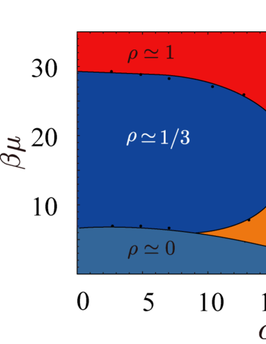
Figure 13: Phase diagram of t-J_z model in the grand-canonical ensemble. There are five phases and they are separated by first-order phase transition lines. SS stands for supersolid. $c_{Jz}=10.0$.

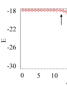
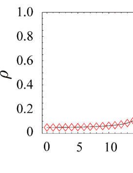
Figure 14: Behavior of internal energy and hole density at phase boundaries of supersolid indicating phase transitions at $c_{t}\simeq 12.0$ and $c_{t}\simeq 20.0$, where $\beta\mu=5$. Arrows indicate the location of phase transitions.

The obtained phase diagram by the MC simulations is shown in Fig.13. Phase transition from the pure-spin state to the supersolid is of second order and the others are of first order. The locations of the phase boundary are determined by the measurement of $E$ and $C$. As we expected, there is a parameter region in which the supersolid forms. The behavior of the internal energy and hole density are shown in Fig.14 at the phase boundary of the supersolid. Correlation functions to be used for identify the supersolid are explicitly shown in Fig.15. The correlation of the $z$-component of spin indicates there exists solid order, and the particle correlation shows the existence of a small but finite long-range order, i.e., superfluidity.

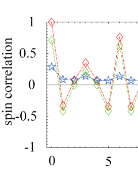
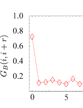
Figure 15: Spin and particle correlation functions in supersolid. $c_{t}=17$ and $\beta\mu=5$.

4 Conclusion and discussion

In this paper we studied phase diagram of the bosonic t-J model in the stacked triangular lattice. The model has a rich phase structure and we expect that some of them are observed by experiment on systems of two-component cold atomic gas and strongly correlated electron systems.

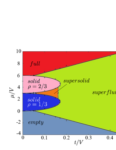
Figure 16: Phase diagram of the hard-core boson system in the stacked triangular lattice.[4] In this figure, $\rho$ denotes the particle density. $V$ and $t$ are parameters of the repulsion and hopping, and we set $\beta V=50$ (low-$T$ region). There exists a supersolid state between two solid states.

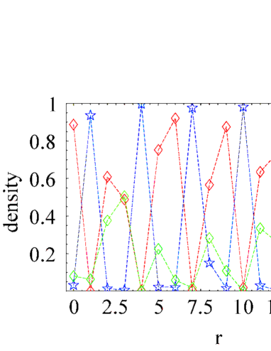
Figure 17: Density profiles of $a$, $b$-atoms and hole in the supersolid. $c_{Jz}=10.0,\ c_{t}=17.0$ and $\beta\mu=5.0$.

It is interesting to compare the obtained phase diagrams with that of the hard-core boson system in Ref.[4], which is shown in Fig.16. In the model Hamiltonian, $V$ represents the nearest-neighbor repulsive interaction and $t$ is the hopping parameter. There are two solid states with the particle density $\sim 1/3$ and $2/3$, and a supersolid state between them. The phase diagram in Fig.16 respects the particle-hole symmetry of the model, whereas in the t-J model such a symmetry does not exist. In the t-J_xy model studied in the paper, the supersolid does not form in similar parameter region and the phase separation takes place there instead, whereas in the t-J_z model the supersolid appears as in the hard-core boson system. For t-J_xy model with $t>0$, the reason why the phase-separated state dominates was explained in Sec.3.2. The state shown in Fig.6 corresponds to the state with the particle density $=2/3$ in the hard-core boson system. In the t-J model, the state with particle density $=1/3$ generally does not have spin long-range order nor solid (density-wave) order because of the low particle density and the non-existence of the particle-hole symmetry. Structure of the supersolid in the t-J_z model is slightly different from that observed in the hard-core boson system. The particle density there is larger than $2/3$, and one kind of atom, e.g., $b$-atoms occupy $B$-sublattice and $a$-atoms and holes form a superposed state in $A$ and $C$-sublattices. See Fig.17. Therefore for appearance of the supersolid in the t-J_z model, spin degrees of freedom plays an essential role. On the other hand in the hard-core bosons on the triangular lattice, the supersolid can be interpreted as a superfluid of excess bosons (or holes) via a relay-type movement.

It is interesting and useful to discuss the relation between the bosonic t-J model studied in this paper and the fermionic t-J model on the triangular lattice whose phase diagram was studied by high-temperature expansion in Ref.[11]. For the Hubbard model on the square lattice, very recent study by the numerical link-cluster expansion shows that the Fermi-Hubbard and Bose-Hubbard have a very similar physical properties for large on-site repulsions[12]. On the other hand in Ref.[11], the authors studied the fermionic t-J model on the triangular lattice and concluded that the RVB state appears by hole doping into the state with the three-sublattice spin symmetry for $t>0$ and $\rho=0.2-0.6$. By the high-temperature expansion, they found that the entropy decreases considerably at low temperature and peak of the spin susceptibility moves to the high-temperature region. These results indicate that the hole doping releases the frustration and enhances AF correlation though AF long-range order is not observed. In their discussion on the realized state, it was assumed that the low-temperature state is homogeneous and metallic. If this assumption is correct, the conclusion that the RVB forms at low-temperature seems plausible and acceptable. However the results obtained in this paper clearly offers another interpretation of their calculations, i.e., the state shown in Fig.6 has obviously has lower entropy and stable AF correlation compared to the 120^o spin state at $\rho=0$. Holes are localized there and the state is inhomogeneous contrary to the assumption in Ref[11]. We expect that a similar state to that in Fig.6 is realized in the fermionic model, though the superfluid in Fig.3 corresponds to a metallic phase of mobile holes in the fermionic t-J model. On the other hand for $t<0$, it was found in Ref.[11] that the entropy remains large until very low temperature and therefore the hole doping does not release the spin frustration at $\rho=0$. This result is also consistent with the results shown, e.g., in Fig.12.

In the above discussion on the bosonic and fermionic t-J models on the triangular lattice, we directly compared the obtained results for the models, and concluded that there is a close resemblance between two models. It is important and interesting to show the relationship between two model by an analytical method. To this end, discussion using the Chern-Simons gauge theory in Ref.[10] is useful. In the slave-particle representation (2), the Hamiltonian (1) is expressed as

$$H_{\rm tJ} = -t\sum_{\langle i,j\rangle,\sigma}(\varphi^{\dagger}_{\sigma i}\phi_{i}\phi^{\dagger}_{j}\varphi_{\sigma j}+\mbox{h.c.})$$ (7)

$$+J\sum_{\langle i,j\rangle,\sigma,\sigma^{\prime}}(\epsilon_{\sigma\bar{\sigma}}\varphi^{\dagger}_{\bar{\sigma}i}\varphi^{\dagger}_{\sigma j}\epsilon_{\sigma^{\prime}\bar{\sigma}^{\prime}}\varphi_{\sigma^{\prime}j}\varphi_{\bar{\sigma}^{\prime}i}+\mbox{h.c.})P_{i}P_{j},$$

$$P_{i}=1-\phi^{\dagger}_{i}\phi_{i},$$

where $\bar{\sigma}=2(1)$ for $\sigma=1(2)$, $\epsilon_{12}=-\epsilon_{21}=1,\ \epsilon_{11}=\epsilon_{22}=0$, and we have set $J_{z}=J$ for simplicity. On the other hand, the Hamiltonian of the fermionic t-J model in two spatial dimensions is given as follows by using the Chern-Simons gauge fields $A^{h}_{ij}$ and $A^{s}_{ij}$ defined on the link $(i,j)$[10, 22],

$$H^{\rm F}_{\rm tJ} = -t\sum_{\langle i,j\rangle,\sigma}(e^{iA^{s}_{ij}}e^{-i\sigma A^{h}_{ij}}\varphi^{\dagger}_{\sigma i}\phi_{i}\phi^{\dagger}_{j}\varphi_{\sigma j}+\mbox{h.c.})$$ (8)

$$+J\sum_{\langle i,j\rangle,\sigma,\sigma^{\prime}}(e^{-i\sigma A^{h}_{ij}}\epsilon_{\sigma\bar{\sigma}}\varphi^{\dagger}_{\bar{\sigma}i}\varphi^{\dagger}_{\sigma j}e^{i\sigma^{\prime}A^{h}_{ij}}\epsilon_{\sigma^{\prime}\bar{\sigma}^{\prime}}\varphi_{\sigma^{\prime}j}\varphi_{\bar{\sigma^{\prime}}i}+\mbox{h.c.})P_{i}P_{j},$$

where $\sigma A\equiv A\ (-A)$ for $\sigma=1\ (2)$, and

$$\sum_{(i,j)\in{\cal C}}A^{s}_{ij}=\pi\sum_{(i,j)\ {\rm inside}\ {\cal C}}(\varphi^{\dagger}_{1}\varphi_{1}-\varphi^{\dagger}_{2}\varphi_{2}),\;\mbox{mod}\ 2\pi,$$

$$\sum_{(i,j)\in{\cal C}}A^{h}_{ij}=\pi\sum_{(i,j)\ {\rm inside}\ {\cal C}}(\phi^{\dagger}\phi-\rho),\;\mbox{mod}\ 2\pi,$$ (9)

where ${\cal C}$ is a closed loop and $A_{ij}=-A_{ji}$ is understood in the above summations in (9). In the homogeneous state, we can replace the RHS’s of Eq.(9) by their mean values for investigating the ground-state phase diagram. In the case of the coplanar spin configuration as we considered in this paper, effects of $A^{s}_{ij}$ is small because $\langle(\varphi^{\dagger}_{1}\varphi_{1}-\varphi^{\dagger}_{2}\varphi_{2})\rangle=0$. Similarly for a homogeneous hole distribution, the Chern-Simons gauge field $A^{h}_{ij}$ can be set $A^{h}_{ij}=0$ in the mean-field level. Therefore for a homogeneous state, phase diagrams of $H_{\rm tJ}$ and $H^{\rm F}_{\rm tJ}$ are closely related with each other, though dispersion relation of excitations in the two systems are different by the local constraints Eq.(9), i.e., in the system $H^{\rm F}_{\rm tJ}$, hopping of bosonic spinon and holon accompanies the Chern-Simons flux[23]. Anyway, more detailed study on the relation between the two models by using the Chern-Simons gauge theory is interesting and useful[24].

This work was partially supported by Grant-in-Aid for Scientific Research from Japan Society for the Promotion of Science under Grant No23540301.

References

- [1] E. Kim and M.H.W. Chan, Nature (London) 427, 225 (2004); Science 305, 1941 (2004).
- [2] For review, see, e.g., I. Bloch, J. Dalibard, and W. Zwerger, Rev. Mod. Phys.80, 885 (2008); M. Lewenstein, A. Sanpera, V. Ahufinger, B. Damski, A. S. De, and U. Sen, Adv. Phy. 56, 243 (2008).
- [3] S. Wessel and M. Troyer, Phys. Rev. Lett. 95, 127205 (2005).
- [4] H. Ozawa and I. Ichinose, Phys. Rev. A 86, 015601 (2012).
- [5] A.F. Andreev and I.M. Lifshitz, Sov. Phys. JETP29, 1107 (1969); G. Chester, Phys.Rev. A 2, 256(1970).
- [6] Y. C. Chen, R. G. Melko, S. Wessel, and Y. J. Kao, Phys. Rev. B 77, 014524 (2008); L. Dang, M. Boninsegni, and L. Pollet, Phys. Rev. B 78, 132512 (2008).
- [7] M. Boninsegni, Phys. Rev. Lett. 87, 087201 (2001); Phys. Rev. B 65, 134403 (2002).
-
[8]
For the Mott-insulator region, see
A. B. Kuklov and
B. V. Svistunov, Phys. Rev. Lett. 90, 100401 (2003);
L. M. Duan, E. Demler, and M. D. Lukin, Phys. Rev. Lett. 91, 090402 (2003). - [9] Y. Nakano, T. Ishima, N. Kobayashi, T. Yamamoto, I. Ichinose, and T. Matsui, Phys. Rev. A 85, 023617(2012).
-
[10]
Z. Y. Weng, D. N. Sheng, Y. C. Chen, and C. S. Ting,
Phys. Rev. B 55, 3894 (1997);
P. Ye, C.S. Tian, X.L. Qi, and Z.Y. Weng, Phys. Rev. Lett. 106, 147002 (2011). - [11] T. Koretsune and M. Ogata, Phys. Rev. Lett. 89, 116401 (2002).
- [12] E. Khatami and M. Rigol, Phys. Rev. A 86, 023633 (2012).
- [13] Y. Nakano, T. Ishima, N. Kobayashi, K. Sakakibara, I. Ichinose, and T. Matsui, Phys. Rev. B 83, 235116 (2011); A. Shimizu, K. Aoki, K. Sakakibara, I. Ichinose, and T. Matsui, Phys. Rev. B 83, 064502 (2011).
- [14] K. Sawamura, T. Hiramatsu, K. Ozaki, I. Ichinose, and T. Matsui, Phys. Rev. B 77, 224404(2008).
- [15] K. Nakane, T. Kamijo, and I. Ichinose, Phys. Rev. B 83, 054414 (2011).
-
[16]
S. D. Huber, B. Theiler, E. Altman, and G. Blatter,
Phys. Rev. Lett. 100, 050404 (2008);
L. Pollet and N. Prokof’ev, Phys. Rev. Lett. 109, 010401 (2012). -
[17]
N.Metropolis, A.W.Rosenbluth, M.N.Rosenbluth,
A.M.Teller, and E.Teller,
J. Chem. Phys.21, 1087(1953);
J. M. Thijssen, “Computational Physics”, (Cambridge University Press, 1999). - [18] F. Wang, F. Pollmann, and A. Vishwanath, Phys. Rev. Lett. 102, 017203 (2009); D. Heidarian and K. Damle, Phys. Rev. Lett. 95, 127206 (2005); R. G. Melko, et al., Phys. Rev. Lett. 95, 127207 (2005).
-
[19]
Y. Ishibashi, M. Iwata, Jpn. J. App. Phys. 37, L985 (2005);
H. Fu and R. E. Cohen, Nature (London) 403, 281 (2000). - [20] P. W. Anderson, Mater. Res. Bull. 8, 153 (1973); Science 235, 1196 (1987).
-
[21]
S. Tung, V. Schweikhard, and E. A. Cornell,
Phys. Rev. Lett. 97, 240402 (2006);
R. A. Williams, S. Al-Assan, C. J. Foot, Phys. Rev. Lett. 104, 050404 (2010). - [22] I. Ichinose and T. Matsui, Nucl. Phys. B 468 [FS], 487 (1996); Nucl. Phys. B 483 [FS], 681 (1997).
- [23] S. C. Zhang, Int. J. Mod. Phys. B 6, 25 (1992); For multi-component case, I. Ichinose and A. Sekiguchi, Nucl. Phys. B 493 [FS], 683 (1997).
- [24] B.-L. Chen and S.-P. Kou, Mod. Phys. Lett. B25 (2011)813.