Novel Aharonov-Bohm-like effect: Detectability of the vector potential in a solenoidal configuration with a ferromagnetic core covered by superconducting lead, and surrounded by a thin cylindrical shell of aluminum

Abstract

The flux as measured by the Josephson effect in a SQUID-like configuration with a ferromagnetic core inserted into its center, is shown to be sensitive to the vector potential arising from the central ferromagnetic core, even when the core is covered with a superconducting material that prevents any magnetic field lines from ever reaching the perimeter of the SQUID-like configuration. This leads to a macroscopic, Aharonov-Bohm-like effect that is observable in an asymmetric hysteresis loop in the response of the SQUID-like configuration to an externally applied magnetic field.

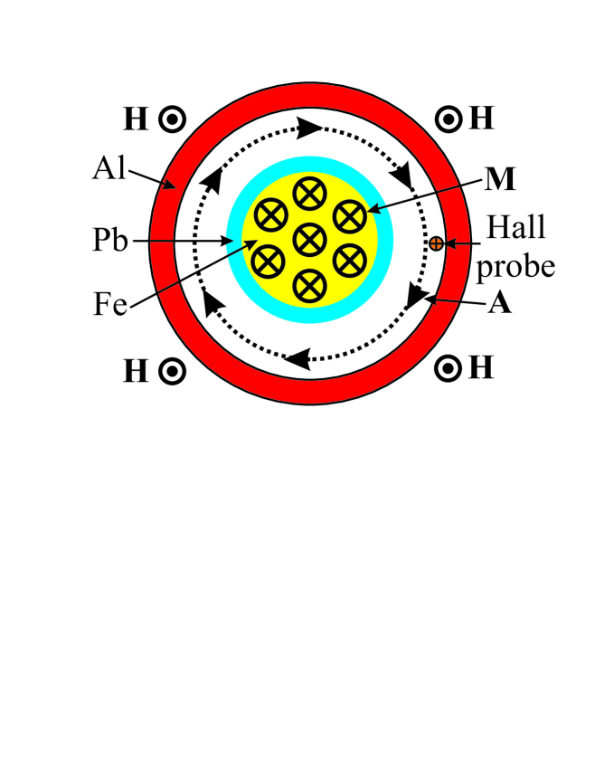
Figure 1: A solenoidal configuration consists of an infinitely long ferromagnetic core (yellow) coated by a thick layer of lead (blue), at the center of a thin cylindrical shell of aluminum (red). $\bf{H}$ is an externally applied magnetic field, $\bf{M}$ the magnetization of the ferromagnetic core, and $\bf{A}$ the vector potential. As the temperature is steadily lowered, the lead (blue) coating first becomes superconducting, and totally confines the ferromagnetic flux to the interior of the core via the Meissner effect, so that the aluminum ring detects no $\bf{B}$ field arising from the core, but detects the $\bf{A}$ field. As the temperature is further lowered, the aluminum (red) ring becomes superconducting, and acquires a persistent current which measures the core’s $\bf{A}$ field via a SQUID-like flux trapping effect.

In our ongoing experiments [1], we are using a ferromagnetic torus coated with a superconductor (lead) [2], which is topologically linked with another superconducing (SC) ring made out of a different material (aluminum), which has a lower critical temperature. However, to understand this experiment more easily, let us first consider the simpler cylindrically-symmetric configuration of Figure 1, which depicts a straight, infinitely long solenoidal configuration consisting of a cylindrical ferromagnetic core (yellow) possessing a permanent magnetization $\bf{M}$, which is covered with a thick coating of SC lead (blue), in order to prevent, due to the Meissner effect, any stray magnetic flux lines from escaping from the core. This core in turn is placed at the center of a thin cylindrical shell of SC aluminum (red), which has a lower critical temperature than that of SC lead (blue).

Let us further assume that the temperature has been cooled to near absolute zero, and that we are slowly applying a uniform magnetic field $\bf{H}$ onto the entire assembly starting from zero field. The magnetostatic flux filling the ferromagnetic core due to its permanent magnetization will give rise to a static contribution to the circular lines of the vector potential $\bf{A}$, as illustrated by the dashed circle in Figure 1. However, note that due to the Meissner effect arising from the thick lead coating, the magnetostatic field $\bf{B}$ arising from the ferromagnetic core vanishes in the spatial region in which the cylindrical shell of aluminum material resides, so that the electrons in this shell never experience any classical forces. This is true both above and below the critical temperature of the aluminum shell. Nevertheless, like in the Aharonov-Bohm effect, there exists a nonlocal quantum influence of the electrons within the ferromagnetic core upon the electrons within the superconducting shell, since persistent currents within the core can induce persistent currents within the shell that are proportional to the size of the vector potential arising from the ferromagnetic core.

The probability current density in quantum mechanics for a single neutral particle of mass $m$ moving through the vacuum is given by

$${\bf j} = \frac{\hbar}{2mi}\left(\psi^{\ast}{\bf\nabla}\psi-\psi{\bf\nabla}\psi^{\ast}\right)$$ (1)

$$= \frac{1}{2m}\left(\psi^{\ast}\left(\frac{\hbar}{i}{\bf\nabla}\right)\psi-\psi\left(\frac{\hbar}{i}{\bf\nabla}\right)\psi^{\ast}\right)$$

$$= \frac{1}{2m}\left(\psi^{\ast}{\bf p}_{{\rm op}}\psi\right)+{\rm c.c.}$$

where $\psi=\psi\left({\bf r},t\right)$ is the wavefunction evaluated at the spacetime point $\left({\bf r},t\right)$, and where the momentum operator in the configuration space representation is

$${\bf p}_{{\rm op}}=\frac{\hbar}{i}{\bf\nabla}$$ (2)

From the time-dependent Schrodinger equation, the continuity equation

$${\bf\nabla\cdot j}+\frac{\partial\rho}{\partial t}$$ (3)

follows, in which

$$\rho=\psi^{\ast}\psi=\psi^{\ast}\left({\bf r},t\right)\psi\left({\bf r},t\right)$$ (4)

is the probability density for finding the particle located at $\left({\bf r},t\right)$ upon measurement. The continuity equation (3) means that probability is conserved.

Let us generalize the above expression (1) for the probability current density ${\bf j}\left({\bf r},t\right)$ to that of a particle with charge $q$ moving through the vacuum in the presence of a vector potential ${\bf A}\left({\bf r},t\right)$, by applying the minimal coupling rule [1]

$${\bf p}_{{\rm op}}\rightarrow{\bf p}_{{\rm op}}-q{\bf A}$$ (5)

to (1). Then one finds that for the particle with charge $q$

$${\bf j}=\frac{1}{2m}\left(\psi^{\ast}\left(\frac{\hbar}{i}{\bf\nabla}-q{\bf A}\right)\psi\right)+{\rm c.c.}$$ (6)

This expression for the probability current density ${\bf j}\left({\bf r},t\right)$ for the charge $q$ moving through the vacuum generalizes to an expression for the supercurrent density ${\bf J}_{s}\left({\bf r},t\right)$ for Cooper pairs moving through a SC, which can be obtained from the complex order parameter $\Psi\left({\bf r},t\right)$ of the Ginzburg-Landau theory as follows:

$${\bf J}_{s}=\frac{1}{2m}\left(\Psi^{\ast}\left(\frac{\hbar}{i}{\bf\nabla}-q{\bf A}\right)\Psi\right)+{\rm c.c.}$$ (7)

where $q=2e$ is the charge and $m=2m_{e}$ is the mass of the Cooper pair.

Next, let us express the complex order parameter $\Psi$ in polar form as follows:

$$\Psi=\sqrt{\rho}e^{i\phi}$$ (8)

where

$$\rho=\Psi^{\ast}\Psi$$ (9)

is the probability density of Cooper pairs, and where $\phi$ is the local phase of the Cooper pair’s “macroscopic wavefunction” $\Psi$.

Since the local positive charge density of the background ionic lattice must be exactly locally compensated by the local negative charge density of the Cooper pairs in order to preserve the overall charge neutrality of the SC material (which must be true under all conceivable experimental circumstances), we require that

$$\left|\rho\right|=\left|\rho_{{\rm ioniclattice}}\right|={\rm constant}$$ (10)

independent of space and time. Therefore, to an extremely good approximation, the density of Cooper pairs

$$\rho\left({\bf r},t\right)=\rho_{0}$$ (11)

is independent of $\left({\bf r},t\right)$; only their phase $\phi=\phi\left({\bf r},t\right)$ is allowed to vary with space and time inside the SC. Hence the polar decomposition (8) becomes

$$\Psi\left({\bf r},t\right)=\sqrt{\rho_{0}}e^{i\phi\left({\bf r},t\right)}$$ (12)

Therefore the supercurrent density (7) becomes

$${\bf J}_{s} = \frac{1}{2m}\left(\sqrt{\rho_{0}}e^{-i\phi}\left(\frac{\hbar}{i}\left(i{\bf\nabla}\phi\right)-q{\bf A}\right)\sqrt{\rho_{0}}e^{i\phi}\right)+{\rm c.c.}$$ (13)

$$= \frac{\rho_{0}}{2m}\left(\frac{\hbar}{i}\left(i{\bf\nabla}\phi\right)-q{\bf A}\right)+{\rm c.c.}$$

$$= \frac{\rho_{0}}{m}\left(\hbar{\bf\nabla}\phi-q{\bf A}\right)=\rho_{0}{\bf v}_{s}$$

where ${\bf v}_{s}$ is the superfluid velocity of the Cooper pairs. Hence the supercurrent density becomes

$${\bf J}_{s}=\rho_{0}{\bf v}_{s}=\frac{\rho_{0}}{m}\left(\hbar{\bf\nabla}\phi-q{\bf A}\right)$$ (14)

and therefore

$$m{\bf v}_{s}=\hbar{\bf\nabla}\phi-q{\bf A}$$ (15)

where $m{\bf v}_{s}$ is the kinetic momentum, $\hbar{\bf\nabla}\phi$ is the canonical momentum, and $q{\bf A}$ is the electromagnetic momentum of the Cooper pairs.

The concept of fluxoid quantization follows from (15), by integration over a circular path inside the material of the red cylindrical shell of Figure 1 as follows:

$$m\oint{\bf v}_{s}\cdot d{\bf l}=\hbar\oint{\bf\nabla}\phi\cdot d{\bf l}-q\oint{\bf A}\cdot d{\bf l}$$ (16)

Due to the single-valuedness of complex order parameter $\Psi$, it follows that

$$\oint{\bf\nabla}\phi\cdot d{\bf l}=2\pi n,{\rm}(n=0,\pm 1,\pm 2,...)$$ (17)

and therefore that

$$q\oint{\bf A}\cdot d{\bf l+}m\oint{\bf v}_{s}\cdot d{\bf l}=2\pi n\hbar=nh,{\rm}(n=0,\pm 1,\pm 2,...)$$ (18)

Let us define the fluxoid as follows:

$$\Phi_{{\rm fluxoid}}\equiv\oint\left({\bf A+}\frac{m}{q}{\bf v}_{s}\right)\cdot d{\bf l}=\Phi+\frac{m}{q}\kappa$$ (19)

where

$$\Phi=\oint{\bf A}\cdot d{\bf l}$$ (20)

is the flux, and where

$$\kappa=\oint{\bf v}_{s}\cdot d{\bf l}$$ (21)

is the circulation of the superfluid, which can become important when the cylindrical shell becomes thin compared to the penetration depth of the SC (here, aluminum), as happens when the applied magnetic $H$ field approaches the critical field $H_{{\rm c}}$. It follows from (18) that the fluxoid obeys the following quantization condition:

$$\Phi_{{\rm fluxoid}}=n\frac{h}{2e}=n\Phi_{0},{\rm}(n=0,\pm 1,\pm 2,...)$$ (22)

where

$$\Phi_{0}=\frac{h}{2e}=2.07\times 10^{-15}{\rm webers}$$ (23)

is the quantum of flux. However, if the cylindrical shell is thick compared to the penetration depth, then the circulation $\kappa$ for the superfluid deep inside the red ring of Figure 1 becomes negligible, and fluxoid quantization reduces to the usual flux quantization condition, where

$$\Phi_{{\rm flux}}\equiv\oint{\bf A}\cdot d{\bf l}=\Phi_{n}=n\frac{h}{2e}=n\Phi_{0},{\rm}(n=0,\pm 1,\pm 2,...)$$ (24)

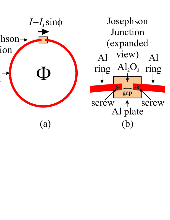
Figure 2: (a) SQUID-like model for the production of a persistent supercurrent $I$ within a SC ring (in red) by a total enclosed flux $\Phi$, when the ring is interrupted by a Josephson junction possessing a critical current $I_{{\rm J}}$. The self-inductance $L$ of the ring will lead to the onset of a remnant field and hysteresis. (b) Expanded view of the Josephson junction. An aluminum plate (pink) with an oxidized sapphire surface (Al₂O₃), when screwed tightly onto the gapped aluminum ring (i.e., in the form of a flat gasket with a gap in it), makes the ring into a closed SC circuit containing a single, effective Josephson junction in it.

Figure 2(a) depicts a SQUID-like model for the nonlinearity that occurs within the red cylindrical shell in Figure 1 as the externally applied magnetic field passes through the effective critical field of the SC material (i.e., the aluminum ring plus an effective Josephson junction). This nonlinearity is essential for a breakdown of the superposition principle for electromagnetic fields in a vacuum, which permits the detection of the vector potential arising from the ferromagnetic core of the configuration shown in Figure 1. Note that we have replaced the red cylindrical shell of Figure 1 by a red ring in the form of a thin, flat circular gasket which has a gap in it, as shown in Figure 2(b), so as to be able to incorporate the Meissner-shielded ferromagnetic core into its center during the assembly process.

One justification for using this SQUID-like model [3][4][5] goes as follows: The ring gasket of aluminum in Figure 2(a) must have a large enough gap cut into it in order to enable the ferromagnetic torus to slip by the gap and enter into the center of the SC ring, in order to realize the configuration of Figure 1. But in order to form a complete SC circuit, the gap in the aluminum gasket will be filled in by pressing onto the top of the gap an overlapping rectangular aluminum plate (shown in pink in Figure 2(b)), which covers the gap. Thus a topological “link” can be formed between a “ring” and a “torus”[1], with the same topology as that in Figure 1.

Two small screws, which are drilled into the two overlap areas between the rectangular plate and the gapped gasket, will be used to press tightly the flat, rectangular aluminum plate onto the gapped region of the flat aluminum gasket, and thus to complete a SC circuit. However, since the aluminum material of the ring and of the plate will naturally form an oxide (Al₂O₃) layer on its surfaces, two oxide-layer Josephson junctions will naturally be formed at the two overlap areas between the plate and the ring, after the rectangular plate has been pressed tightly onto the gapped ring by means of these two small screws. The resulting two in-series, oxide-barrier Josephson junctions of Figure 2(b) can be thought of as being a single, effective Josephson junction interrupting the ring. This effective Josephson junction will obey the following sinusoidal relationship [3]:

$$I=I_{{\rm J}}\sin\phi$$ (25)

where $I$ is the supercurrent flowing through the junction, $I_{{\rm J}}$ is the effective Josephson critical current, and $\phi$ is the phase difference across the junction, which, for configuration shown in Figure 2(a), is given by the Aharonov-Bohm phase

$$\phi=\frac{q}{\hbar}\oint{\bf A}\cdot d{\bf l}=2\pi\frac{\Phi}{\Phi_{0}}\propto\Phi$$ (26)

where $\Phi$ is the total flux enclosed by the ring and

$$\Phi_{0}=\frac{h}{2e}$$ (27)

is the quantum of flux. Thus the phase shift $\phi$ is directly proportional to the total flux $\Phi$ enclosed by the ring. Note that this implies that there exists a nonlinear relationship exists between the supercurrent $I$ and the total flux $\Phi$, on account of the sinusoidal nature of (25).

Hysteresis in the ring can arise from the self-inductance of the ring as follows: The total flux enclosed by the ring will be sum of two terms

$$\Phi=\Phi_{H}+\Phi_{I}$$ (28)

where $\Phi_{H}$ is the flux imposed onto the ring from a pair of Helmholtz coils, i.e., by an externally applied $H$ field, and $\Phi_{I}$ is the flux generated by the self-inductance of the ring due to the supercurrent $I$. For simplicity, we shall first consider the case where the width of the ring is less than the effective penetration depth, and where we are imposing an external field close to the effective critical field $H_{{\rm c}}$, so that the exterior, imposed flux can freely flow in or out from the interior of the ring near “criticality”.

Now the flux generated by the Josephson supercurrent $I$ via the inductance $L$ of the ring obeys the relationship

$$\Phi_{I}=LI$$ (29)

where $L$ is the self-inductance of the ring. Putting this together with (25), one obtains the transcendental equation

$$I=I_{{\rm J}}\sin\left\{\frac{2\pi}{\Phi_{0}}\left(\Phi_{H}+LI\right)\right\}$$ (30)

One can express this equation as two equations in two unknowns, $\Phi$ and $I$, as follows:

$$I = I_{{\rm J}}\sin\left(\frac{2\pi}{\Phi_{0}}\Phi\right)$$ (31)

$$\Phi = \Phi_{H}+LI$$ (32)

One can rewrite the second equation as the following linear equation for $I$ in terms of $\Phi$:

$$I=\frac{1}{L}\left(\Phi-\Phi_{H}\right)$$ (33)

which has the form of a straight-line relationship

$$I=a\Phi+b$$ (34)

where

$$a=\frac{1}{L}$$ (35)

and

$$b=-\frac{\Phi_{H}}{L}$$ (36)

are the slope and the intercept of the straight-line relationship (34), respectively.

A graphical method of solution to the transcendental equation expressed as the two equations (31) and (34) is illustrated in Figure 3.

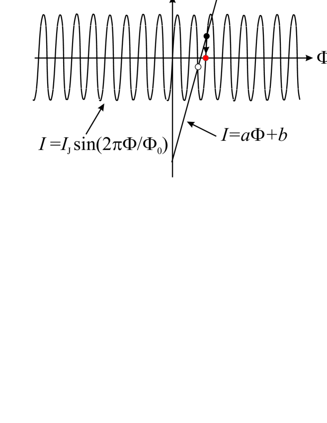
Figure 3: Graphical method (not to scale) for the solution of the transcendental equation (30), written as the two equations (37) and (38). The intercept at the black dot represents a stable solution, and that at the white dot an unstable solution. The red dot represents the nearest possible metastable flux-trapping state (i.e., a persistent-current state), which possesses an integer multiple of flux quanta $\Phi_{0}$ trapped within the ring, i.e., a nonzero remnant magnetization when $H\rightarrow 0$. Since $\Phi_{0}$ is a very small quantity, the sinusoidal oscillations of $I$ are very rapid, and the flux-trapping states are highly metastable.

The intercepts (the black and the white dots) between the two graphs

$$I = I_{{\rm J}}\sin\left(\frac{2\pi}{\Phi_{0}}\Phi\right){\rm and}$$ (37)

$$I = a\Phi+b$$ (38)

represent the graphical solutions to the transcendental equation. The white dot presents an unstable solution (one with an “anti-Lenz” Faraday-like law). The black dot solution will eventually settle down to the nearest possible metastable, persistent current solution, which is represented by the red-dot solution, after the applied magnetic field is reduced to zero, and a quantized number of flux lines corresponding to the red-dot solution, has been trapped inside the ring. This happens when one reduces the external field to values well below the effective critical field $H_{{\rm c}}$, where the effective penetration depth becomes much smaller than the width of the red ring. As one further reduces the applied field until it reaches zero, i.e., as $H\rightarrow 0$, the remnant field as measured by the Hall probe in Figure 1 will approximately be the trapped flux corresponding to the red-dot solution, divided by the area of the ring. (However, the above analysis is for a one-dimensional ring, and needs to be generalized to a three-dimensional ring in order to confirm the above conclusions. See Appendix A.)

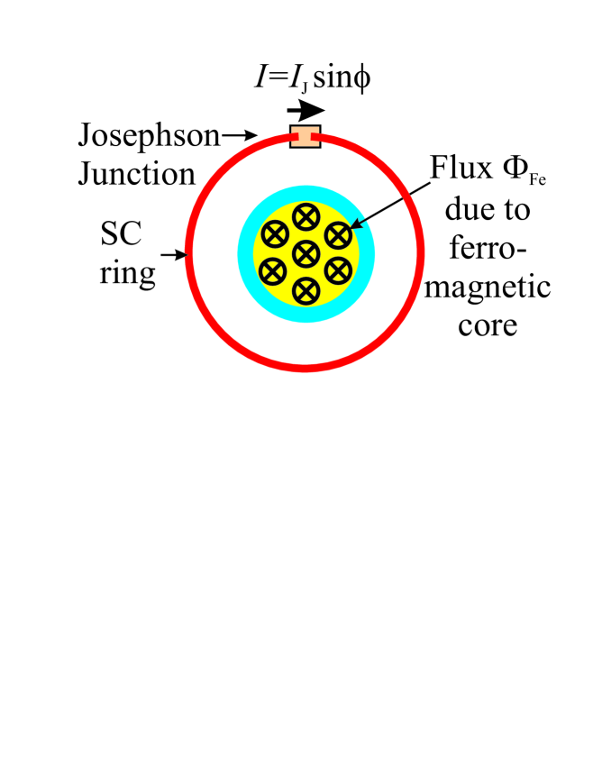
Figure 4: SQUID-like model of Figure 2(a) after the insertion of a ferromagnetic core (yellow) overcoated by a thick SC coating of lead (blue) into its center (not to scale). The flux from the ferromagnetic core contributes to the flux seen by the Josephson junction (pink), even though only the vector potential, but not the ferromagnetic field from the core, reaches the SC aluminum ring (red).

The way to extend the above ideas to the configuration in Figure 1 where there is a ferromagnetic core thickly overcoated by a strong SC such as lead or lead-tin solder, is obvious from an inspection of Figure 4. The above analysis is changed by adding the flux $\Phi_{{\rm Fe}}$ arising from the ferromagnetic core to the total flux seen by the Josephson junction, i.e.,

$$\Phi=\Phi_{H}+\Phi_{I}+\Phi_{{\rm Fe}}$$ (39)

This has the effect of adding a DC bias to the flux in the graphical solution of Figure 3 by an amount $\Phi_{{\rm Fe}}$, thus either increasing or decreasing, depending on the sign of $\Phi_{{\rm Fe}}$, the remnant magnetic field as measured by the Hall probe in Figure 1. This analysis also extends to the case of a ferromagnetic torus thickly coated with a strong SC (e.g., lead) linked with a ring composed of a weak SC (e.g., aluminum or tin), as pictured in the first Figure of [1].

1 Appendix A: Case of a wide aluminum ring.

An external magnetic field $H$ imposed upon the wide aluminum ring in Figure 2 will lead to an inner current $I_{{\rm inner}}$ flowing along the inner perimeter of the ring within a penetration depth, and an outer current $I_{{\rm outer}}$ flowing along the outer perimeter of the ring within a penetration depth. These two currents will join together at the effective Josephson junction to satisfy the Josephson sinusoidal relationship

$$I=I_{{\rm inner}}+I_{{\rm outer}}=I_{{\rm J}}\sin\phi$$ (40)

The metastable solutions corresponding to flux quantization in integer multiples of the flux quantum, such as the case of the red-dot solution in Figure 3, corresponds to solutions with the discrete Aharonov-Bohm phase values

$$\phi_{n}=2\pi n,{\rm}(n=0,\pm 1,\pm 2,...)$$ (41)

i.e., the zero-crossings of the sine function (40), or to the quantized flux values

$$\Phi_{n}=n\frac{h}{2e},{\rm}(n=0,\pm 1,\pm 2,...)$$ (42)

The free energy of the system will have extremely deep, local minima at these quantized values of the flux, which correspond to the extremely metastable solutions for the wide ring at the effective critical values of the applied magnetic field (i.e., at “criticality”) where

$$I_{n}=\left.I_{{\rm inner}}\right|_{n}+\left.I_{{\rm outer}}\right|_{n}=I_{{\rm J}}\sin\phi_{n}=0$$ (43)

In other words, at “criticality”, the inner and outer currents will satisfy the relationship

$$\left.I_{{\rm inner}}\right|_{n}=-\left.I_{{\rm outer}}\right|_{n}$$ (44)

However, as the externally applied magnetic field $H$ is subsequently reduced to zero, the inner current must remain constant, since the interior flux must remain quantized, whilst the outer current will be reduced to zero along with the vanishing exterior $H$ field, i.e.,

$$\left.I_{{\rm inner}}\right|_{n}\rightarrow\frac{\Phi_{n}}{L}{\rm}$$ (45)

as $H\rightarrow 0$, but

$$\left.I_{{\rm outer}}\right|_{n}\rightarrow 0$$ (46)

as $H\rightarrow 0$. Thus there will result a “remnant” field contained within the inner perimeter of the ring, which will approach the value

$$B_{{\rm remnant}}\rightarrow\frac{\Phi_{n}}{\mathcal{A}}$$ (47)

as $H\rightarrow 0$, where $\mathcal{A}$ is the inner area of ring (excluding the cross-sectional area of the torus), which can be measured by the Hall probe (orange) in Figure 1. This leads to the possibility of an observation of the “asymmetric hysteresis” phenomenon in the linked torus-ring system, as described in [1].

In summary, the flux measured in the Josephson effect in a SQUID-like configuration with a ferromagnetic core is the total flux enclosed by this kind of SQUID, including the flux from the ferromagnetic core, as illustrated in Figure 4. It is this that leads to the macroscopic, Aharonov-Bohm-like effect described here.

References

- [1] R.Y. Chiao, “Hysteretic method for measuring the flux trapped within the core of a superconducting lead-coated ferromagnetic torus by a linked superconducting tin ring, in a novel Aharonov-Bohm-like effect based on the Feynman path-integral principle”, arXiv:1205.6029.
- [2] A. Tonomura, N. Osakabe,T. Matsuda, T. Kawasaki, J. Endo, S. Yano, and H. Yamada, “Evidence for Aharonov-Bohm effect with magnetic field completely shielded from electron wave,” Phys. Rev. Lett. 56, 792 (1986); A. Tonomura, “New results on the Aharonov-Bohm effect with electron interferometry,” Physica B 151, 206 (1988).
-
[3]
Another justification for the Josephson sinusoidal
relationship (25) for the thin red SC
rings in Figures 1 and 2, is a more general one based solely on the gauge
symmetry considerations given by F. Bloch, which starts from the fact that
the free energy of the thin ring (i.e., thin compared to the penetration
depth), like that of any homogeneous many-electron system with an
off-diagonal long-range order, must be a periodic function of the flux
enclosed by the ring with a period of quantum of flux given by (27), i.e.,
This follows from the principle of local gauge invariance and the Aharonov-Bohm effect. Due to the inversion symmetry of space, the free energy(48)
must be an even function of the flux . Since the free energy is related to the power delivered to the ring by(49)
the supercurrent induced in the ring is related to the free energy by(50)
Since is a periodic, even function of the flux , the supercurrent must a periodic, odd function of the flux , i.e.,(51)
A Fourier series expansion of any periodic function, such as (52), with an odd parity symmetry, such as (53), must have as its leading term (i.e., as the fundamental harmonic term)(52) (53)
with some unknown Fourier expansion coefficient , which must be determined by experiment. Bloch’s sinusoidal relationship (54) is another form of the Josephson relationship (25). See F. Bloch, “Off-diagonal long-range order and persistent currents in a hollow cylinder”, Phys. Rev. 137, A787 (1965); “Simple interpretation of the Josephson effect”, Phys. Rev. Lett. 21, 1241 (1968); “Josephson effect in a superconducting ring”, Phys. Rev. B2, 109 (1970).(54) - [4] A.H. Silver and J.E. Zimmerman, “Quantum states and transitions in weakly connected superconducting rings”, Phys. Rev. 157, 317 (1967).
- [5] J.D. Jackel, R.A. Buhrman, and W.W. Webb, “Direct measurement of current-phase relations in superconducting weak links”, Phys. Rev. B10, 2782 (1974).