Notes on planar semimodular lattices. VII.
Resections of planar semimodular lattices

Abstract.

A recent result of G. Czédli and E. T. Schmidt gives a construction of slim (planar) semimodular lattices from planar distributive lattices by adding elements, adding “forks”. We give a construction that accomplishes the same by deleting elements, by “resections”.

June 23, 2012.

1. Introduction

In this paper, we present a construction of slim (planar) semimodular lattices from planar distributive lattices by a series of resections. A resection starts with a cover-preserving $\mathsf{C}_{3}^{2}$ (the dark gray square of the three-element chain in Figure 2), and it deletes two elements to get an $\mathsf{N}_{7}$ (see Figure 3) from $\mathsf{C}_{3}^{2}$, and then deletes some more elements (all the black-filled ones), going up and down to the left and to the right, to preserve semimodularity; see Figure 2 for the result of the resection.

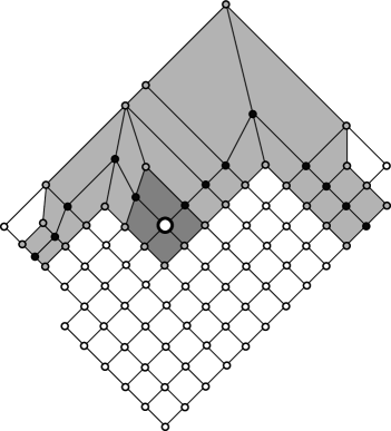
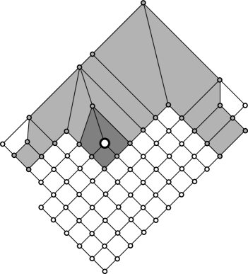
Figure 1. Resect this diagram at the element marked by the big circle by deleting the black-filled elements

Figure 2. to obtain this diagram

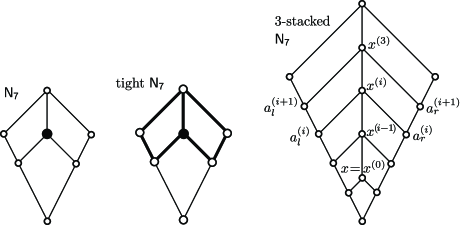
Figure 3. $\mathsf{N}_{7}$ and its variants

A lattice $L$ is slim if it is finite and $\operatorname{Ji}L$ contains no three-element antichain. Slim lattices are planar, so we will consider planar diagrams of slim semimodular lattices, slim semimodular diagrams, for short.

For the basic concepts and notation, we refer the reader to G. Grätzer [5] and G. Czédli and G. Grätzer [1].

Outline

Section 2 introduces resections. Section 3 states the main result. Section 4 recalls some known results on slim semimodular lattices and proves some facts on (the inverse of) resection schemes. Section 5 contains the proof of the main result.

2. The construction

Let $D$ be a slim semimodular diagram. Two prime intervals of $D$ are consecutive if they are opposite sides of a $4$-cell (see Section 4). As in G. Czédli and E. T. Schmidt [2], maximal sequences of consecutive prime intervals form a $\mathsf{C}_{2}$-trajectory. So a $\mathsf{C}_{2}$-trajectory is an equivalence class of the transitive reflexive closure of the “consecutive” relation.

Similarly, let $A$ and $B$ be two cover-preserving $\mathsf{C}_{3}$-chains of $D$. If they are opposite sides of a cover-preserving $\mathsf{C}_{3}\times\mathsf{C}_{2}$, then $A$ and $B$ are called consecutive. An equivalence class of the transitive reflexive closure of this “consecutive” relation is called a $\mathsf{C}_{3}$-trajectory.

We recall the basic properties of $\mathsf{C}_{2}$-trajectories from [2] and [4]; they also hold for $\mathsf{C}_{3}$-trajectories. For $i\in\{2,3\}$, a $\mathsf{C}_{i}$-trajectory goes from left to right (unless otherwise stated); they do not branch out. A $\mathsf{C}_{i}$-trajectory is of two types: an up-trajectory, which goes up (possibly, in zero steps) and a hat-trajectory, which goes up (possibly in zero steps), then turns to the lower right, and finally it goes down (possibly, in zero steps).

Note that the left and right ends of a $\mathsf{C}_{2}$-trajectory are on the boundary of $L$; this may fail for a $\mathsf{C}_{3}$-trajectory.

The elements of a $\mathsf{C}_{i}$-trajectory are the elements of the $\mathsf{C}_{i}$-chains forming it. Let $A$ be a cover-preserving $\mathsf{C}_{i}$-chain in $D$. By planarity, there is a unique $\mathsf{C}_{i}$-trajectory through $A$. The $\mathsf{C}_{i}$-chains of this trajectory to the left of $A$ and including $A$ form the left wing of $A$. The right wing of $A$ is defined analogously.

Next, let $B$ be a cover-preserving $\mathsf{C}_{3}^{2}=\mathsf{C}_{3}\times\mathsf{C}_{3}$ of the diagram $D$. Let $W_{l}$ be the left wing of the upper left boundary of $B$ and let $W_{r}$ be the right wing of the upper right boundary of $B$. Assume that $W_{l}$ and $W_{r}$ terminate on the boundary of $D$ (that is, the last $\mathsf{C}_{3}$-chains are on the boundary of $D$). In this case, the collection of elements of $S=B\cup W_{l}\cup W_{r}$ is called a $\mathsf{C}_{3}$-scheme of $D$, see Figure 2 for an example. The elements of $W_{l}$ and $W_{r}$ form the left wing and the right wing of this $\mathsf{C}_{3}$-scheme, respectively, while $B$ is the base. The middle element of $S$ is the anchor of the scheme. A $\mathsf{C}_{3}$-scheme is uniquely determined by its anchor. Of course, $D$ may have cover-preserving $\mathsf{C}_{3}^{2}$’s that cannot be extended to $\mathsf{C}_{3}$-schemes. For example, the slim semimodular diagrams in Figure 4 have cover-preserving $\mathsf{C}_{3}^{2}$ sublattices but no $\mathsf{C}_{3}$-schemes.

Figure 4. Some slim semimodular diagrams

The concept of a $\mathsf{C}_{2}$-scheme and the related terminology are analogous, see Figures 2 and 6 for two examples. The base of a $\mathsf{C}_{2}$-scheme is a cover-preserving $\mathsf{N}_{7}$, and its wings are in $\mathsf{C}_{2}$-trajectories. The middle element of the base is again called the anchor, and it determines the $\mathsf{C}_{2}$-scheme. Since $\mathsf{C}_{2}$-trajectories always reach the boundary of $D$, each cover-preserving $\mathsf{N}_{7}$ sublattice is the base of a unique $\mathsf{C}_{2}$-scheme.

For $i\in\{2,3\}$ and a $\mathsf{C}_{i}$-scheme $S$, we define the upper boundary, the lower boundary, and the interior of $S$ as expected.

Let $S$ be a $\mathsf{C}_{3}$-scheme of a slim semimodular diagram $D$. By removing all the interior elements of $S$ but its anchor, we obtain a new slim semimodular diagram, $D^{\prime}$, and $S$ turns into a $\mathsf{C}_{2}$-scheme of $D^{\prime}$. We say that $D^{\prime}$ is obtained from $D$ by a resection; this is illustrated in Figures 2 and 2. The reverse procedure, transforming a $\mathsf{C}_{2}$-scheme to a $\mathsf{C}_{3}$-scheme by adding new interior elements, is called an insertion.

3. The results

Following D. Kelly and I. Rival [9], we call two planar diagrams similar if there is a bijection $\varphi$ between them such that $\varphi$ preserves the left-right order of the upper covers and of the lower covers of an element. We are interested in diagrams only up to similarity.

A grid is a planar diagram of the form $\mathsf{C}_{m}\times\mathsf{C}_{n}$ for $m,n\geq 2$. We obtain a slim distributive diagram from a grid by a sequence of steps; each step omits a doubly irreducible element from a boundary chain. Our main result generalizes this to slim semimodular lattice diagrams.

Theorem 1.

Slim semimodular lattice diagrams are characterized as diagrams obtained from slim distributive lattice diagrams by a sequence of resections.

The proof of this theorem now appears clear. Let $D$ be a slim semimodular lattice diagram. Find in it a covering $N_{7}$ as in Figure 2. Perform an insertion to obtain the diagram of Figure 2. The diagram of Figure 2 has one fewer covering $N_{7}$. Proceed this way until we obtain a diagram without covering $N_{7}$-s, that is, a covering $N_{7}$ diagram.

Remark 2.

The argument of the last paragraph does not necessarily work. Start with the first diagram in Figure 5. Apply an insertion at the black-filled element, to obtain the second diagram. Apply an insertion at the gray-filled element of the second diagram, to obtain the third diagram. And so on. It is clear that the number of covering $N_{7}$-s is not diminishing.

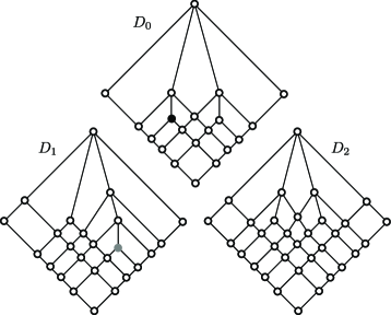
Figure 5. The process does not stop

We define a weak corner of a planar semimodular diagram $D$ as an element $x$ on the boundary of $D$ with the properties:

1. $x$ is doubly irreducible;

2. $x$ is not comparable to some $y\in D$.

If $x$ is a weak corner such that its lower cover, $x_{*}$, has exactly two covers and its upper cover, $x^{*}$, has exactly two lower covers, then we call $x$ a corner. As defined in G. Grätzer and E. Knapp [8], a planar diagram (and the corresponding lattice) is rectangular, if it has exactly one left weak corner and exactly one right weak corner, and these two elements are complementary. Slim semimodular diagrams can be obtained from slim rectangular diagrams by removing corners, one-by-one. Moreover, only slim semimodular diagrams can be obtained this way. So we get:

Corollary 3.

Slim rectangular diagrams are characterized as diagrams obtained from grids by a sequence of resections.

4. Schemes

Let $D$ be a slim semimodular diagram. By G. Grätzer and E. Knapp [6] and G. Czédli and E. T. Schmidt [3, Lemma 2], an element of $D$ has at most two covers. We also know from [3, Lemma 6] that a join-irreducible element is on the boundary of $D$.

Let $a<b$ in a planar diagram $D$, and assume that $C_{1}$ and $C_{2}$ are maximal chains in the interval $[a,b]$ such that $C_{1}-\{a,b\}$ is strictly on the left of $C_{2}$, $C_{2}-\{a,b\}$ is strictly on the right of $C_{1}$, and $C_{1}\cap C_{2}=\{a,b\}$. Then, following D. Kelly and I. Rival [9], the intersection of the right of $C_{1}$ and the left of $C_{2}$ is called a region of $D$. A region of $D$ is a planar subdiagram of $D$. Minimal regions are called cells, and cells with four vertices (and four edges) are $4$-cells. For a slim semimodular diagram $D$,

the $$4 D$$-cells and the covering squares of are the same. (1)

Our proof relies heavily on the following two lemmas, see G. Grätzer and E. Knapp [6, Lemma 7], for the first and G. Grätzer and E. Knapp [6, Lemma 6] and G. Czédli and E. T. Schmidt [3, Lemma 15], for the second.

Lemma 4.

Let $D$ be a planar lattice diagram. Then $D$ is slim and semimodular iff its cells are $4$-cells and no two distinct $4$-cells have the same bottom.

Lemma 5.

A slim semimodular diagram is distributive iff it has no cover-preserving $\mathsf{N}_{7}$.

Let $\textup{Anchor}_{i}(D)$ denote the set of anchors of $\mathsf{C}_{i}$-schemes of $D$ for $i\in\{2,3\}$. The set of interior elements of $D$, that is, the set of those elements that are not on the boundary of $D$, is denoted by $\operatorname{Inter}(D)$. Clearly,

$$\textup{Anchor}_{2}(D)\subseteq\operatorname{Inter}(D)\cap\operatorname{Mi}D\text{.}$$ (2)

As in G. Grätzer and E. Knapp [7], an $\mathsf{N}_{7}$ sublattice of $D$ is a tight $\mathsf{N}_{7}$ if the thick edges in the middle diagram of Figure 3 represent coverings. A tight $\mathsf{N}_{7}$ sublattice is always determined by its inner dual atom, we call it the centre of $\mathsf{N}_{7}$, see the black-filled element lattice in the middle of Figure 3.

Lemma 6.

Let $D$ be a slim semimodular diagram and let $u\in\operatorname{Inter}(D)\cap\operatorname{Mi}D$. Then there exists a unique tight $\mathsf{N}_{7}$ sublattice of $D$ with $u$ as the anchor. Moreover, if $[a_{l},b_{l}]$, $[u,u^{*}]$, and $[a_{r},b_{r}]$ are consecutive prime intervals of this sublattice, then this sublattice is $\{u,u^{*},a_{l},b_{l},a_{r},b_{r},a_{l}\wedge a_{r}\}$. Conversely, the center of a tight $\mathsf{N}_{7}$ sublattice always belongs to $\operatorname{Inter}(D)\cap\operatorname{Mi}D$.

Proof.

Assume that $u\in\operatorname{Inter}(D)\cap\operatorname{Mi}D$. Consider the $\mathsf{C}_{2}$-trajectory $T$ containing $[u,u^{*}]$. Since $[u,u^{*}]$ is not on the boundary of $D$, this trajectory makes at least one step to the right, to a prime interval $[a_{r},b_{r}]$. This step is a down-perspectivity since $u\in\operatorname{Mi}D$. Similarly, $T$ makes a down-perspective step to the left, to $[a_{l},b_{l}]$. By D. Kelly and I. Rival [9, Lemma 1.2], we obtain easily that $b_{l}\wedge b_{r}\leq u$. Thus $b_{l}\wedge b_{r}=b_{l}\wedge u\wedge b_{r}\wedge u=a_{l}\wedge a_{r}$, and we conclude that $\{u,u^{*},a_{l},b_{l},a_{r},b_{r},a_{l}\wedge a_{r}\}$ is a tight $\mathsf{N}_{7}$ sublattice of $D$.

Observe that a tight $\mathsf{N}_{7}$ sublattice with center $u$ is determined by those covering squares (that is, cover-preserving $\mathsf{C}_{2}^{2}$ sublattices) of this sublattice that contain $[u,u^{*}]$ as an upper prime interval. But these covering squares are $4$-cells by (1), and $[u,u^{*}]$ is the upper edge of at most two $4$-cells. Hence, apart from left-right symmetry, there is only one tight $\mathsf{N}_{7}$ sublattice with center $u$, as described in the last paragraph. This proves the first two parts of the statement. The last part is trivial. ∎

As in G. Grätzer and E. Knapp [8], a cover-preserving $m$-stacked $\mathsf{N}_{7}$ $($sublattice$)$ of $D$ is a cover-preserving sublattice isomorphic to the $(7+3m)$-element diagram given, for $m=3$, on the right of Figure 3. A cover-preserving $0$-stacked $\mathsf{N}_{7}$ is a cover-preserving $\mathsf{N}_{7}$.

Lemma 7.

Let $R$ be a cover-preserving $m$-stacked $\mathsf{N}_{7}$ sublattice of $D$. Then $R$ is a region of $D$. Furthermore, if $R^{\prime}$ a cover-preserving $m$-stacked $\mathsf{N}_{7}$ sublattice of $D$ such that $\operatorname{Inter}(R)\cap\operatorname{Inter}(R^{\prime})\neq\varnothing$, then $R^{\prime}=R$.

Proof.

Since $R$ consists of adjacent covering squares, which are $4$-cells by (1), it follows easily that $R$ is a region. Let $x_{0}\prec\cdots\prec x_{m}$ be the interior of $R$. Assume that $t\in\operatorname{Inter}(R)$. Then $t=x_{j}$, and this $j$ is recognized as follows: there is a sequence $t=t_{0}\succ\cdots\succ t_{j}$ such that

(a) $t_{j}$ has only two lower covers;

(b) the $t_{i}$ have three lower covers for $i\in\{1,\ldots,j-1\}$;

(c) $t_{i}$ is the middle lower cover of $t_{i-1}$, for $i\in\{1,\ldots,j\}$.

It follows that $t$ determines $\operatorname{Inter}(R)$, which clearly determines the whole $R$ via adjacent $4$-cells. Hence if $t\in\operatorname{Inter}(R)\cap\operatorname{Inter}(R^{\prime})$, then $R=R^{\prime}$. ∎

In view of Lemma 7, cover-preserving $m$-stacked $\mathsf{N}_{7}$ sublattices of $D$ are also called $m$-stacked $\mathsf{N}_{7}$ regions. For a meet-irreducible element $x\in D$ in the interior of $D$ define $x(0)=x$. If the meet-irreducible element $x(i)$ is already defined and $x(i)^{*}$

1. is meet-irreducible,

2. is in the interior of $D$,

3. covers exactly three elements,

then define $x(i+1)=x(i)^{*}$. The rank of $x$, $\textup{rank}_{D}(x)$, is the largest $m$ such that $x(m)$ is defined. By (2), each $x\in\textup{Anchor}_{2}(D)$ has a rank. For another description of $\textup{rank}_{D}(x)$, where $x\in\textup{Anchor}_{2}(D)$, see Corollary 9.

Lemma 8.

Let $D$ be a slim semimodular diagram. Let $x\in\textup{Anchor}_{2}(D)$ and $\textup{rank}_{D}(x)=m$. Then the following statements hold:

1. The element $x$ has exactly two lower covers.

2. For $i\in\{0,\ldots,m\}$, there exists a unique $i$-stacked $\mathsf{N}_{7}$ region $R_{i}$ of $D$ such that $\operatorname{Inter}(R_{i})=\{x=x(0)\prec\cdots\prec x(i)\}$.

3. The interior of the $\mathsf{C}_{2}$-scheme anchored by $x$ is $\operatorname{Inter}(R_{m})$.

Proof.

(i) is trivial.

To prove (ii), let $H(i)$ denote the condition “there exists a unique $i$-stacked $\mathsf{N}_{7}$ region $R_{i}$ of $D$ such that $\operatorname{Inter}(R_{i})=\{x=x(0)\prec\cdots\prec x(i)\}$”. Observe that $x$ is the center of a cover-preserving $\mathsf{N}_{7}$ sublattice $R_{0}$ by definition. It is a $0$-stacked $\mathsf{N}_{7}$ region. Since $R_{0}$ is also a tight $\mathsf{N}_{7}$ sublattice, $R_{0}$ is uniquely determined by Lemma 6. This proves $H(0)$.

Next, let $1\leq i\leq m$ and assume that $H(i-1)$ holds. Since $x(i-1)$, the anchor of $R_{i-1}$, has only one cover, it follows that $x(i)$ is the top of $R_{i-1}$; for an illustration, see the diagram on the right of Figure 3 with $i=2$. Since $x(i)$ is defined, it satisfies (a)–(c). Hence the lower covers of $x(i)$ in $D$ are exactly the same as the dual atoms of $R_{i-1}$, namely, the left dual atom $a(i)_{l}$, the anchor $x(i-1)$, and the right dual atom $a(i)_{r}$ of $R_{i-1}$. Since $x(i)\in\operatorname{Inter}(D)\cap\operatorname{Mi}D$, the right wing starting from $[x(i),x(i)^{*}]$ has to make its first step downwards to $[a(i)_{r},a(i+1)_{r}]$, where $a(i+1)_{r}$ is a uniquely determined element of $D$ because

$$\{a(i)_{r},x(i),a(i+1)_{r},x(i)\vee a(i+1)_{r}\}$$

is a $4$-cell of $D$. By left-right symmetry, we also obtain a unique $4$-cell

$$\{a(i)_{l},x(i),a(i+1)_{l},x(i)\vee a(i+1)_{l}\}.$$

Since

$$\{a(i)_{l},a(i+1)_{l},x(i),a(i)_{r},a(i+1)_{r}\}$$

generates a (unique) tight $\mathsf{N}_{7}$ sublattice by Lemma 6, it follows that

$$a(i+1)_{l}\wedge a(i+1)_{r}=a(i)_{l}\wedge a(i)_{r}.$$

This together with the fact that $R_{i-1}$ is a cover-preserving $(i-1)$-stacked $\mathsf{N}_{7}$ sublattice implies that

$$R_{i}=R_{i-1}\cup\{a(i+1)_{l},x(i)^{*},a(i+1)_{r}\}$$

is a cover-preserving $i$-stacked $\mathsf{N}_{7}$ region with interior $\{x=x(0)\prec\cdots\prec x(i)\}$. The uniqueness of this region follows from Lemma 7. Hence $H(i)$ holds for all $i\in\{0,\ldots,m\}$, proving part (ii) of the lemma.

Finally, (iii) is obvious. ∎

Corollary 9.

Let $D$ be a slim semimodular diagram, and let $x\in\textup{Anchor}_{2}(D)$. Then $\textup{rank}_{D}(x)$ is the largest number in the set

$$\{\,k\mid x\text{ is the middle atom of a $k$-stacked $\mathsf{N}_{7}$-region}\,\}.$$

5. The proof of the main result

We start with a simple consequence of Lemma 4:

Lemma 10.

1. Let $D$ be a slim semimodular diagram and let $D^{\prime}$ be obtained from $D$ by a resection at $u\in\textup{Anchor}_{3}(D)$. Then $D^{\prime}$ is also a slim semimodular diagram, $u\in\textup{Anchor}_{2}(D^{\prime})$, and up to similarity, $D$ is obtained from $D^{\prime}$ by an insertion at $u$.

2. Conversely, let $D$ be a slim semimodular diagram and let $D^{\prime}$ be obtained from $D$ by an insertion at $u\in\textup{Anchor}_{2}(D)$. Then $D^{\prime}$ is also a slim semimodular diagram, $u\in\textup{Anchor}_{3}(D^{\prime})$, and up to similarity, $D$ is obtained from $D^{\prime}$ by a resection at $u$.

The following lemma is the major step in the proof of Theorem 1. Note that the inclusions in it are actually equalities, but we do not need—and do not prove—this.

Lemma 11.

Let $D$ be a slim semimodular diagram and assume that $u\in\textup{Anchor}_{2}(D)$. Let $D^{\prime}$ denote the diagram obtained from $D$ by performing an insertion at $u$.

If $\textup{rank}_{D}(u)=0$, then

$$\textup{Anchor}_{2}(D^{\prime})\subseteq\textup{Anchor}_{2}(D)-\{u\}.$$

If $\textup{rank}_{D}(u)>0$, then

$$\textup{Anchor}_{2}(D^{\prime})\subseteq(\textup{Anchor}_{2}(D)-\{u\})\cup\{u^{*}\},$$

and $\textup{rank}_{D^{\prime}}(u^{*})=\textup{rank}_{D}(u)-1$.

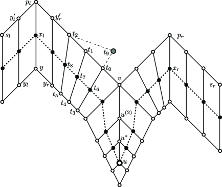
Figure 6. Insertion at $u$ ($t_{9}$ plays a role only in Case 3)

Proof.

Let $S$ denote the $\mathsf{C}_{2}$-scheme anchored by $u$. Let $I$ be the order-ideal of $D$ generated by the lower boundary of $S$ and let $F$ be order filter generated by the upper boundary of $S$. Since $I\cap S$ is the lower boundary of $S$ and $F\cap S$ is the upper boundary of $S$, planarity implies that, for all $x_{1},x_{2}\in D$,

if $$x_{1}\prec x_{2} x_{2}\in F-S x_{1}\notin F-S x_{1}\in F\cap S$$, , and , then . (3)

By Lemma 8, $u$ is the inner atom of a unique $\textup{rank}_{D}(u)$-stacked $\mathsf{N}_{7}$ region, whose top we denote by $v$, see Figure 6. (Note that we utilize that $t_{9}$ exists and is placed in the diagram as shown only in Case 3; in general, $t_{9}$ is not in $S$, and it may not be in $D$.) Let $p_{l}$ and $p_{r}$ denote the top elements of the wings. Let $s_{l}$ and $s_{r}$ denote the largest elements of the wings on the boundary of $D$. It is possible that $s_{l}=p_{l}$, or $p_{l}=v$, or $s_{r}=p_{r}$, or $p_{r}=v$.

If $x_{l}$ in Figure 6 (the element of $D^{\prime}-D$ covered by $p_{l}$) belongs to $\operatorname{Inter}(D^{\prime})$, then it has at least three lower covers in $D^{\prime}$; similarly for $x_{r}$. All the other elements of $D^{\prime}-D$ are meet-reducible. Thus $\textup{Anchor}_{2}(D^{\prime})\subseteq D$. So we have to show that every element $w$ of $D\cap\textup{Anchor}_{2}(D^{\prime})=\textup{Anchor}_{2}(D^{\prime})$ is in $\textup{Anchor}_{2}(D)$.

Since $D$ can be partitioned into

$$I\cup(F-S)\cup(F\cap S)\cup(D-(I\cup F)),$$

the condition $w\in D$ splits into four cases as to which block in this partition $w$ belongs to.

Case 1: $w\in I$. If $w\notin S$, then $w^{*}\in I\subseteq D$ by the dual of (3), the unique cover-preserving $\mathsf{N}_{7}$ sublattice is in $I\subseteq D$, and $w\in\textup{Anchor}_{2}(D)$, as required by the lemma. Therefore, we can assume that $w$ belongs to the lower boundary of $S$. Since $w\in\operatorname{Inter}(D^{\prime})\cap{\operatorname{Mi}{D^{\prime}}}$, it has to be where a wing (properly) turns down, $w=y$ in Figure 6 (or symmetrically, on the right). It has exactly two lower covers by Lemma 8. Thus these lower covers, $y_{l}$ and $y_{r}$ in Figure 6, also belong to the lower boundary of $S$. We use the notation $y_{l}^{\prime}$ and $y_{r}^{\prime}$ as in Figure 6. Lemma 6 yields that $\{y,p_{l},y_{l},y_{l}^{\prime},y_{r},y_{r}^{\prime},y_{l}\wedge y_{r}\}$ is a tight $\mathsf{N}_{7}$ sublattice of $D$. Since $y\in\textup{Anchor}_{2}(D^{\prime})$ yields that $y_{l}\wedge y_{r}\prec y_{l}$ and $y_{l}\wedge y_{r}\prec y_{r}$, this tight $\mathsf{N}_{7}$ sublattice is a cover-preserving $\mathsf{N}_{7}$ sublattice. Hence $y\in\textup{Anchor}_{2}(D)$, as required.

Case 2: $w\in F-S$. The element $w$ has exactly two lower covers, $w_{l}$ and $w_{r}$, by Lemma 8. They belong to $F$, and we have that $w_{l}\wedge w_{r}\prec w_{l}$ and $w_{l}\wedge w_{r}\prec w_{r}$. If at least one of $w_{l}$ and $w_{r}$ does not belong to $S$ (equivalently, to its the upper boundary, $F\cap S$), then $w_{l}\wedge w_{r}\in F$ by (3), whence the cover-preserving $\mathsf{N}_{7}$ sublattice determined by $w$ belongs to $F$ and $w\in\textup{Anchor}_{2}(D)$, as required. Hence we can assume that $w_{l}$ and $w_{r}$ are on the upper boundary of $S$ but $w_{l}\wedge w_{r}\notin F$. Since $w_{l}\parallel w_{r}$, the only possibility, up to left-right symmetry, is that $w=w_{l}\vee w_{r}$ equals $p_{r}$. However, this case is excluded by Lemma 8 since $p_{r}$ has at least three lower covers.

Case 3: $w\in F\cap S$. Let $w=t_{1}$ be on the upper boundary of $S$, as in Figure 6. Since it has only two lower covers by Lemma 8 and belongs to $\operatorname{Inter}(D^{\prime})$, we conclude that $t_{1}\notin\{v,p_{l},p_{r},s_{l},s_{r}\}$. Hence there are elements $t_{0},t_{2}$ in the upper boundary of $S$, in the same wing as $t_{1}$, such that $t_{0}\prec t_{1}\prec t_{2}$. We use the notation $t_{4},\ldots,t_{8}$ as in Figure 6. Consider the cover-preserving $\mathsf{N}_{7}$ sublattice in $D^{\prime}$ that is anchored by $t_{1}$. Since this sublattice is also a tight $\mathsf{N}_{7}$ sublattice in $D^{\prime}$, it is $\{t_{0},t_{1},t_{2},t_{6},t_{7},t_{8},t_{9}\}$ with rightmost dual atom $t_{9}$ by Lemma 6. Therefore, applying Lemma 6 again, the tight $\mathsf{N}_{7}$ sublattice determined by $t_{1}$ in $D$ is $\{t_{0},\dots,t_{5},t_{9}\}$. It is a cover-preserving $\mathsf{N}_{7}$ sublattice since $t_{3}\prec t_{6}$ and $t_{3}\prec t_{4}$. Thus $t_{1}\in\textup{Anchor}_{2}(D)$, as required.

Case 4: $w\in D-(I\cup F)$. Notice that $w\in\operatorname{Inter}(S)$. By Lemma 8, $w$ belongs to the interior of the unique $m$-stacked $\mathsf{N}_{7}$ region $R_{m}$ with centre $u$, where $m=\textup{rank}_{D}(u)$. Assume first that $m=0$. Then $w=u$, whence it does not belong to $\textup{Anchor}_{2}(D^{\prime})$ since it has two upper covers in $D^{\prime}$. Secondly, assume that $m>0$. Then, clearly again, $u\notin\textup{Anchor}_{2}(D^{\prime})$. Moreover, of the other elements in the interior of $S$, that is, in

$$\operatorname{Inter}({S})=\operatorname{Inter}({R_{m}})=\{\,u^{(i)}\mid 1\leq i\leq m\,\},$$

the element $u^{*}=u^{(1)}$ is the only one in $\textup{Anchor}_{2}(D^{\prime})$. ∎

Proof of Theorem 1.

Let $D$ be a diagram. If it is obtained from a slim distributive diagram by a sequence of restrictions, then $D$ is a slim semimodular diagram by Lemma 10. Conversely, assume that $D$ is a slim semimodular diagram. By virtue of Lemma 10, it suffices to show that we can obtain a slim distributive diagram from $D$ by a finite sequence of insertions. That is, we want a finite sequence $D=D_{0},D_{1},\ldots$ of diagrams such that $D_{i+1}$ is obtained from $D_{i}$ by an insertion, and the last member of the sequence is distributive. If $D_{i}$ is distributive, then it is the last member of the sequence, and we are ready. If it is non-distributive, then $\textup{Anchor}_{2}(D_{i})$ is non-empty by Lemma 5. Pick an element $u_{i}\in\textup{Anchor}_{2}(D_{i})$ such that $\textup{rank}_{D_{i}}(u_{i})$ is the smallest member of $\{\,\textup{rank}_{D_{i}}(x)\mid x\in\textup{Anchor}_{2}(D_{i})\,\}$, and perform an insertion at $u_{i}$ to obtain $D_{i+1}$. This procedure terminates in finitely many steps by Lemma 11. ∎

Proof of Corollary 3.

If we perform an insertion to obtain $D^{\prime}$ from $D$, then the weak corners of $D^{\prime}$ are the same as those of $D$, $0_{D^{\prime}}=0_{D}$, and $1_{D^{\prime}}=1_{D}$. Hence our statement follows from G. Grätzer and E. Knapp [8, Lemma 6] and the argument used in the proof of Theorem 1. ∎

There are some efficient ways to check whether a planar diagram is a slim semimodular lattice diagram; in addition to Lemma 4, see [3, Theorems 11 and 12]. The following test follows trivially from the proof of Theorem 1.

Lemma 12.

Let $D$ be a planar diagram. Construct the sequence

$$D=D_{0},D_{1},\ldots$$

as in the proof of Theorem 1. Then $D$ is a slim semimodular lattice iff the sequence terminates with a planar distributive lattice.

Remark 2 points out that the clause “as in the proof of Theorem 1” in Lemma 12 cannot be dropped.

References

- [1] G. Czédli and G. Grätzer, Planar Semimodular Lattices and Their Diagrams, Lattice Theory: Special Topics and Applications, edited by G. Grätzer and F. Wehrung, in preparation.
- [2] G. Czédli and E. T. Schmidt, The Jordan-Hölder theorem with uniqueness for groups and semimodular lattices, Algebra Universalis 66 (2011) 69–79.
- [3] G. Czédli and E. T. Schmidt, Slim semimodular lattices. I. A visual approach. Order.
- [4] G. Czédli and E. T. Schmidt, Intersections of composition series in groups and slim semimodular lattices by permutations, manuscript.
- [5] G. Grätzer, Lattice Theory: Foundation, Birkhäuser Verlag, Basel, 2011. xxix+613 pp.
- [6] G. Grätzer and E. Knapp, Notes on planar semimodular lattices. I. Construction, Acta Sci. Math. (Szeged) 73, 445–462 (2007)
- [7] G. Grätzer and E. Knapp, Notes on planar semimodular lattices. II. Congruences, Acta Sci. Math. (Szeged) 74, 37–4 (2008)
- [8] G. Grätzer and E. Knapp, Notes on planar semimodular lattices. III. Congruences of rectangular lattices, Acta Sci. Math. (Szeged) 75, 29–48 (2009)
- [9] D. Kelly and I. Rival, Planar lattices, Canad. J. Math. 27, 636–665 (1975)