A Corona Australis cloud filament seen in NIR scattered light

Abstract

Context. The dust is an important tracer of dense interstellar clouds but its properties are expected to undergo changes affecting the scattering and emitting properties of the grains. With recent Herschel observations, the northern filament of the Corona Australis cloud has now been mapped in a number of bands from 1.2 $\mu$m to 870 $\mu$m. The data set provides a good starting point for the study of the cloud over several orders of magnitude in density.

Aims. We wish to examine the differences of the column density distributions derived from dust extinction, scattering, and emission, and to determine to what extent the observations are consistent with the standard dust models.

Methods. From Herschel data, we calculate the column density distribution that is compared to the corresponding data derived in the near-infrared regime from the reddening of the background stars, and from the surface brightness attributed to light scattering. We construct three-dimensional radiative transfer models to describe the emission and the scattering.

Results. The scattered light traces low column densities of $A_{\rm V}\sim$1^m better than the dust emission, remaining useful to $A_{\rm V}\sim 10-15^{\rm m}$. Based on the models, the extinction and the level of dust emission are surprisingly consistent with a sub-millimetre dust emissivity typical of diffuse medium. However, the intensity of the scattered light is very low at the centre of the densest clump and this cannot be explained without a very low grain albedo. Both the scattered light and dust emission indicate an anisotropic radiation field. The modelling of the dust emission suggests that the radiation field intensity is at least three times the value of the normal interstellar radiation field.

Conclusions. The inter-comparison between the extinction, light scattering, and dust emission provides very stringent constraints on the cloud structure, the illuminating radiation field, and the grain properties.

1 Introduction

The interstellar clouds are hierarchical structures where gravitationally bound prestellar cores are found on the smallest scales. The study of the dense clouds is largely motivated by this connection to star formation. The filamentary nature of interstellar clouds and the possible connection between filaments and star formation has been known for a long time (e.g. Barnard 1919; Fessenkov 1952; Elmegreen & Elmegreen 1979; Schneider & Elmegreen 1979; Bally et al. 1987). The recent ground-based studies and Herschel surveys have shown cloud filaments in exquisite detail (Miville-Deschênes et al. 2010; André et al. 2010; Arzoumanian et al. 2011; Hill et al. 2011; Juvela et al. 2010) and have demonstrated that pre-stellar cores and protostars are preferentially located along these structures (André et al. 2010; Men’shchikov et al. 2010; Juvela et al. 2012). Filaments are a natural outcome of interstellar turbulence (e.g. Padoan & Nordlund 2011), with further contributions from immediate triggering by supernova explosions and the radiation and stellar winds from massive stars. However, some filaments may also be formed directly by gravitational processes, as have been modelled in numerous cosmological simulations, and in other theoretical studies (e.g. Burkert & Hartmann 2004). The filaments should fragment as dictated by the local Jeans condition, a process addressed by many theoretical studies (Inutsuka & Miyama 1997; Myers 2009). In addition to the pure compressive instability, also the so-called sausage instability may sometimes play an additional role (see Fischera & Martin 2012; McLeman et al. 2012). Although the morphology of all the star-forming clouds is not predominantly filamentary (Juvela et al. 2012), a global picture of star formation is emerging, where the turbulence creates filaments, the filaments become gravitationally unstable and subsequently fragment forming the cores that may still fed by material flowing in along the filaments. Low mass stars can be found in individual filaments while high mass stars are preferentially born at the intersections of several filaments. This scenario is supported by the observations made within the Herschel Gould Belt survey (e.g. André et al. 2010; Könyves et al. 2010; Men’shchikov et al. 2010) and other Herschel programs (Molinari et al. 2010; Schneider et al. 2010; Nguyen Luong et al. 2011; Hill et al. 2011; Schneider et al. 2012; Juvela et al. 2012) as well as by numerical simulations (Padoan & Nordlund 2011; Vázquez-Semadeni et al. 2011; Klessen 2011; Bonnell et al. 2011).

To determine the initial conditions for the star formation to occur, we need to measure the physical properties of the clouds, the filaments, and the cores. The mass distributions of the clouds can be measured with a number of methods. This is fortunate because each method suffers from different sources of uncertainty.

The dense clouds have been traditionally mapped in molecular lines. Line observations are invaluable because of the information they give on the physical state, kinematics, and chemistry of the clouds (Bergin & Tafalla 2007). On the other hand, they do not always provide reliable or consistent estimates of the mass distribution. The line intensity depends on the local physical conditions, mainly density and temperature, and the chemical abundances. If the lines are not optically thin, the radiative transfer effects introduce additional uncertainty.

For the above reasons – and because of the development in detector technology and the appearance of new ground-based, balloon-borne, and space-borne facilities – the thermal dust emission has become important as a tracer of the densest clouds. Observations of the dust at submm wavelengths are of particular interest because they are sensitive to the emission of the cold dust that may have been missed in earlier far-infrared studies. With the knowledge of dust temperature and dust opacity, the column density can be estimated. However, the colour temperature obtained from observations is known to be a biased estimator of the average dust temperature (Shetty et al. 2009b; Juvela & Ysard 2012b) and additionally the value of the dust opacity is uncertain. Furthermore, there are clear indications that the dust opacity is not constant, the variations being a likely consequence of grain coagulation and aggregation processes (Cambrésy et al. 2001; del Burgo et al. 2003; Kramer et al. 2003; Lehtinen et al. 2007). Similarly, the spectral index appears to vary from region to region and this increases the uncertainty of the colour temperature and column density estimates. The observations point to a negative correlation between the colour temperature $T_{\rm d}$ and the observed spectral index $\beta_{\rm Obs}$ (Dupac et al. 2003; Désert et al. 2008; Anderson et al. 2010; Paradis et al. 2010; Veneziani et al. 2010; Planck Collaboration et al. 2011b; Arab et al. 2012). Such variations can affect the accuracy of the column density estimates derived from the dust emission. However, the evaluation of errors is complicated by the observational noise (also through its effect on the $T_{\rm d}-\beta_{\rm Obs}$ relation, see Shetty et al. (2009a); Juvela & Ysard (2012a) and the unknown line-of-sight temperature variations (Shetty et al. 2009b; Juvela & Ysard 2012a). One of the main advantages of submm observations of dust emission is the large range of column densities probed. With the Herschel satellite SPIRE instrument (Griffin et al. 2010) one can probe regions from $A_{\rm V}\sim 1^{\rm m}$ to $A_{\rm V}\sim 100^{\rm m}$ with spatial resolution of $\sim 30\arcsec$ . However, the accuracy will depend on the line-of-sight temperature variations and other opacity effects (Malinen et al. 2011).

Complementary information can be obtained from near-infrared (NIR) observations, from reddening of the light of background stars, and from the measurement of the scattered light. The observed near-infrared colour excesses can be converted to column density or to provide estimates of the visual extinction $A_{\rm V}$ using techniques such as the NICER algorithm (Lombardi & Alves 2001). The calculations are based on the assumption that the average intrinsic colour of the stars is constant and, therefore, reliable estimates are obtained only as an average over a number of stars. Therefore, the extinction must be estimated for larger pixels, as an average over $\sim$10 or more background stars. This reduces the resolution of the extinction maps and can cause bias in the presence of strong $A_{\rm V}$ gradients. With dedicated observations it is possible to achieve a spatial resolution of some tens of arc seconds, which is comparable to the resolution of the submm surveys. The range of $A_{\rm V}$ values probed extends from $A_{\rm V}\sim 1^{\rm m}$ to $\sim 40^{\rm m}$, depending on the stellar density and the depth of the observations.

If the NIR observations are made using an ON-OFF mode the diffuse signal is preserved and it is possible to measure the light scattered by the same dust particles that are responsible for the NIR extinction. If the cloud is optically thin at the observed wavelengths and if the cloud does not include local radiation sources, the signal will be proportional to the column density (Juvela et al. 2006). The main advantage of the surface brightness measurement is the high, potentially $\sim 1\arcsec$ spatial resolution. Even in normal NIR observations at mid-Galactic latitudes, the scattered light will provide better resolution than similar observations of the background stars. The method remains useful in the range $A_{\rm V}=1$–$15^{\rm m}$. At higher column densities the signal saturates and the surface brightness will depend on the structure of the cloud. With multiwavelength measurements (e.g., J, H, and K bands) it becomes possible to use the intensity ratios to measure and to partially correct for the saturation of the signal (Juvela et al. 2006, 2008, hereafter Paper I and Paper II, respectively). The observed surface brightness depends on the grain properties and upon the intensity of the radiation field at the location of the cloud. Therefore, combining surface brightness data with other column density tracers one can also provide constraints to these parameters.

In this paper we will examine a filament in the northern end of the Corona Australis molecular cloud. The filament contains a dense clump with a central $A_{\rm V}$ previously estimated to be at least $\sim 30^{\rm m}$. The source has been studied with the help of NIR observations using background stars and the scattered light (Juvela et al. 2006, 2008, 2009). The region has now been mapped with the Herschel satellite and these data provide the opportunity to measure the structure of the central part of the filament where the column density was too high to enable reliable estimates either with the NICER or with the surface brightness (scattered light) methods. This provides an excellent opportunity to compare the performance of the three column density tracers and to use the comparison to look for indications for changes in the dust properties.

The structure of the paper is the following: In Sect. 2 we describe the observations and the main properties of the data. In Sect. 3 we present the direct results derived from each data set and make the first comparison between the column density estimates. We continue by constructing radiative transfer models for the NIR data and the sub-millimetre data separately. These calculations are described and compared in Sect. 4. Our final conclusions are given in Sect. 5.

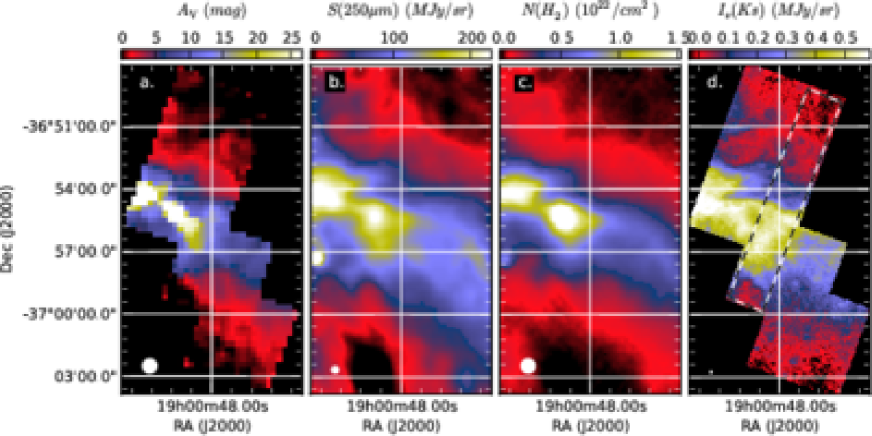
Figure 1: A cross section of the northern Corona Australis filament according to the different tracers. Maps are shown for the visual extinction derived from the reddening of the background stars (frame $a$, 40$\arcsec$ resolution), the 250 $\mu$m surface brightness (frame $b$, 18$\arcsec$ resolution), the column density derived from the Herschel data (frame $c$, 40$\arcsec$ resolution), and the intensity of the scattered light in the $K_{s}$ band (frame $d$, 4$\arcsec$ resolution). For the plot the data have been adjusted so that the median signal is zero within the reference area located in the northern end of the maps (see text). The dashed rectangle in frame $d$ denotes the area that will be used to measure the filament profile.

2 The observations

2.1 Near-infrared data

The NIR observations were made with the SOFI instrument on the NTT telescope, Chile. All observations were carried out in ON-OFF mode. The northern part, an area of $4\arcmin\times 8\arcmin$ was observed in 2006. The integration times on the ON-fields were 1.0 hour in the J band, 1.5 hours in the H band, and 4.5 hours in the Ks band. The map was extended in June 2007 with two $4\arcmin\times 4\arcmin$ fields that cover the southern side of the filament. The integration times were 1.5 hours for the Ks band and 0.5 hours in the J and H bands. On the basis of the 2MASS data (Skrutskie et al. 2006), the OFF field was estimated to have an extinction below $A_{\rm V}=0.5^{\rm m}$. For the details of the observations, see Juvela et al. (2008) and Juvela et al. (2009).

The observations were calibrated using the 2MASS stellar photometry and that calibration was carried over to the surface brightness. For the final surface brightness map the southern ON fields were mosaiced together with the northern part, this requiring a small additive adjustment. The observations do not provide an absolute measure of the surface brightness. Therefore, we present the results relative to the signal within a $1\arcmin$ diameter aperture centred at coordinates $\alpha_{\rm 2000}$=19^h0^m43.5^s, $\delta_{\rm 2000}$=-36$\degr$49$\arcmin$36$\arcsec$ (see Fig. 1d). Based on the 2MASS data, the visual extinction in this reference area is $\sim 1.8^{\rm m}$ (see Juvela et al. 2009).

In Juvela et al. (2008) the NICER method (Lombardi & Alves 2001) was used to convert the measured stellar colour excesses to estimates of extinction. This extinction map is reproduced in Fig. 1a with $A_{\rm V}$ values relative to the above described reference area. The frames b and c show for the same area the 250 $\mu$m surface brightness and the column density derived from the Herschel data.

2.2 Herschel observations

The Corona Australis cloud has been mapped as part of the Herschel Gould Belt Survey (André et al. 2010). The entire cloud is covered by parallel mode maps that also cover the northern filament. The observation were made with the PACS instrument (Poglitsch et al. 2010) at wavelengths 70 $\mu$m and 160 $\mu$m and with the SPIRE instrument (Griffin et al. 2010) at wavelengths 250 $\mu$m, 350 $\mu$m, and 500 $\mu$m. The observation consist of two orthogonal scans with observation identifiers 1342206677 and 1342206678. We use data provided by the Herschel Gould Belt Consortium. We use the SPIRE maps produced with the naive mapping routine in HIPE software (Ott 2010). The 160 $\mu$m PACS map is made using Scanamorphos v. 16 (Roussel 2011, submitted), starting from data processed to level 1 in HIPE. The 70 $\mu$m data were not used, since at that wavelength the emission is not produced by the large dust grains that are responsible for the longer wavelength emission. For the Herschel data the zero point of the intensity scale was estimated by comparison with data from the Planck satellite survey (see Bernard et al. 2010). These zero points are used in the derivation of the column density estimates. However, in the plots (e.g., Fig.1b) and in comparison with the other tracers, the zero level is set using the reference area described in Sect. 2.1.

2.3 Laboca 870 $\mu$m data

The Corona Australis filament was mapped in 2008 with the APEX/LABOCA instrument. This instrument operates at a wavelength of 870 $\mu$m, and has the beam size $\sim 19\arcsec$. Observations consist of $\sim 30\arcmin$ long scans that were made perpendicular to the filament, and at up to 30 degree angles relative to the normal of the filament. The observations were reduced using the Boa program, version 1.11 and the calibration checked with planet observations and with the help of the source S CrA that is located immediate south-east of the area covered by the NIR data. The final noise level in the central part of the map is better than 20 mJy/beam. For details of the Laboca observations, see Juvela et al. (2009).

2.4 Mid-infrared data

The area was mapped in Spitzer guaranteed time programs with both the IRAC instrument (3.6, 4.5, 5.8, and 8.0 $\mu$m) and the MIPS instrument (24, 70, and 160 $\mu$m). The MIPS data were already compared to the LABOCA and NIR data in Juvela et al. (2009). The images of the four IRAC bands are shown in Fig.2. The 5.8 and 8.0 $\mu$m surface brightness is affected by the nearby stars and does not trace the column density. The 3.6 and 4.5 $\mu$m data will be used in Sect. 3.3 check for signs of enhanced mid-infrared scattering.

We will use also data from the WISE survey that have recently become public. The WISE data includes the wavelengths of 3.4, 4.6, 12, and 22 $\mu$m (Wright et al. 2010).

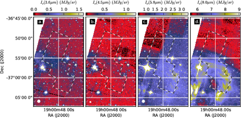
Figure 2: Spitzer IRAC maps at 3.6, 4.5, 5.8, and 8.0 $\mu$m. The dashed line shows the outline of the regions covered by NIR observations. The brightest star east of the area covered by NIR observations is S CrA. The other bright source in the southern end of the images (at $\delta_{\rm 2000}=-37\degr 3\arcmin 42\arcsec$) corresponds to the blended image of the stars HD 176269 and HD 176270.

3 The results

3.1 The column densities

3.1.1 Column density derived from the Herschel data

The Herschel measurements of submm dust emission were converted to column density using the usual procedure that assumes a constant dust temperature along the line of sight and a constant dust opacity everywhere within the mapped area. For each map pixel, the observed intensities $I_{\nu}$ at 160 $\mu$m, 250 $\mu$m, 350 $\mu$m, and 500 $\mu$m were fitted with a modified black body curve $B_{\nu}(T_{\rm C})\nu^{\beta}$ to determine the colour temperature $T_{\rm C}$. With knowledge of the dust opacity $\kappa$ (and the spectral index $\beta$) the fit determines the column density. The column density of the molecular hydrogen can be written formally as:

$$N({\rm H}_{2})=\frac{I_{\nu}}{B_{\nu}(T)\kappa\mu m_{\rm H}},$$ (1)

where $T$ is the assumed temperature, here equal to the colour temperature $T_{\rm C}$, $\mu$ is the average particle mass per hydrogen molecule, and the dust opacity $\kappa$ is given relative to the gas mass.

In the analysis, the surface brightness maps are convolved to a common resolution of $40\arcsec$ resolution before the determination of $T_{\rm C}$ and $N$(H₂). The spectra are modelled assuming a constant value of the spectral index, $\beta=2.0$ and a dust opacity $\kappa=$0.1 cm²/g ($\nu$/1000 GHz)^β that is applicable to high density environments (Hildebrand 1983; Beckwith et al. 1990). The same opacity law has been adopted in several papers on Herschel results (André et al. 2010; Könyves et al. 2010; Arzoumanian et al. 2011; Planck Collaboration et al. 2011a; Juvela et al. 2012). However, for any particular sources, the values of these parameters are not known to high precision and both the $\beta$ and the $\kappa$ values introduce an uncertainty in the column density that may be several tens of per cent.

The calculated column density map is shown in Fig. 1c and the colour temperature map is shown separately in Fig. 3. The minimum temperature at the location of the densest clump is $T_{\rm C}\sim 12.5$ K. This value is obtained using the total intensity (i.e., the original zero point of the Herschel maps) without subtracting the signal in the local reference area (see Sect. 2.2).

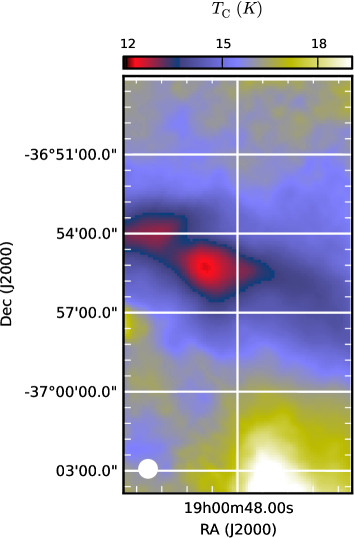
Figure 3: The map of the dust colour temperature $T_{\rm C}$.

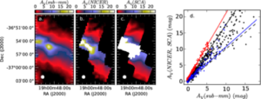
Figure 4: A comparison of the $A_{\rm V}$ estimates derived from the sub-millimetre emission (frame $a$, the column density converted to $A_{\rm V}$ with the assumptions listed in the text), the reddening of the background stars (frame $b$), and the dust scattering (frame $c$). All maps have been convolved to a common resolution of 40$\arcsec$. The frame $d$ shows the NICER $A_{\rm V}$ estimates (black points) and the estimates $A_{\rm V}^{\rm SCA}$ derived from the NIR surface brightness as the function of the values from sub-millimetre data. The blue and the red points are, respectively, the $A_{\rm V}^{\rm SCA}$ values north and south of declination $-$36$\degr$55$\arcmin$. The solid lines are least squares fits to the respective data points. The dashed line indicates the one-to-one relation.

3.1.2 The $A_{\rm V}$ maps from NIR data

The extinction derived from the colour excesses of the background stars was calculated using the NICER method (Lombardi & Alves 2001). The resulting maps of visual extinction, $A_{\rm V}^{\rm NICER}$ have a resolution of 30$\arcsec$. A similar map with a 20$\arcsec$ resolution has already been presented by Juvela et al. (2008). Here we settle for a more reliable but a slightly lower initial resolution of 30$\arcsec$ because the data will later be compared to lower resolution column density maps derived from the Herschel data. The extinction map covers the whole area included in the NIR observations (see Fig.1a). The maximum extinction values are $\sim$33^m but because no background stars are visible at the centre of the dense clumps within the filament, this is only a lower limit. Furthermore, because of the strong $A_{\rm V}$ gradients the values near the filament centre may be biased downwards (see Juvela et al. 2008).

In Juvela et al. (2008) and Juvela et al. (2009) the surface brightness, assumed to consist only of scattered light, was converted to column density assuming analytical formulas $I_{\nu}\sim a_{\nu}(1-exp(-b_{\nu}A_{\rm V}))$ for the relation between the surface brightness and the extinction. This resulted in an extinction map $A_{\rm V}^{\rm SCA}$ that was consistent with the $A_{\rm V}^{\rm NICER}$ values up to $\sim 10^{\rm m}$ but gave higher values in the range of 10–15^m. It was not clear which of the two extinction estimates was more robust although simulations indicated that most of the difference could be explained by bias in $A_{\rm V}^{\rm NICER}$. When the extinction approaches 20^m the surface brightness is strongly saturated and the simple analysis method adopted in Juvela et al. (2008, 2009) leads to diverging values. The saturation of the surface brightness and the dip at the centre of the dense clump are evident even in the $K_{s}$ band (see Fig.1d) where, compared to the $V$ band the optical depth is lower by close to a factor of ten. This alone confirms that the central $A_{\rm V}$ must be higher than 20^m. As in Juvela et al. (2008), the spatial resolution of this initial $A_{\rm V}^{\rm SCA}$ map is 10$\arcsec$.

3.1.3 The comparison of the column density maps

In Fig. 4 we compare the column density estimates from the submm emission, the reddening of the background stars (the NICER method by Lombardi & Alves (2001)), and from the NIR surface brightness data (Juvela et al. 2009).

For easier comparison, the Herschel estimates of $N$(H₂) were also converted to units of visual extinction, $A_{\rm V}^{\rm sub-mm}$. The conversion was done using the canonical relation $N$(H₂)=$0.94\times 10^{21}A_{\rm V}$ (Bohlin et al. 1978). That relation was determined for more diffuse lines of sight and may not be representative of the present field, but does at least provide a convenient point of reference. The map of $A_{\rm V}^{\rm sub-mm}$ (a scaled version of Fig. 1c) is shown in Fig. 4a. The map of $A_{\rm V}^{\rm NICER}$ was convolved to the resolution of 40$\arcsec$. We have masked the areas near the borders of the observed area where the result of the convolution is not well defined (where more than 10% of the convolving beam falls outside observed region). The $A_{\rm V}^{\rm NICER}$ map is shown in Fig. 4b. In the case of the NIR surface brightness, $A_{\rm V}^{\rm SCA}$ values remain undefined in the central part of the filament where the simple analytical solution diverges. In the area where the $A_{\rm V}^{\rm SCA}$ estimates exceed 25^m, before making the convolution, the data were replaced with values read from the NICER map. After the convolution, those areas are masked from the subsequent analysis (Fig. 4c). In the plots Fig. 4a–c the map zero points were set using the common reference region (see 2.1).

The three $A_{\rm V}$ maps are morphologically very similar at low and intermediate extinctions. In the lowest $A_{\rm V}$ regions the absolute value of the visual extinction is of order of 1–3^mag. At those diffuse lines-of-sight the correspondence is best between the two NIR-derived maps because one is close to the sensitivity of the sub-millimetre data (or because the sub-millimetre maps may be affected by minor baseline uncertainties).

Figure 4d confirms the good correspondence between the tracers. Below $A_{\rm V}^{\rm sub-mm}=10^{\rm m}$ the correlation coefficients coefficient is 0.96 for the $A_{\rm V}^{NICER}$–$A_{\rm V}^{\rm sub-mm}$ relation with a least squares line $A_{\rm V}^{NICER}$=-0.11+1.76$\times A_{\rm V}^{\rm sub-mm}$. For the relation $A_{\rm V}^{SCA}$–$A_{\rm V}^{\rm sub-mm}$ the correlation coefficient is $r=$0.86 but the presence of two different relations is evident. In the northern half of the map (blue points in Fig. 4d) the least squares fit gives a relation $A_{\rm V}^{SCA}$=0.15+1.05$\times A_{\rm V}^{\rm sub-mm}$ with a correlation coefficient of $r=$0.95. The slopes are consistent with the results presented by Juvela et al. (2008) where the $A_{\rm V}^{SCA}$ was below the $A_{\rm V}^{NICER}$ values up to $\sim 10^{\rm m}$ while the situation was reversed at higher $A_{\rm V}$. On the southern side the relation is $A_{\rm V}^{SCA}$=0.81+2.03$\times A_{\rm V}^{\rm sub-mm}$ with an even higher correlation coefficient, $r$=0.98. The main difference compared to the northern side is the much steeper slope of the relation. The northern and the southern fields were calibrated separately, but a factor of two difference in the calibration is very improbable. Furthermore, the surface brightness values decrease to zero both at the southern and northern edges of the maps and the surface brightness values were matched at the centre when the fields were mosaiced together. Therefore, there is no room for an over 60% multiplicative error in the relative calibration. The difference is an indication of a change in the local NIR radiation field. Assuming that the grain properties are the same, and ignoring the fact that the scattering is mostly in the forward direction, this would suggest that the radiation field intensity is at least 50% higher on the southern side of the filament. This is qualitatively consistent with the conclusions of Juvela et al. (2009) that were based on the morphology of the NIR and the Spitzer dust emission maps.

The average ratios $A_{\rm V}^{SCA}$/$A_{\rm V}^{\rm sub-mm}$ and $A_{\rm V}^{NICER}$/$A_{\rm V}^{\rm sub-mm}$ are $\sim 1.5$ or higher. The interpretation of $A_{\rm V}^{SCA}$ is affected by the uncertainty of the intensity of the interstellar radiation field (ISRF) but that does not influence $A_{\rm V}^{NICER}$. It would thus appear that ISRF is not very different from Mathis et al. (1983) values north of the filament but are clearly elevated on the southern side. The $A_{\rm V}^{\rm sub-mm}$ values appear to be too low by almost a factor of two. Part of the difference could be caused the assumed scaling between N(H₂) and $A_{\rm V}$, but it is clear that especially the value of the dust opacity $\kappa$ has a large uncertainty. The $A_{\rm V}^{\rm sub-mm}$ values were derived with an opacity of $\kappa=$0.1 cm²/g ($\nu$/1000 GHz)^β that is higher than the value found in diffuse regions. Boulanger et al. (1996) derived for high latitude clouds a value of $\kappa(850\,\mu{\rm m})$=0.005 cm² g^-1 which is $\sim$40% of the value given by the previous formula. Thus, with the diffuse medium $\kappa$ the $A_{\rm V}^{\rm sub-mm}$ values would rise above the $A_{\rm V}^{NICER}$ values. This suggests that the actual value of $\kappa$ should be somewhere in between. However, it is also known that the colour temperature used in Eq. 1 overestimates the mass averaged dust temperature and may lead to the underestimation of the column densities (see Shetty et al. 2009b; Malinen et al. 2011; Ysard et al. 2012; Juvela & Ysard 2012b). If this effect can be quantified, it becomes possible to increase the lower limit the dust opacity. This is possible only with modelling and we will return to this question in Sect. 4.

3.2 The NIR and sub-millimetre profiles of the filament

We measure the profile of the filament using the three tracers available to us. The sub-millimetre emission is the only one that, at least in principle, is capable of probing the column density distribution across the whole filament. Good $A_{\rm V}^{NICER}$ estimates are missing for a small central part where no background stars are visible (roughly the white area in Fig. 4a). The NIR surface brightness data are reliable only in regions of less than $A_{\rm V}\sim 10^{\rm m}$. Because we want to compare all the tracers, we concentrate on the narrow region that is marked with dashed lines in Fig. 1d. We calculate the one-dimensional profile along the main axis of that region, averaging the data in the perpendicular direction.

Figure 5 shows the resulting column density profiles that, like in Fig. 4, are converted to units of visual extinction. The first frames show the data at the original resolution (cf Fig. 4). There is an offset between the maps. In the northern end the $A_{\rm V}^{\rm sub-mm}$ decreases below 0.5^m while the other maps are, based on the large scale 2MASS extinction maps, were set at $\sim 2^{\rm m}$. This is not likely to be caused by an uncertainty in the zero point of the Herschel surface brightness data. The missing $\sim 1.5^{\rm m}$ corresponds to a 250 $\mu$m surface brightness of $28$ MJy sr^-1, this assuming a temperature of $T_{\rm d}=17$ K and a dust opacity of $\kappa=0.005\times(\lambda/850$ $\mu$m)^-2 cm² g^-1 (see Sect. 3.1.3). Such a surface brightness offset would be comparable to the minimum signal found in the northern part of examined area. Figure 5 again shows the discrepancy in the $A_{\rm V}^{\rm SCA}$ estimates. On the northern side these follow closely the shape of the $A_{\rm V}^{\rm NICER}$ curve but they are significantly higher in the southern end. In the plot we have not included the $A_{\rm V}^{\rm SCA}$ values for the central filament, $A_{\rm V}^{\rm SCA}>10^{\rm m}$, because of their large uncertainty near the region where the surface brightness saturates.

The frame $b$ of Fig. 5 shows the same data convolved to a common resolution of 40$\arcsec$. The value at the offset of $10\arcmin$ has been subtracted, and the $A_{\rm V}^{\rm sub-mm}$ values have been scaled by a factor of 1.3. With this scaling, the column density estimates are very consistent on the northern slope. For $A_{\rm V}^{\rm NICER}$ and the scaled version of $A_{\rm V}^{\rm sub-mm}$ the match is good up to $A_{\rm V}=15^{\rm m}$. However, the peak of $A_{\rm V}^{\rm NICER}$ is almost one minute of arc south of the $A_{\rm V}^{\rm sub-mm}$ maximum. The $A_{\rm V}^{\rm sub-mm}$ profile is strongly skewed towards the north and rough agreement is found again in the south end of the map. If we trust the NICER map, both $A_{\rm V}^{\rm SCA}$ and $A_{\rm V}^{\rm sub-mm}$ show deviations on the south side of the filament and qualitatively both features could be affected by the asymmetry of the radiation field. Figure 5a shows as dotted lines the minimum and maximum $A_{\rm V}^{\rm NICER}$ along the stripe for which the other curves show the average value. These indicate that there is a strong $A_{\rm V}$ gradient perpendicular to the stripe and parallel to the filament, especially close to the high column density clump. This could cause significant bias in $A_{\rm V}^{\rm NICER}$ (see Juvela et al. 2008) but cannot explain all the differences between $A_{\rm V}^{\rm NICER}$ and $A_{\rm V}^{\rm sub-mm}$, neither in the levels nor in the profiles.

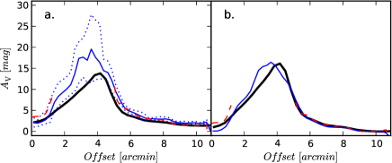
Figure 5: The column density profiles for the region marked with a dashed rectangle in Fig. 1d. The left hand frame shows the $A_{\rm V}^{sub-mm}$ (thick black line), $A_{\rm V}^{NICER}$ (thin blue line), and $A_{\rm V}^{SCA}$ (dashed red line, excluding the central filament where the NIR emission becomes partly saturated) at the original resolution (40$\arcsec$, 30$\arcsec$, and 10$\arcsec$, respectively) without scaling. The x-axis is the offset along the stripe, from south to north. The dotted lines are the profiles of the maximum and minimum $A_{\rm V}^{\rm NICER}$ along the stripe. The right hand frame shows the same data at a common 40$\arcsec$ resolution, with values set to zero at offset 10$\arcmin$ (additive correction). The $A_{\rm V}^{sub-mm}$ values have been scaled by a factor 1.3 to match the other curves on the northern side of the filament.

3.3 Mid-infrared profiles

Although we will not attempt to model the mid-infrared data of the Corona Australis cloud (Sect. 4) it is also useful to examine the Spitzer IRAC and the WISE satellite observations of the filament. Figure 6 compares the 3.6 $\mu$m and 4.5 $\mu$m Spitzer IRAC profiles with the scattered light and the extinction derived from the Herschel data.

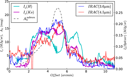
Figure 6: The mid-infrared profiles of the Corona Australis filament. The offsets are the same as in Fig. 5. In addition to the Spitzer 3.6 $\mu$m and 4.5 $\mu$m data (blue and lines, respectively, and the right hand y-axis) the figure includes the profiles for the scattered light in the $H$ and $Ks$ bands (cyan and magenta lines, left hand axis) and the $A_{\rm V}$ derived from the Herschel observations (black dashed line, left axis).

The mid-infrared profiles show some resemblance to the NIR bands but follow more closely the column density profile of the filament as derived from the sub-millimetre observations. In particular, the 4.5 $\mu$m emission peak coincides with the location of the column density maximum derived from the Herschel data. Compared to the estimated column density, both the 3.6 $\mu$m and 4.5 $\mu$m data show significantly higher intensity levels on the south side. We compared the Spitzer and WISE data at the wavelengths of 3.4 $\mu$m and 4.6 $\mu$m. The WISE measurements are in complete agreement with the Spitzer data at the corresponding wavelengths except for the 3.4 $\mu$m intensity that is slightly lower in WISE at the location column density peak ($\sim$0.18 MJy/sr vs. 0.21 MJy/sr) so that the intensity remains almost flat between offsets 3.0$\arcmin$-5.5$\arcmin$. Further outside the filament, the Spitzer ratio 3.6 $\mu$m/4.5 $\mu$m and the WISE ratio 3.4 $\mu$m/4.6 $\mu$m show some increase. This could be caused by the effect the optically thick filament has on the local radiation field but the quantification of these effects would require separate modelling.

The mid-infrared data have revealed in many dense cloud cores the presence of the “coreshine” phenomenon where the emission at $\sim$3.5 $\mu$m becomes brighter relative to the emission at $\sim$4.5 $\mu$m (Steinacker et al. 2010; Pagani et al. 2010). The changes are interpreted as a sign of an increase of dust grain sizes that leads to enhanced light scattering at wavelengths beyond 3 $\mu$m. The first detection of coreshine was made in the cloud LDN 183 using Spitzer data (Steinacker et al. 2010). Further detections have subsequently been made with WISE observations (Juvela et al. 2012) but LDN 183 remains the best example of the phenomenon. Figure 6 shows significant increase of the 3.6 $\mu$m/4.5 $\mu$m ratio but only south of the column density peak. This is thus probably caused by a change of the radiation field rather than by grain growth. Regarding the overall asymmetry with respect to the filament centre, the 3.5 $\mu$m profile is rather similar to that of the $K$ band.

Table 1: The radiative transfer models.

Radiation field	Dust model	Figures	Notes
isotropic, $\chi=2$	OH	Fig. 7
isotropic, $\chi=3$	OH	Fig. 7
isotropic, $\chi=4$	MWD	Figs. 8, 13
isotropic, $\chi=4$	OH	Figs. 8, 9, 13, 16
anisotropic, $\chi=3+1^{a}$	OH	Figs. 10, 11, 14
anisotropic, $\chi=3+1^{a}$	MWD	Fig. 14
isotropic, $\chi=4$	MWD	Fig. 15	$n\times 2^{b}$
anisotropic, $\chi=3+1$	MWD	Fig. 15	$n\times 2^{b}$

^a Ratio 3:1 between isotropic background and additional radiation from the south-eastern direction.

^b Densities twice the values obtained from the modelling of sub-millimetre emission.

4 Radiative transfer models

4.1 Model of the sub-millimetre emission

We construct a three-dimensional model to explain the Herschel observations of 160 $\mu$m, 250 $\mu$m, 350 $\mu$m, 500 $\mu$m. In the present paper we examine only the main effects, including the possibly anisotropic radiation field, using two dust models. The first model corresponds to $R_{\rm V}$=5.5 and is described in Draine (2003). In the following, this dust model is called MWD. As a point of comparison, we use the Ossenkopf & Henning (1994) dust model (in the following, the model OH) for coagulated grains with thin ice mantles that have accreted in $10^{5}$ years at a density of $10^{5}$ cm^-3. At wavelengths below 1 $\mu$m we adopt the short wavelength extension discussed in Stamatellos & Whitworth (2003). The dust models differ with respect to the sub-millimetre spectral index $\beta$ that, measured between 250 $\mu$m and 500 $\mu$m is $\sim 2.1$ for the MWD dust model and 1.76 for the OH model. The optical depth ratios for extinction $\tau(0.55\,\mu{\rm m})/\tau(350\,\mu{\rm m})$ are 1760 and 2080 for MWD and OH, respectively. Detailed studies of the possible variations of the dust properties are deferred to a later paper. Here the two models are used only to test the sensitivity of the results to the actual dust properties. The dust emission is calculated with our radiative transfer program (Juvela & Padoan 2003; Juvela 2005). The program uses Monte Carlo simulation to determine the radiation field intensity at each position within the model cloud. This information is used to determine the distribution of dust temperatures. The line-of-sight integration of the radiative transfer equation then results in synthetic surface brightness maps that are calculated for each of the observed wavelengths.

To avoid edge effects near the boundaries of the area covered by the NIR data, we include in the model a larger area than that shown in Fig. 1. The modelled area is $10\arcmin\times 10\arcmin$, centred at coordinates $\alpha_{\rm 2000}$=19^h0^m54.3^s, $\delta_{\rm 2000}$=-36$\degr$55$\arcmin$22$\arcsec$. The model will be adjusted to reproduce the observed 350 $\mu$m data. This is accomplished by having as free parameters the column densities corresponding to each map pixel. The optimisation will determine the column density for each line-of-sight and thus the mass distribution in the plane of the sky. In principle, the solution should be unique for any combination of the external radiation field and dust properties. However, the line-of-sight density distribution must be fixed for this modelling. According to Fig. 5 in the plane of the sky the FWHM of the column density distribution is $\sim 2.5\arcmin$ perpendicular to the filament. For the assumed distance of 130 pc (Marraco & Rydgren 1981) this corresponds to a filament width of $\sim 0.1$ pc. We assume that the filament is approximately cylindrical. Thus, in the model the density distribution along the line-of-sight is set to be Gaussian with FWHM equal to 0.09 pc. The sensitivity of the results on this assumption is discussed further in Sect. 4. The model is modelled by a Cartesian grid of 60³ cells with the cell size corresponding to 10$\arcsec$. The surface brightness maps are calculated towards one principal axis, the simulated map consisting of $60\times 60$ pixels. When the model is compared with observations, the model results are convolved to the resolution of the corresponding observation. In particular, at 350 $\mu$m the observations have a resolution of $\sim 25\arcsec$ while the model discretisation corresponds to an angular resolution of 10$\arcsec$.

We start by assuming that the filament is illuminated by an isotropic ISRF with the spectrum given by Mathis et al. (1983). The solution is obtained iteratively, calculating the model prediction of the 350 $\mu$m surface brightness and scaling independently the column density corresponding to each of the $60\times 60$ map pixels. The densities of cells corresponding to a single map pixel are scaled with the same number, thus preserving the original shape of the line-of-sight density profile. The first realisation is that the CrA cannot be modelled using the standard value of the ISRF. The column densities increase without limit but the models never reach the surface brightness observed at the centre of the filament. There are two solutions to this problem. Either the sub-millimetre opacity must be increased by at least factor of $\sim$2 (or more considering the associated decrease in dust temperatures). The other alternative is to increase the radiation field.

Figure 7 shows the fit residuals in the case of the OH dust model and the scaling of the radiation field by factors $\chi$=2 and 3. With $\chi=2.0$ the surface brightness never reaches the observed values, the error at 350 $\mu$m remaining above 50%. With $\chi=3.0$ the 350 $\mu$m can be fitted but only when the peak $A_{\rm V}$ values are above 100^m over a significant area of the map. Apart from being incompatible with the $A_{\rm V}^{\rm NICER}$ data, the model fails to produce the correct shape of the emission spectrum. For example, the 160 $\mu$m surface brightness is too low typically by more than 20%.

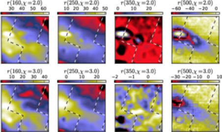
Figure 7: The fit residuals for models with the OH dust and the radiation field intensity scaled by factors $\chi$=2 and 3. The values are relative errors $I_{\rm Obs}-I_{\rm Mod}$ in per cents of the observed surface brightness $I_{\rm Obs}$. The area is this and the subsequent plots of model results is $10\arcmin\times 10\arcmin$ and the plots are centred at coordinates $\alpha_{\rm 2000}$=19^h0^m54.3^s, $\delta_{\rm 2000}$=-36$\degr$55$\arcmin$22$\arcsec$.

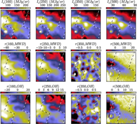
Figure 8: A model fit to the Herschel surface brightness data with an isotropic radiation field four times the ISRF of Mathis et al. (1983). The first row shows the original observations. The other rows show the errors, ($I_{\rm Obs}-I_{\rm Mod}$)/$I_{\rm Obs}$, in units of per cent. The second row corresponds to the MWD dust model (Draine 2003), and the bottom row to the OH dust model (Ossenkopf & Henning 1994). To exclude the regions affected by boundary effects, each frame shows the central $8.3\arcmin\times 8.3\arcmin$ area of the whole model that covered an area of $10\arcmin\times 10\arcmin$. To guide the eye, the dashed lines show the outline of the area covered by the NIR observations.

More satisfactory solutions are found by scaling the ISRF values by a factor of $\chi=$4. Figure 8 shows the observed surface brightness maps and the fit residuals for both the MWD and OH dust models. Because the model is fitted only based on the 350 $\mu$m intensity, and the product of the radiation field and column density is capable of producing high enough surface brightness, the rms error at this wavelength is now below 1%.

Concentrating on the central area, the fit is better with the OH model. Apart from the noise affecting the low column density part, the relative errors are $\sim$10% at both 250 $\mu$m and 500 $\mu$m. There is no strong overall bias even at 160 $\mu$m. This indicates that the average shape of the SED is well reproduced. There are, however, some systematic effects. The observed level of the 500 $\mu$m emission is well reproduced in the filament but is overestimated is the lower density regions. The error is small, $\sim$10%, and could be associated with the uncertainty of the intensity zero point of the observations. A stronger effect is seen at the location of the eastern clump, near the boundary of the area shown. There the observed 500 $\mu$m surface brightness is up to $\sim$15% lower than the model prediction. The percentage error is not large but it is very clear in the map and significant considering that the nearby wavelength of 350 $\mu$m is perfectly fitted. In the same area the model fails to produce sufficiently high surface brightness at short wavelengths, the error increasing to $\sim$30% at 160 $\mu$m. One possible interpretation is that the actual radiation field is higher in this area. By underestimating the heating, the model would require a column density that is too high to explain the 350 $\mu$m map (hence the high 500 $\mu$m signal) but does not include enough warm dust to reproduce the shorter wavelengths. The 160 $\mu$m (and 250 $\mu$m) residuals show a general gradient towards south-east that can indicate an increase of the radiation field intensity. This would be consistent with the higher level of NIR scattered light seen in that direction (see Sect. 3.2). An alternative explanation for the behaviour of the eastern clump involves the dust opacity spectral index. A higher $\beta$ value might be needed to correct the ratio between the 350 $\mu$m and 500 $\mu$m data that are relatively insensitive to variations in the dust temperature.

The error maps of the MWD model look qualitatively similar to the OH results but the $\chi^{2}$ value (considering maps other than the 350 $\mu$m) is worse by more than a factor of two. Outside the filament the 160 $\mu$m and the 250 $\mu$m signals are mainly overestimated and thus the emission appears too warm. However, the 250–500 $\mu$m spectral index of MWD is 2.1, i.e., higher than the value $\beta$=1.76 of the OH model.Therefore, compared to the OH dust model, the best fit would also be expected to correspond to a somewhat lower value of the radiation field. In the eastern clump the 500 $\mu$m emission is again overestimated and the $160\,\mu$m emission underestimated but, possibly because of the different $\beta$ values, the errors are smaller. There is still a gradient towards south-east consistent with an increase in of the dust temperature. However, as already noted, the sign of the 160 $\mu$m errors has changed compared to the OH model, and the MWD model would produce insufficient intensity at the southern side of the filament.

We show in Fig. 9 the $A_{\rm V}$ map and the filament profile for the OH model where the Mathis et al. (1983) radiation field was scaled by a factor of four. Because of the isotropy of the radiation field, the shape of the recovered profile is similar to that of $A_{\rm V}^{\rm sub-mm}$. However, the predicted $A_{\rm V}$ values are not just higher than the previous $A_{\rm V}^{\rm sub-mm}$ estimates, which is possible for a number of reasons, but also higher than the measurements of $A_{\rm V}^{\rm NICER}$. This is an indication that either the assumption of the NIR extinction curve (used in the conversion of NIR colour excesses to $A_{\rm V}$) is incorrect or, more likely, the ratio $\tau(0.55\,\mu{\rm m})/\tau(350\,\mu{\rm m})$ used in the modelling is incorrect. An increase in the sub-millimetre opacity would decrease the model $A_{\rm V}$. If this modification were restricted to the centre of the filament, the radiation field would not have to be changed and the correct shape of the SED would still be recovered at low and intermediate column densities. In the same figure we also show again the minimum and maximum $A_{\rm V}^{\rm NICER}$ profiles along the selected stripe (dotted lines). The shape and magnitude of $A_{\rm V}^{\rm sub-mm}$ in again seen to be in agreement with the maximum $A_{\rm V}^{\rm NICER}$ profile rather than the average profile.

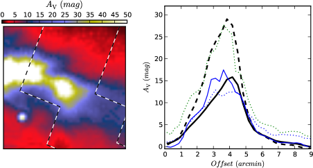
Figure 9: The visual extinction in the model with OH dust and an isotropic radiation field with the intensity four times the standard value (Mathis et al. 1983). The left hand frame shows the $A_{\rm V}$ map from the model smoothed to a resolution of 18$\arcsec$. The right hand frame shows the $A_{\rm V}$ profile of the model (dashed line) compared to the observed profiles of $A_{\rm V}^{\rm sub-mm}$ (thick solid line) and $A_{\rm V}^{\rm NICER}$ (thin blue line) along the selected stripe. The latter two are the same as in Fig. 5b but are shown at their original resolution. In the plot the $A_{\rm V}^{\rm sub-mm}$ has been scaled by a factor of 1.3. The dotted lines are the profiles of the maximum and minimum $A_{\rm V}^{\rm NICER}$ along the stripe.

The previous study of the NIR observations and Spitzer FIR data suggested an anisotropy with a stronger radiation field in the south (Juvela et al. 2009). Figure 5 lead to a similar conclusion. Because the Galactic plane is located north of Corona Australis cloud, there must be a more local cause for the asymmetry. The star S CrA is located on the south side of the filament, immediately east of the area covered by our NIR data. The Herbig Ae/Be star R Corona Australis is farther in the east (Gray et al. 2003). The stars appear to affect the dust emission at least in the eastern part of our maps (as seen in Fig. 7). The precise spectral type of S CrA is not known (the main component S CrA A was classified as G5Ve by Carmona et al. (2007)). Based on the observed K band magnitude of S CrA, $m_{\rm K}=6.1^{\rm m}$, the NIR intensity produced by S CrA is comparable to the general ISRF up to distances corresponding to several arc minutes. R CrA may have similar contribution to the NIR radiation field although, because of large intervening extinction, its effect on dust heating is probably smaller. The other bright stars in the region, HD 176269 and HD 176270, are near the south end of the area covered by our NIR observations (see Fig. 2). The distance estimates of these B9V stars are uncertain but they may both be associated with the cloud (see Peterson et al. 2011).

We examine the situation by illuminating the model cloud with an isotropic ISRF component and adding a second radiation source in the southern direction, at a position angle of 20 degrees from south to east. The source is assumed to be at a large distance. Both radiation field components are assumed to have the same spectral shape as the normal ISRF and their combined energy input is kept the same as in Fig. 9, four times that of the normal ISRF.

When the southern source stands for 25% of the total radiation field energy, the north-south gradients in the residuals of the 160 $\mu$m and 500 $\mu$m fits disappear (Fig. 10). Thus the north-south radiation field anisotropy is now correct as far as can be concluded from the FIR and sub-mm emission. The result assumes that the additional radiation is coming directly from the SE direction. If the direction for the incoming radiation is not perpendicular to the line-of-sight (e.g., more on the front side of the cloud), the actual anisotropy of the radiation field may be larger. Because the dust is now warmer on the southern side of the filament the maximum of the column density should move towards north thus increasing the discrepancy with $A_{\rm V}^{\rm NICER}$ that peaks south of $A_{\rm V}^{\rm sub-mm}$. However, as shown in Fig. 11, the effect on the shape of the model column density profile is not significant. The gradient in the east-west direction still remains unexplained by the model. More specifically, the clump near the east boundary of the NIR map shows, compared to our model, an excess at 250 $\mu$m and low surface brightness at 500 $\mu$m. As already noted, this can be a sign of a further temperature gradient (natural considering the vicinity of the R CrA region) possibly combined with an increase in the dust spectral index.

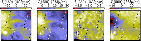
Figure 10: The relative errors (%) in the predicted surface brightness in the case of an anisotropic radiation field and the OH dust model.

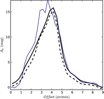
Figure 11: The $A_{\rm V}$ profile of the filament as determined from the radiative transfer model with an anisotropic radiation field (dashed lines, scaled with 0.5). The profile is compared with the $A_{\rm V}^{\rm NICER}$ (blue solid line) and the $A_{\rm V}^{\rm sub-mm}$ profile (solid black line, scaled with 1.3).

If the ISRF level is further increased by 20%, the column densities decrease but the $\chi^{2}$ values are higher by more than a factor of two, mainly because the 160 $\mu$m intensities are overestimated throughout the field. This indicates that, apart from the inherent uncertainties involved in the modelling, the total intensity of the radiation field is well constrained. The models cannot produce sufficient surface brightness with lower level of heating and with increased ISRF the spectrum becomes incorrect. However, if the dust opacity in the cloud centre increases by a factor of a few, the lower limit of the ISRF could be relaxed correspondingly.

4.2 Modelling of the NIR scattered light

We calculate the NIR surface brightness maps for the previous models where the radiation field corresponded to four times the normal ISRF (Mathis et al. 1983) and the field is either isotropic or anisotropic. In the models of the sub-millimetre dust emission, the density distributions are similar for the MWD and the OH dust, the column densities being only $\sim 20$% higher for the MWD. Therefore, in the following we consider only the density distributions derived from the fits of the Herschel data with the OH dust model. With this fixed density distribution, the scattered light can be calculated using both the MWD and the OH dusts. The OH model does not specify the scattering function (i.e., the directional distribution of scattered photons) and we use the same scattering function as in the case of MWD.

The differences between the optical and near-infrared properties of the two dust models are important as can be seen in Fig. 12. For MWD the scattering is still dominant in the $J$ band while for the OH model the efficiencies $Q_{\rm Sca}$ and $Q_{\rm Abs}$ are almost equal. In $J$ band the albedos are 0.68 and 0.58 for MWD and OH, respectively. In case of multiple scattering, the effect on the surface brightness can be expected to be noticeable.

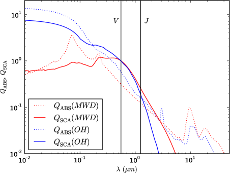
Figure 12: The scattering and absorption efficiencies for the two dust models. The solid curves show the scattering efficiencies $Q_{\rm Sca}$ for the MWD dust (solid red line) and the OH dust (solid blue line) that have been normalised to a value of 1.0 in the $V$ band (0.55 $\mu$m). The dotted lines are the corresponding efficiencies for absorption, $Q_{\rm Abs}$, that have been scaled with the same factors as the $Q_{\rm Sca}$ values.

The surface brightness images are shown in Fig. 13. For the MWD dust, the predicted surface brightness levels are of the right order of magnitude. The $H$ band levels are very close to the right value, the $J$ band values are $\sim$30% higher than the observed values and the $K$ band values are lower by a similar amount. This could point to a NIR spectrum of the ISRF that is redder than in the Mathis et al. (1983) model. Juvela et al. (2008) obtained similar results noting that in particular the $H$ and $K$ band values were twice as high as expected in the case of the normal ISRF. In the present study, the modelling also takes into account the effect that the optically thick filament has on the radiation field. This shadowing is probably the main reason why the modelling prefers higher values for the intensity of the external radiation field.

The NIR calculations fail to reproduce the surface brightness dip that is evident in the observations. If the modelling of the dust emission underestimates the column density at the centre of the filament, this could also partly explain the difference in the NIR colours. Because the NIR scattering takes place is mostly in the forward direction, an increase in the column density would make the spectrum of the scattered light redder. Higher column densities would appear to be incompatible with the $A_{\rm V}^{\rm NICER}$ data but, because no stars are seen through the centre of the filament (see Fig. 7 in Juvela et al. 2008), this cannot be excluded on the basis of $A_{\rm V}^{\rm NICER}$ alone. The present model is based on the modelling of dust emission and already has a peak extinction that is twice the maximum of the $A_{\rm V}^{\rm NICER}$ map. If the radiation field intensity is decreased by a factor of two, the column density could increase almost without limit and there would be no constraints on the maximum column density. This is excluded only by the fact that a lower intensity of the radiation field would alter the SED of the dust emission in a way that is incompatible with the observations.

The OH dust model (Fig. 13, bottom row) reproduces the morphology of the NIR data better than the MWD dust model. The dip in the $J$ band is now noticeable at the location of the dense clump. The depth of the depression is about half of the peak values around the central clump. This is still far from the almost complete absence of scattered light in the observations but is clearly a step in the right direction. A small depression is seen even in the $Ks$ band where the MWD dust produced a clear peak. The maximum $J$ band intensity is again slightly higher than the observed values. On the other hand, the $Ks$ band signal is very low, only one quarter of the observed.

We show in Fig. 14 similar calculations for the model of Fig. 10. The scattered light is calculated consistently assuming that, in addition to an isotropic radiation field component, 25% of the total radiation comes from the southern direction. The resulting surface brightness asymmetry between the south and north side of the filament is already slightly too large. Although the ratio of 3:1 between the isotropic and the anisotropic radiation field components was appropriate for the distribution of dust emission, the NIR surface brightness at least precludes larger degree of anisotropy, assuming that the spectrum of the anisotropic source is the same as for the isotropic component.

The major shortcoming of the models is the absence of a sufficiently strong surface brightness dip at the location of the main clump. This could be caused either by the column densities being underestimated (unlikely given the extinction data) or by some modification of the dust properties. To check the first alternative and to check that the previous differences between the OH and MWD models were not just the effect of different opacities (instead of the albedo), we recalculated the MWD model after scaling its densities by a factor of two. This results only a very minor improvement (see Fig. 15) although the maximum of the $A_{\rm V}$ map is already well over $100^{\rm m}$. The effect on the morphology of the NIR maps is smaller than the difference between the two dust models.

The models predict higher 870 $\mu$m intensities than those observed with LABOCA (see Fig. 16). However, a large fraction of the difference can be explained by the spatial filtering that removes large scale structure from the LABOCA map. In the NIR observations the $J$ band surface brightness goes almost to zero at the centre of the main clump. This is difficult to explain because some scattered light is always observed from the outer cloud layers. Thus, the explanation may require a very special geometry (e.g., a smaller line-of-sight extent of the cloud at the location of the clump) and/or further modifications to the dust models as suggested by the difference between the MWD and OH model results. Although the NIR signal saturates by $A_{\rm V}\sim 20^{\rm m}$, the data still set very strong constraints both on the cloud structure and the dust properties.

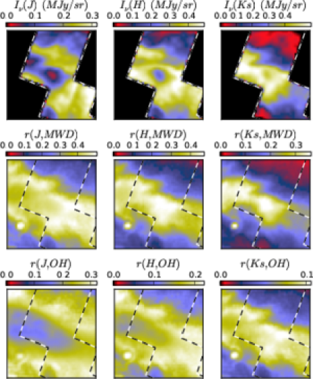
Figure 13: The observed NIR surface brightness (first row) and the surface brightness predicted for the models based on the Herschel sub-millimetre data (OH dust, $\chi=$4.0). The second and the third rows correspond to calculations of the scattered light with the MWD and the OH dust models, respectively, in case of isotropic illumination.

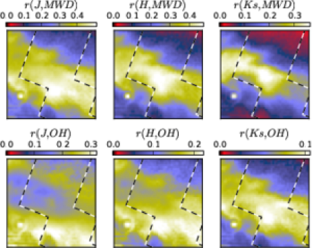
Figure 14: The NIR surface brightness for the models with anisotropic radiation field. The first and the second row correspond to calculations of the scattered light with the MWD and the OH dust models, respectively.

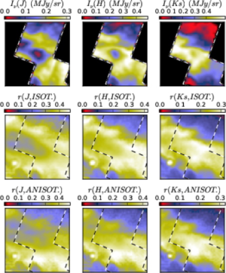
Figure 15: The observed NIR surface brightness (first row) and the surface brightness predicted by models with the densities twice the values of those fitting the sub-millimetre data. The second and the third row correspond to the cases of isotropic and anisotropic radiation field, respectively.

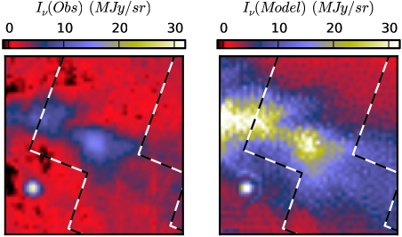
Figure 16: Comparison of the observed 870 $\mu$m surface brightness and the prediction from the model with $\chi=4.0$ with the OH dust.

4.3 Sensitivity to the cloud shape

In the modelling the column density structure is determined directly by the observations. For fixed dust properties and a fixed external radiation field the result should be unique. However, there are still factors connected with the density distribution that can affect the results. The actual three-dimensional shape of the cloud is unknown. Although the morphology suggests the presence of a single cylindrical filament, the cloud could still be flattened or elongated along the line-of-sight. Some effects can also result from small scale inhomogeneities that allow short wavelength radiation to penetrate deeper into the cloud. We tested the sensitivity of the results to these factors using the model presented in Fig. 10.

The clumpiness was implemented by multiplying the density of each cell in the model by a random number uniformly distributed between zero and one. This results in a fair amount of inhomogeneity considering that the cloud radius is only $\sim$30 cells. All densities were then rescaled so that the model again reproduced the observed 350 $\mu$m surface brightness. Compared to the original model with a smooth density distribution, this resulted in less than 10% changes in the column density along individual lines-of-sight. More importantly, this level of inhomogeneity did not introduce significant systematic change in the column density nor in the intensity of NIR scattered light produced. Of course, the effects would be stronger if the cloud included large continuous cavities extending to the centre of the cloud.

The overall cloud shape was varied by changing the FWHM of the line-of-sight density distribution by $\pm$30%. The column densities were again adjusted according to the 350 $\mu$m data. When the cloud was 30% more extended along the line-of-sight, the resulting column density towards the model centre was lower by $\sim$20%. When the cloud was flattened by 30%, the percentual increase of the model column density was closer to 40%. These numbers do not yet take into account the fact that a for the best fit to the observed SED also the intensity of the external radiation field might have to be readjusted. This could reduce the net change of the column density. However, with the radiation field of Fig. 10 the 160 $\mu$m surface brightness was already correct to within $\sim$10%.

We conclude that the uncertainty of the three-dimensional shape of the cloud translates to an uncertainty of some tens of per cent in the column density. These uncertainties affect the accuracy to which the dust opacity can be determined. However, the modelling is better constrained when independent extinction measurements are available.

5 Conclusions

We have examined the structure of the northern filament of the Corona Australis cloud using the combination of Herschel sub-millimetre data and near-infrared observations. The study has lead to the following conclusions:

• At $A_{\rm V}<15^{\rm m}$ the three column density estimators, the thermal dust emission, the NIR reddening of the background stars, and the surface brightness caused by the NIR scattered light, are all linearly related to each other. The differences in the actual numbers can be explained by the uncertainty of the dust opacity and of the radiation field intensity.

• At low column densities ($A_{\rm V}\sim 10^{\rm m}$ or below) the scattered light provides the best column density map in terms of resolution. Its predictions are very tightly correlated with the estimates obtained from the dust emission. However, the slope of the relation depends on the intensity of the radiation field.

• Based on the dust emission, the north-south column density profile was observed to be skewed with a sharp drop in the column density on the northern side. The profile obtained from the reddening of the background stars is more symmetric but is strongly affected by the lack of stars visible through the central filament.

• The modelling of the dust emission suggests that the radiation field intensity at the location of the cloud filament is about four times the value of the normal ISRF. The value can be lowered only by assuming that the dust sub-millimetre opacity has increased at the centre of the filament. However, the models of the NIR scattered light are also consistent with an elevated radiation field intensity.

• According to the models, the radiation field is anisotropic with an approximate ratio of 3:1 between the isotropic component and additional radiation coming from the southern direction.

• The models are unable to reproduce the deep dip in the NIR surface brightness at the centre of the filament. One possible explanation is a change in the dust properties (as indicated by the differences between the dust models examined) that has lowered the NIR albedo.