Molecular Outflows Identified in the FCRAO CO Survey of the Taurus Molecular Cloud

Abstract

Jets and outflows are an integral part of the star formation process. While there are many detailed studies of molecular outflows towards individual star-forming sites, few studies have surveyed an entire star-forming molecular cloud for this phenomenon. The 100 square degree FCRAO CO survey of the Taurus molecular cloud provides an excellent opportunity to undertake an unbiased survey of a large, nearby, molecular cloud complex for molecular outflow activity. Our study provides information on the extent, energetics and frequency of outflows in this region, which are then used to assess the impact of outflows on the parent molecular cloud. The search identified 20 outflows in the Taurus region, 8 of which were previously unknown. Both ¹²CO and ¹³CO data cubes from the Taurus molecular map were used, and dynamical properties of the outflows are derived. Even for previously known outflows, our large-scale maps indicate that many of the outflows are much larger than previously suspected, with eight of the flows (40%) being more than a parsec long. The mass, momentum and kinetic energy from the 20 outflows are compared to the repository of turbulent energy in Taurus. Comparing the energy deposition rate from outflows to the dissipation rate of turbulence, we conclude that outflows by themselves cannot sustain the observed turbulence seen in the entire cloud. However, when the impact of outflows is studied in selected regions of Taurus, it is seen that locally, outflows can provide a significant source of turbulence and feedback. The L1551 dark cloud which is just south of the main Taurus complex was not covered by this survey, but the outflows in L1551 have much higher energies compared to the outflows in the main Taurus cloud. In the L1551 cloud, outflows can not only account for the turbulent energy present, but are probably also disrupting their parent cloud. We conclude that for a molecular cloud like Taurus, a L1551-like episode occuring once every $10^{5}$ years is sufficient to sustain the turbulence observed. Five of the eight newly discovered outflows have no known associated stellar source, indicating that they may be embedded Class 0 sources. In Taurus, 30% of Class I sources and 12% of Flat spectrum sources from the Spitzer YSO catalogue have outflows, while 75% of known Class 0 objects have outflows. Overall, the paucity of outflows in Taurus compared to the embedded population of Class I and Flat Spectrum YSOs indicate that molecular outflows are a short-lived stage marking the youngest phase of protostellar life. The current generation of outflows in Taurus highlights an ongoing period of active star-formation, while a large fraction of YSOs in Taurus has evolved well past the Class I stage.

1 Introduction

From the emergence of a hydrostatic core, the collapse of a proto-stellar core is accompanied by winds and mass loss (Lada, 1985) probably driven by magnetospheric accretion (eg. Koenigl, 1991; Edwards et al., 1994; Hartmann et al., 1994). Integrated over time, the effect of a wind from a young star is to blow away the placental material left over from its birth and which shrouds it during its earliest evolution. The discovery of bipolar molecular outflows has been a key to the understanding of this process (eg. Snell et al., 1980). These molecular outflows have dimensions of up to several parsecs, masses comparable or more than than their driving sources, and tremendous kinetic energies, typically 10⁴⁵ ergs (Bally & Lada, 1983; Snell, 1987). Such massive flows must represent swept-up material as the winds, emerging from the star and/or its circumstellar disk, interact with their ambient medium.

While jets and outflows are an integral part of the star formation process, only a few studies out of the many detailed studies of molecular outflows towards individual star-forming sites, have a molecular cloud-wide view of this phenomenon. One of these is the recent study of outflows in Perseus (Arce et al., 2010). The Taurus molecular cloud with its proximity (140 pc) and displacement from the Galactic Plane (b$\sim-19^{\circ}$) affords high spatial resolution views of an entire star forming region with little or no confusion from background stars and gas. The most complete inventory of the molecular gas content within the Taurus cloud is provided by Ungerechts & Thaddeus (1987), who observed ¹²CO J=1-0 emission from 750 deg² of the Taurus-Auriga-Perseus regions. They estimate the molecular mass resident within the Taurus-Auriga cloud to be $3.5\times 10^{4}$ M_⊙. However, the $30^{\prime}$ angular resolution of this survey precludes an examination of the small scale structure of the cloud. The recently completed 100 square degree FCRAO CO survey with an angular resolution of 45^′′, sampled on a 20^′′ grid, and covered in ¹²CO and ¹³CO simultaneously, reveals a very complex, highly structured cloud morphology with an overall mass of $2.4\times 10^{4}$ M_⊙ (Narayanan et al., 2008; Goldsmith et al., 2008). This survey provides an excellent opportunity to perform an unbiased survey of a large, nearby, molecular cloud complex for molecular outflow activity. Goldsmith et al. (2008) divide the Taurus cloud into eight regions of high column density that include the L1495, B213, L1521, Heiles Cloud 2, L1498, L1506, B18, and L1536, and tabulate the masses and areas of these well-known regions. Of these, the L1495 and B213 clouds have been recently studied using JCMT HARP ¹²CO J=3-2 observations, searching for molecular outflows from young stars (Davis et al., 2010a), where they have detected as many as 16 outflows.

Targeted studies with higher angular resolution of ¹³CO and C¹⁸O emission from individual sub-clouds of Taurus reveal some of the relationships between the molecular gas, magnetic fields, and star formation but offer little insight to the coupling of these structures to larger scales and features, nor do they provide an unbiased search for molecular outflows (Schloerb & Snell, 1984; Heyer et al., 1987; Mizuno et al., 1995; Onishi et al., 1996). A list of $\sim 300$ Young Stellar Objects (YSOs) derived from multi-wavelength observations have been compiled by Kenyon & Hartmann (1995), and this list was compared to the column density distribution of molecular gas by Goldsmith et al. (2008). This list of young stars has been recently complemented by observations from the Spitzer Space Telescope (Rebull et al., 2010; Luhman et al., 2010). A comprehensive review of the entire Taurus region is provided by Kenyon et al. (2008). In this paper, we use the up-to-date list of young stars from the Spitzer observations, and the list from Kenyon et al. (2008). A list of Molecular Hydrogen emission-line Objects (MHOs) that includes the Taurus region has also been recently compiled (Davis et al., 2010b), and this list is also compared against our data in this paper.

It should be noted that the FCRAO Taurus Molecular Cloud survey has an overall rms uncertainty (in T${}_{A}^{*}$ K units) of $\sim 0.58$ K and $\sim 0.26$ K in in ¹²CO and ¹³CO transitions respectively (Narayanan et al., 2008). Detecting all outflow sources in Taurus was never a goal of this survey, nevertheless, the rms sensitivity levels reached is indeed lower than the original goals of the project, and this allows us to use this survey to probe for outflows. In this paper, we provide an unbiased search for outflows in the FCRAO Taurus survey, identify their driving sources, evaluate outflow properties, and compare these properties with those of the driving sources, and associated molecular cloud environments. The structure of this paper is as follows. In §2.1, we summarise the observations and describe our data processing and analysis with respect to the search criteria to detect outflows, and subsequent analysis of their properties. In §3, we summarise the main results, and tabulate the properties of the detected outflows. In §4, we compare the outflows against the energetics of the driving sources, and the cloud environment. In §5, we summarise our results.

2 Observations and Data Processing

2.1 Observations

Details of the observations, data collection and data processing steps of the original Taurus Molecular Cloud survey are presented in Narayanan et al. (2008). Here, for completeness, we describe the salient details of the dataset. The observations were taken with the 14 meter diameter millimetre-wavelength telescope and the 32 pixel focal plane array SEQUOIA (Erickson et al., 1999) of the Five College Radio Astronomy Observatory. The FWHM beam sizes of the telescope at the observed frequencies are 45″ (115.271202 GHz) and 47″ (110.201353 GHz). The main beam efficiencies at these frequencies are 0.45 and 0.50 respectively as determined from measurements of Jupiter. Previous measurements of the extended error beam of the telescope and radome structure were performed by measuring the disks of the sun and moon, and indicate that there can be $\sim 25$% net contribution from extended emission outside the main beam from a region $\sim 0.5\mbox{${}^{\circ}$}$ in diameter. The shape of this error beam is approximately circular, but the amount of contribution of emission at any given point from this error beam pattern depends on details of the distribution of the emission from the source, however this contribution is expected to be negligible for outflows. All data presented here are in T${}_{A}^{*}$ (K), uncorrected for telescope beam efficiencies. The backends were comprised of a system of 64 auto-correlation spectrometers each configured with 25 MHz bandwidth and 1024 spectral channels. No smoothing was applied to the auto-correlation function so the spectral resolution was 29.5 kHz per channel corresponding to 0.076 km s^-1 (¹²CO) and 0.080 km s^-1(¹³CO) at the observed frequencies. The total coverage in velocity is 65 km s^-1 (¹²CO) and 68 km s^-1 (¹³CO) respectively. The spectrometers were centred at a v_LSR of 6 km s^-1.

The Taurus Molecular Cloud was observed over two observing seasons starting in November 2003 and ending in May 2005. The ¹²CO and ¹³CO lines were observed simultaneously enabling excellent positional registration and calibration. System temperatures ranged from 350-500 K for the ¹²CO line and 150-300 K for the ¹³CO line.

2.2 Previously Known Outflows and YSOs in Taurus

The list of outflows compiled by Wu et al. (2004) contains 13 outflows in the area covered by the FCRAO Taurus survey. In addition, we found three previously identified outflows that were missed by Wu et al. (2004). Two of these outflows (IRAS 04169+2702 and IRAS 04302+2247) were from the survey of Bontemps et al. (1996). The other outflow (IRAS 04240+2559) was discovered by Mitchell et al. (1994) and is associated with DG Tau. Thus the number of previously known outflows candidates is 16, and these are given in Table 1. In the last column of this table we describe the nature of the outflow, whether bipolar or with only red or blue outflow, and give appropriate references.

Recently, Davis et al. (2010a) surveyed an approximately one square degree region of the L1495 region of Taurus in the CO J=3-2 line using HARP on the JCMT. They identify as many as 16 molecular outflow candidates in this region. They confirm the detection of several well-known outflows and several of their outflows we believe are part of much larger outflows that will be discussed later. We note that many of their outflow candidates are identified based on wing emission at relatively low-velocities (2.5 km s^-1) from the ambient cloud line centre velocity. The velocity field in Taurus is very complex, which can be seen in the channel maps presented in Narayanan et al. (2008), and often there are secondary velocity components that might mimic outflows. Thus the identification of outflows based on a simple formula without examining the large-scale environment can be fraught with difficulties. We have not included the results of Davis et al. (2010a) in Table 1, but instead, we have integrated their results into the discussion in our Results section.

Based on observations of mid and far-infrared bands with the Spitzer Space Telescope, Rebull et al. (2010) tabulate the properties of pre-main-sequence objects in Taurus. Their survey covers $\sim 44$ deg², and encompasses most of the highest column density regions of the Narayanan et al. (2008) study. This Spitzer Survey lists 215 previously known members in Taurus, and they identify and tabulate properties of 148 new candidate members. All 363 of these YSOs are over-plotted in applicable areas in the plots presented below, with the previously known candidates plotted as red stars, and new candidate members as red triangles.

We also use the data from the General Catalogue of Herbig-Haro (HH) objects, 2nd edition compiled by Bo Reipurth. In addition, we plot the molecular hydrogen emission-line objects (the so-called MHOs), which are the shock-excited IR counterparts to the HH objects from the list compiled by Davis et al. (2010b).

Table 1: List of Known Outflows in Taurus

Names	RA (J2000)	Dec (J2000)	Comments
IRAS04166+2706	04:19:42.6	27:13:38	Bipolara,b
IRAS04169+2702	04:19:58.4	27:09:57	Bipolara
IRAS04181+2655 (CFHT-19)	04:21:10.53	27:02:06.0	Bipolara
IRAS04239+2436	04:26:56.9	24:43:36	Red Lobe, HH300 flowc
IRAS04240+2559 (DG Tau)	04:27:04.7	26:06:17	Red lobe, optical jetd
IRAS04263+2426 (Haro 6-10)	04:29:23.7	24:32:58	Bipolar flowe
IRAS04278+2435 (ZZ Tau)	04:30:53.0	24:41:40	Red Lobef
TMC 2A	04:31:59.9	24:30:49	bipolar g
L1529	04:32:44.7	24:23:13	not confirmedh,i
IRAS04302+2247	04:33:16.8	22:53:20	bipolara
IRAS04325+2402 (L1535)	04:35:33.5	24:08:15	Redf
IRAS04361+2547	04:39:13.9	25:53:21	Bipolara,j
IRAS04365+2535 (TMC1A)	04:39:34.8	25:41:46	Bipolara,k,l
IRAS04368+2557 (L1527)	04:39:53.3	26:03:06	Bipolara,l,m,n
IRAS04369+2539 (IC 2087)	04:39:58.9	25:45:06	Redf
IRAS04381+2540 (TMC1)	04:41:13.0	25:46:37	Bipolara,k

a) Bontemps et al. (1996); (b) Tafalla et al. (2004); (c) Arce & Goodman (2001); (d) Mitchell et al. (1994); (e) Stojimirović et al. (2007); (f) Heyer et al. (1987); (g) A complicated region mapped by Jiang et al. (2002) with a likely bipolar outflow associated with 04292+2422 (Haro 6-13) and possible a second outflow associated with 04288+2417 (HK Tau); (h) Lichten (1982); (i) Goldsmith et al. (1984); 04292+2422 Haro 6-13; (j) Terebey et al. (1990); (k) Chandler et al. (1996); (l) Tamura et al. (1996); (m) Hogerheijde et al. (1998); (n) Zhou et al. (1996).

2.3 Data Processing

For all the details of the data processing of the original Taurus survey, refer to Narayanan et al. (2008). In this paper, we start with the 88 ’hard-edge’ cubes covering the full $100$ square degrees. The 88 hard-edge cubes form a grid of $11\times 8$ data cubes. They are dubbed hard–edge cubes, as they do not have overlapping regions between two contiguous cubes. Each ’hard-edge’ cube is assembled from a set of input regridded $30\arcmin\times 30\arcmin$ cubes, after removing the spectral and spatially derived baselines described above from each cube, and subsequently averaging the data together, weighting them by $\sigma^{-2}$, where $\sigma$ is the rms in the derived baseline. In angular offsets, the full extent of the combined hard–edge cubes are (5.75^∘, $-5.75$^∘) in RA offsets and ($-2.75$^∘, 5.75^∘) in Dec offsets from the fiducial centre of the map ($\alpha$(2000) = $04^{h}32^{m}44.6^{s}$, $\delta$(2000) = $24\mbox{${}^{\circ}$}25\arcmin 13.08\arcsec$). Thus for the full $11.5\mbox{${}^{\circ}$}\times 8.5\mbox{${}^{\circ}$}$ region spaced at 20″, there are 3,167,100 spectra in each isotopologue in the combined set of hard–edge cubes. Most of the hard–edge cubes have a spatial size of 1 square degree, except for the cubes that lie on the four edges of the region covered, which measure 1.25 square degrees. The hard–edge cubes at the four corners of the Taurus map have a size of 1.5625 square degrees ($1.25\mbox{${}^{\circ}$}\times 1.25\mbox{${}^{\circ}$}$).

2.3.1 Unbiased Search for Outflows

Our unbiased search for outflows from the Taurus Molecular Cloud Survey was carried out as follows. The systemic velocity of most of the Taurus emission (from the ¹³CO data) varies from $\sim$ 6 to 7 km s^-1. So we initially define outflow wings to be at least 3 km s^-1 offset from the systemic velocity, and define a blueshifted outflow velocity range of $-1$ to $3$ km s^-1, and a redshifted outflow velocity range of $9$ to $13$ km s^-1. We make integrated intensity images of blueshifted and redshifted emission in ¹²CO in the aforementioned velocities in each of the 88 hard-edge cubes, and overlay them both against an integrated intensity image made between the velocities of 4 to 8 km s^-1 in ¹³CO. Due to the lower optical depth of the isotopic transition, the integrated intensity in ¹³CO at low velocities represents the emission from the ambient cloud medium. By overlaying the higher velocity linewing emission from ¹²CO, these plots are meant to reveal the distribution of ambient gas, and highlight the distribution of any high-velocity redshifted and/or blueshifted gas that may be present. Many such examples of these kind of plots will be presented below. When we see any extended blueshifted or redshifted linewing emission, for any hard edge cube, we follow it up with other tests to ascertain the presence of outflows.

In addition to the 88 hard-edged cubes, we have 88 rms images each in ¹²CO and ¹³CO, where these images are derived from evaluating the rms noise level in spectral windows where no line emission is present. Propagating errors, it is thus possible to obtain integrated intensity images along with the corresponding uncertainties at every pixel location in a map. When extended high-velocity features are seen, we compute average spectra over these regions. To isolate emission from the presumed outflow lobes, polygonal areas delineating the presumed outflow lobes are interactively drawn, and our procedure then obtains average ¹²CO and ¹³CO spectra within these polygonal regions. However, the presence of significant emission in the previously defined blueshifted and redshifted velocity intervals is not a sufficient requirement to identify outflows. The velocity structure of the Taurus Molecular Cloud is complex, and in many regions there are additional cloud components that appear in these velocity intervals which are used to identify outflows. To distinguish between outflows and secondary velocity components, we made use of our large maps, and the emission in both isotopic species. Extended narrow-line features seen in both ¹²CO and ¹³CO  although in the velocity interval defined as outflow emission, are almost certainly secondary cloud components and not outflows. We have applied a relatively strict set of criteria in identifying outflow, thus we believe that the outflows in our final list are in fact true outflows.

When extended blueshifted or redshifted regions of emission are seen, we follow that by constructing position-velocity (PV) diagrams that cut through these regions. The PV cuts are chosen to cut through the bulk of the redshifted and/or blueshifted emission, and where available, passing through the YSO that could be the potential driving source. In these diagrams, outflows usually show up as horizontal or oblique linear features. Examples of these PV diagrams will be shown below. Unassociated foreground or background turbulent cloud components usually show up as vertical features in PV diagram often offset from the low-velocity ambient cloud emission of the bulk material of the Taurus Molecular Cloud.

Overlaid on these integrated intensity images, we can plot the Spitzer sources (Rebull et al., 2010), HH objects, MHO objects (Davis et al., 2010b), previously identified outflow sources in Taurus (Table 1), and the newly identified outflow locations from the JCMT HARP survey (Davis et al., 2010a). In the presence of outflows, the locations of the YSOs and other signposts of star-formation help identify the driving sources for the outflows.

The analyses described in this paper were all performed entirely in python. The hard-edged cubes were manipulated using PyFITS. Plots were made by heavily extending the FITSFigure class provided by APLpy. Astronomical utilities such as coordinate transformations, integrated intensity calculations, position-velocity cuts are all developed in a newly available open-source set of python utilities called idealpy.

3 Results

3.1 List of Detected Outflows

In Figure 1, we present the location of detected outflows overlaid on the molecular hydrogen column density map from Goldsmith et al. (2008). All Taurus YSOs from Spitzer observations are marked in the plot. In addition, the list of hitherto known outflows is denoted in the figure, along with new outflow detections stemming from this study. In Table 2, we present all 20 detected outflows in this study with brief comments on each.

Figure 1: Locations of YSOs and outflow sources in the Taurus Molecular Cloud. The grey scale shows the molecular hydrogen column density map presented in Goldsmith et al. (2008). Red stars show the location of previously known YSOs in Taurus (from Table 4 of Rebull et al. 2010), while red triangles show the location of newly identified YSOs in Taurus (from Spitzer observations and Table 5 of Rebull et al. 2010). Yellow diamonds represent the location of known outflows catalogued in Table 1. Blue squares show the location of previously known outflows identified in this survey, while green circles denote new outflows that have been detected in this current survey.

Figure 2: Overview contour map of blueshifted and redshifted gas about a $78^{\prime}\times 85^{\prime}$ region approximately centred on IC2087, where eight distinct outflows can be seen (individual outflows are called out with arrows). The grey scale shows the ¹³CO integrated intensity map. See Figure 3 for details on symbols and markers. Overlaid on the gray-scale ¹³CO image, ¹²CO blueshifted integrated intensity (within velocity interval -1 to 3.9 km s^-1) is shown in blue dashed contours, and redshifted integrated intensity (8.2 to 13 km s^-1) is shown in red solid contours. Blueshifted contours range from 0.64 to 2.7 in steps of 0.075 K km s^-1, and redshifted contours range from 0.64 to 8.4 in steps of 0.075 K km s^-1.

Table 2: List of detected Outflows

S.No	Name	RA	Dec	New	YSO	Comments
		(J2000)	(J2000)	Detection	Classa
1.	041149+294226	04:11:49.0	29:42:30	Y	–	Bipolar, closely associated
						with new Spitzer source 041159+294236
2.	IRAS04113+2758	04:14:25.2	28:02:21	N	I	Red only
3.	IRAS04166+2706	04:19:42.6	27:13:38	N	I	Bipolar, much longer than
						previously known
4.	IRAS04169+2702	04:19:58.4	27:09:57	N	I	Bipolar
5.	FS TAU B	04:22:00.7	26:57:32	Y	I	Red Lobe only and maybe
						seen in Davis et al. (2010a)
6.	IRAS04239+2436	04:26:56.9	24:43:36	N	I	Red
7.	IRAS04248+2612	04:27:57.7	26:19:19	Y	F	Red Lobe, Optical Flow seen in
						Gomez et al. (1997)
8.	Haro 6-10	04:29:23.7	24:32:58	N	I	Bipolar
9.	ZZ Tau IRS	04:30:53.0	24:41:40	N	F	Red Lobe, first detected by
						Heyer et al. (1987)
10.	Haro 6-13	04:31:50.9	24:24:18	Y	F	Red
11.	IRAS04325+2402	04:35:33.5	24:08:15	N	I	Red
12.	HH 706 flow	04:39:11.4	25:25:16	Y	–	Bipolar
13.	HH 705 flow	04:39:06.7	26:20:29	Y	–	Bipolar
14.	IRAS04361+2547	04:39:13.9	25:53:21	N	I	Bipolar
15.	TMC1A	04:39:34.8	25:41:46	N	I	Blue
16.	L1527	04:39:53.3	26:03:06	N	I	Bipolar
17.	IC2087 IR	04:39:58.9	25:45:06	N	F	Red
18.	TMC-1 North	04:39:59.1	26:19:36	Y	–	Blue
19.	TMC1	04:41:13.0	25:46:37	N	I	Bipolar
20.	045312+265655	04:53:12.1	26:56:55	Y	–	Bipolar

a) From classification of Rebull et al. (2010) when driving source is identified. F indicates Flat spectrum source, which is intermediate between Class I and Class II.

The detected outflows are mostly concentrated in regions of high column density. Individual regions where multiple outflows can be found can be identified in Figure 1. However, the Heiles Cloud 2 region in Taurus is especially notable in that the molecular ring (Schloerb & Snell, 1984) is the seat of many YSOs. In this region, we have detected eight outflows (three of which are new detections; see Figure 2 for an overview figure of this region). More details of the flows in the Heiles Cloud 2 region are presented later in this section.

Below we summarise each outflow in more detail.

3.1.1 041149+294226

In the north-west corner of the region covered in our Taurus survey (see Figure 1), we discover a new bipolar outflow whose driving source is unknown. We call this outflow with the coordinates of the position of a likely origin as 041149+294226. There is a new Spitzer source, 041159+294236 (from Table 4 of Rebull et al. 2010) in the vicinity of this outflow. In Figure 3, which shows a region $\sim 33^{\prime}\times 40^{\prime}$ in size, the blueshifted and redshifted integrated intensity contours of ¹²CO are overlaid on the low-velocity (4 to 8 km s^-1) integrated intensity emission from ¹³CO (shown in greyscale). In this figure, and in all subsequent outflow plots, a variety of symbols representing Spitzer YSOs, HH objects, and outflow sources known in the past are marked when available (see the figure caption of Fig 3 for more details). The outflow has a position angle of $\sim 127^{\circ}$, and appears quite collimated in blueshifted gas, while the redshifted emission is more diffuse. From the tip of the blueshifted lobe to the tip of the redshifted lobe, the full extent of the outflow is 1.6 pc!

The ¹³CO emission shown in Figure 3 is likely tracing the column density of ambient gas representing the cloud core. If so, it appears that the blueshifted gas has broken out of the cloud core, while the redshifted gas from the outflow may be directed into the bulk of the ambient cloud core. The Spitzer source 041159+294236 lies close to the axis of the bipolar outflow and is the only known YSO in this field. However, 041159+294236 is a Class III object, thus as we discuss later, unlikely to be the driving source of this outflow. It is more likely that an hitherto undetected embedded object is the driving source. A position-velocity (p-v) diagram derived along this solid line marked in Figure 3 is shown in Figure 4, where the zero offset position is marked by a yellow dot as the possible location of the driving source in Figure 3. The p-v diagram shows the extended blueshifted line wings due to the outflow but only weak redshifted emission. In Figure 5, we show the average spectra (in both ¹²CO and ¹³CO) obtained towards the regions defined by the red and blue polygons in Figure 3. Broad emission marking the outflow can be seen in the averaged spectra, however the high velocity blueshifted emission is much more prominent than the high velocity redshifted emission. Figures 4 and 5 indicate that the redshifted lobe is not as prominent as the blueshifted one in this source. But, averaged spectra in smaller localized regions of the redshifted lobe do show evidence of redshifted line wings. In general, instead of using just one line of evidence, we use the combination of integrated intensity, position-velocity plots and averaged spectra to identify outflow lobes.

Figure 3: Contour map of blueshifted and redshifted gas around the Spitzer source 041159+294236. The grey scale shows the ¹³CO integrated intensity map. In this and all subsequent outflow maps, the ¹³CO integrated intensity map is always made for a velocity range of 4 to 8 km s^-1(representing the low velocities associated with the ambient cloud emission). In this and all subsequent outflow maps, if present, red stars show the location of previously known YSOs in Taurus (from Table 4 of Rebull et al. 2010), while red triangles show the location of newly identified YSOs in Taurus (from Spitzer observations and Table 5 of Rebull et al. 2010). When available, green hexagons represent locations of known HH objects, and cyan circles represent the locations of claimed outflows from Davis et al. (2010a). Overlaid on the gray-scale ¹³CO image, ¹²CO blueshifted integrated intensity (within velocity interval -1 to 4.2 km s^-1) is shown in blue dashed contours, and redshifted integrated intensity (8.75 to 13 km s^-1) is shown in red solid contours. Blueshifted contours range from 0.45 to 2.2 in steps of 0.075 K km s^-1, and redshifted contours range from 0.5 to 2.3 in steps of 0.075 K km s^-1. In this and other subsequent contour maps, a straight line representing a cut for the position-velocity diagram will be shown followed by a position velocity diagram (for this figure, it is Figure 4), and the yellow circle represents the point representing the origin in the Y-axis of Fig 4. Again, in this figure and all subsequent figures, the blue and red polygons show the regions defined as the blueshifted and redshifted lobes of the outflow, whose average spectra are shown in a figure showing spectra that will follow (for this source, Figure 5).

Figure 4: Position velocity of ¹²CO emission towards 041149+294226 region, through the slice shown in Figure 3 at a position angle of $127^{\circ}$. The contour range is 0.125 to 2.8 K in steps of 0.3 K. Shown in dashed line is the position of the yellow circle shown in Fig 3.

Figure 5: Average Spectra of ¹²CO emission (blue solid lines) and ¹³CO (green dashed lines) towards the blueshifted(left) and redshifted (right) lobes of the outflow in the 041149+294226 region shown in Fig 3. The temperature scale in this and other spectra shown in this paper is in T${}_{A}^{*}$.

3.1.2 IRAS 04113+2758

The first evidence of high velocity gas in this region was provided by Moriarty-Schieven et al. (1992) who surveyed the J=3-2 CO line toward a number of YSOs. Toward IRAS 04113+2758 they detected a CO line with a total velocity extent of 40.3 km s^-1, the largest of any source in their survey. Recently, Davis et al. (2010a) mapped the region with the JCMT as part of the Legacy Survey of the Gould Belt with HARP. Their maps revealed several possible outflows in this regions, including a bipolar outflow with an ill-defined morphology associated with what they call YSO 1/2. We believe YSO 1/2 is coincident with IRAS 04113+2758 (Kenyon et al., 2008).

In Figure 6, we show our map of the redshifted emission in a $\sim 25^{\prime}\times 30^{\prime}$ region about IRAS 04113+2758. The locations of three other possible outflows identified by Davis et al. (2010a) in this region, W-CO-B1, W-CO-flow1 and IRAS 04108+2803A, are denoted by cyan-coloured circles in this figure. The redshifted high velocity emission that we detect is found toward IRAS 04113+2758. The detection of blueshifted emission is complicated by the presence of a second velocity component at V${}_{\rm LSR}\sim$ 4 km s^-1 that is found extending from the south-west corner of Figure 6 to the centre of this Figure. The spectra shown in Figure 9 obtained to the south-east of IRAS 04113+2758 shows this second velocity component in both ¹²CO and ¹³CO emission. Little blueshifted emission is detected blue-ward of the feature as can be seen in Figure 6. We believe that the two blue only outflows (W-CO-B1 and IRAS 04108+2803A) found by Davis et al. (2010a) in this region may be result of the confusion with this widespread secondary velocity component. We note that IRAS 04108+2803 was part of the Moriarty-Schieven et al. (1992) survey, and they detected a relatively narrow line suggesting this is unlikely an outflow source.

The source CW Tau is located north-west of IRAS 04113+2758. This source has a small optical emission-line jet (Gomez de Castro, 1993; Dougados et al., 2000) oriented north-west to south-east. A long slit spectrum (Hirth et al., 1994) found that the south-east jet is blueshifted while the north-west jet is redshifted. Thus, it is very unlikely that CW Tau is the source of the redshifted molecular emission seen in this region.

The p-v diagram shown in Figure 7 shows the high velocity redshifted emission as well as secondary blue velocity component. The averaged spectra within the polygon marked in Figure 8 shows these same features. We note that the spectrum obtained by Moriarty-Schieven et al. (1992) shows very high velocity blue shifted emission and the data presented in Davis et al. (2010a) also indicates a small region of blueshifted emission near IRAS 04113+2758. We conclude that the outflow associated with IRAS 04113+2758 is likely bipolar, however in our data the blueshifted outflow is too confused by the secondary blue velocity component of the cloud to confirm.

Figure 6: Contour map of blueshifted and redshifted gas around IRAS 04113+2758. See Figure 3 for details on symbols and markers. ¹²CO blueshifted integrated intensity is within -1 to 2 km s^-1 and redshifted integrated intensity is within 9 to 13 km s^-1. Blueshifted contours range from 0.45 to 1.9 in steps of 0.075 K km s^-1, and redshifted contours range from 0.45 to 3.3 in steps of 0.075 K km s^-1.

Figure 7: Position velocity of ¹²CO emission towards the IRAS 04113+2758 region, through the slice at position angle of $52^{\circ}$ shown in Figure 6. The contour range is 0.3 to 4.5 K in steps of 0.3 K. Shown in dashed line is the position of the yellow circle shown in Fig 6.

Figure 8: Average Spectra of ¹²CO emission (blue solid lines) and ¹³CO (green dashed lines) towards the blueshifted (left) and redshifted (right) lobes in the IRAS 04113+2758 region shown in Fig 6. The temperature scale is in T${}_{A}^{*}$.

Figure 9: Average Spectra of ¹²CO emission (blue solid lines) and ¹³CO (green dashed lines) towards the blue-shifted component at RA of 04:13:40 and Dec of 28:00:00 in the IRAS 04113+2758 region shown in Fig 6. The temperature scale is in T${}_{A}^{*}$.

3.1.3 IRAS 04166+2706

An outflow was first detected in the IRAS 04166+2706 region by Bontemps et al. (1996). This outflow was clearly bipolar, however the small map made by these authors, less than $100\times 100$ arcseconds, did not show the full extent of the outflow. A larger map was made by Tafalla et al. (2004) in the CO J=2-1 line and it showed the outflow to be highly collimated with extremely high velocities. The full angular extent of the outflow as mapped by Tafalla et al. (2004) was about 6 arcminutes, and emission was detected over the velocity range of V_LSR = -50 to 50 km s^-1. More recently Santiago-García et al. (2009) mapped the outflow with the IRAM interferometer in the CO J=2-1 and SiO J=2-1 lines. Their images revealed two components to the outflow, a low velocity conical shell that surrounds a high velocity jet. This bipolar outflow was also detected in the survey by Davis et al. (2010a).

In Figure 10, we show blueshifted and redshifted emission in a $26^{\prime}\times 30^{\prime}$ region around IRAS 04166+2706 region, superimposed on the low-velocity ¹³CO emission in gray-scale. The adjacent outflow associated with IRAS 04169+2702 (see §3.1.4) is also seen quite clearly. The outflow towards IRAS 04166+2706 in our data is much larger than previously detected. The overall length of the outflow is $28^{\prime}$ ($\sim 1.2$ pc)! The p-v diagram produced along the line marked in Fig 10 is shown in Figure 11. Our observations are not sufficiently sensitive to detect the extremely high velocity or the intermediate high velocity emission that was detected by Tafalla et al. (2004). We only detect the emission they labeled as standard high velocity emission. The p-v diagram also shows that the highest velocity red and blueshifted emission is found to be substantially displaced along the outflow axis from IRAS 04166+2706. In fact, the highest velocity emission detected in our map is well beyond the maps presented in either Tafalla et al. (2004) or Santiago-García et al. (2009).

Averaged spectra within the polygons defining the redshifted and blueshifted outflow emission associated with the IRAS 04166+2706 outflow (see Figure 10) are shown in Figure 12. Both redshifted and blueshifted emission are readily seen in these averaged spectra, however even in the averaged spectra, the velocity extent corresponds to what Tafalla et al. (2004) labeled as standard high velocity emission.

Figure 10: Contour map of blueshifted and redshifted gas around IRAS 04166+2706 and IRAS 04169+2702. See Figure 3 for details on symbols and markers. ¹²CO blueshifted and redshifted integrated intensity are for velocities of -1 to 4.0 km s^-1 and 9 to 13 km s^-1 respectively. Blueshifted contours range from 0.35 to 4.3 in steps of 0.075 K km s^-1, and redshifted contours range from 0.5 to 4.1 in steps of 0.075 K km s^-1.

Figure 11: Position velocity of ¹²CO emission towards the IRAS 04166+2706 region, through the slice at position angle of $123^{\circ}$ through the location of 04166+2706 shown in Figure 10. The contour range is 0.13 to 3.5 K in steps of 0.3 K. Shown in dashed line is the position of the yellow circle shown in Fig 10.

Figure 12: Average Spectra of ¹²CO emission (blue solid lines) and ¹³CO (green dashed lines) towards the blueshifted (left) and redshifted (right) lobes in the IRAS 04166+2706 region shown in Fig 10. The temperature scale is in T${}_{A}^{*}$.

3.1.4 IRAS 04169+2702

The CO J=3-2 survey of Moriarty-Schieven et al. (1992) provided the first evidence of high velocity gas towards IRAS 04169+2702. They measured a total velocity extent of 25.4 km s^-1. Bontemps et al. (1996) showed this to be a bipolar outflow in the small map they made in the CO J=2-1 line. The small region they surveyed only partially mapped the extent of this outflow. The survey of Davis et al. (2010a) covered this region, but they only detected the redshifted emission. However the angular extent of their redshifted emission was much larger than that shown in Bontemps et al. (1996). Davis et al. (2010a) suggested a possible second red only outflow about 4 arcminutes south of IRAS 04169+2702 which they labeled SE-CO-R1.

Figure 10 shows the full extent of this outflow detected in our survey. This bipolar outflow is approximately 12 arcminutes in extent, much larger than previously measured. Gomez et al. (1997) identified three HH knots (HH 391A, B, and C) that extend approximately 4.5 arcminutes south of IRAS 04169+2702, these lie well beyond the extend of the outflow shown in Bontemps et al. (1996), but lie within the blueshifted molecular outflow emission defined by our data. We see no evidence for the redshifted outflow SE-CO-R1 found by Davis et al. (2010a).

The p-v diagram along a line passing through IRAS 04169+2702 is shown in Figure 13 and shows clearly the bipolar nature of this outflow. The averaged spectra obtained within the polygons associated with this outflow also show clearly the high velocity redshifted and blueshifted emission.

Figure 13: Position velocity of ¹²CO emission towards the IRAS 04169+2702 region, through the slice at p.a. of $120^{\circ}$ through the location of 04169+2702 shown in Figure 10. The contour range is 0.1 to 4.3 K in steps of 0.3 K. Shown in dashed line is the position of the yellow circle shown in Fig 10.

Figure 14: Average Spectra of ¹²CO emission (blue solid lines) and ¹³CO (green dashed lines) towards the blueshifted (left) and redshifted (right) lobes in the IRAS 04169+2702 region shown in Fig 10. The temperature scale is in T${}_{A}^{*}$.

3.1.5 FS Tau B

This molecular outflow was first identified by Davis et al. (2010a). They detected redshifted only emission near FS Tau A/B. Previously, images of H$\alpha$ and [S II] emission obtained by Eislöffel & Mundt (1998) revealed a striking bipolar outflow associated with FS Tau B. Besides the presence of two conical reflection nebulae, a jet and counter jet were detected originating from FS Tau B. The blueshifted jet was directed toward the northeast, while the redshifted counter jet was directed toward the southwest. In addition, a bow-shock feature was found associated with the blueshifted jet and a string of blueshifted HH-objects that extend approximately 6 arcminutes to the north-east of FS Tau B. Davis et al. (2010a) assumed FS Tau B as the source of the molecular outflow they detected.

Our map of the redshifted and blueshifted emission in this region is presented in Figure 15. In addition to the redshifted emission centred on FS Tau B, seen by Davis et al. (2010a), we find blueshifted emission to the north-east. The blueshifted emission is located along the string of HH-objects found by Eislöffel & Mundt (1998). We believe the red and blueshifted emission to be all part of a large bipolar molecular outflow which shares the same position angle and velocity bipolarity as the optical jets from FS Tau B.

A p-v diagram of the outflow along a line through FS Tau B is shown in Figure 16. This p-v diagram shows much more prominent blueshifted emission than redshifted emission. In Figure 17 averaged spectra within the polygons marked in Figure 15 are shown and again in these averaged spectra the blueshifted emission is much more obvious than the redshifted emission.

Figure 15: Contour map of blueshifted and redshifted gas about a $30^{\prime}\times 30^{\prime}$ region near FS-Tau B. See Figure 3 for details on symbols and markers. ¹²COblueshifted and redshifted integrated intensity is for velocities of -1 to 4.1 km s^-1 and 7.8 to 12 km s^-1 respectively. Blueshifted contours range from 0.45 to 3.1 in steps of 0.075 K km s^-1, and redshifted contours range from 0.45 to 3.1 in steps of 0.075 K km s^-1.

Figure 16: Position velocity of ¹²CO emission towards the FS Tau B region, through the slice at p.a. of $146^{\circ}$ shown in Figure 15. The contour range is 0.12 to 3.5 K in steps of 0.3 K. Shown in dashed line is the position of the yellow circle shown in Fig 15.

Figure 17: Average Spectra of ¹²CO emission (blue solid lines) and ¹³CO (green dashed lines) towards the blueshifted (left) and redshifted lobes (right) in the FS Tau B region shown in Fig 15. The temperature scale is in T${}_{A}^{*}$.

3.1.6 IRAS04239+2436

The CO J=3-2 spectrum obtained by Moriarty-Schieven et al. (1992) toward IRAS 04239+2436 had a full velocity width of 24.7 km s^-1, suggesting the presence of a molecular outflow. This region was mapped by Arce & Goodman (2001) and they detected a redshifted only molecular outflow that is associated with the large HH 300 optical outflow (Reipurth et al., 1997). Our map of the outflow emission shown in Figure 18 shows a structure very similar to that found by Arce & Goodman (2001). The p-v diagram in Fig 19 shows a broadening due to the outflow. The averaged spectra in this region presented in Figure 20 shows high velocity redshifted emission and little evidence for any high velocity blueshifted emission.

Arce & Goodman (2001) suggest that the blue-shifted complement of this outflow is obscured due to contamination from emission from another molecular cloud along the line of sight. We can confirm the presence of a strong ¹²CO and ¹³CO peak at $\sim 5$ km s^-1 (see Fig 20), which might obscure the detection of a blue-shifted wing towards this source.

Figure 18: Contour map of blueshifted and redshifted gas about a $40^{\prime}\times 45^{\prime}$ region near IRAS04239+2436. See Figure 3 for details on symbols and markers. ¹²CO blueshifted and redshifted integrated intensity is for velocities of 0 to 3.4 km s^-1 and 7.9 to 12 km s^-1 respectively. Blueshifted contours range from 0.36 to 1.8 in steps of 0.075 K km s^-1, and redshifted contours range from 0.36 to 3.72 in steps of 0.075 K km s^-1.

Figure 19: Position velocity of ¹²CO emission towards the IRAS-4239+2436 region, through the slice at p.a. of $135^{\circ}$ shown in Figure 18. The contour range is 0.15 to 3.95 K in steps of 0.3 K. Shown in dashed line is the position of the yellow circle shown in Fig 18.

Figure 20: Average Spectra of ¹²CO emission (blue solid lines) and ¹³CO (green dashed lines) towards the blueshifted lobe (left) and redshifted lobe (right) towards the outflow in the IRAS04239+2436 region shown in Fig 18. The temperature scale is in T${}_{A}^{*}$.

3.1.7 IRAS04248+2612

The outflow associated with IRAS 04248+2612 (also called HH31 IRS2) is newly detected. The distribution of high velocity CO emission is shown in Figure 21. The only prominent outflow emission is redshifted, and this emission extends to the southeast of IRAS 04248+2612. Associated with the redshifted emission is a string of HH objects (HH 31A-I) that extend to about 5 arcminutes to the south-east of the IRAS source Gomez et al. (1997). A position-velocity diagram obtained along the line marked in Figure 21 is presented in Figure 22 and shows the prominent redshifted emission slightly offset from IRAS 04248+2612. The averaged spectra in the polygons marked in Figure 21 are shown in Figure 23. Although the spectrum Moriarty-Schieven et al. (1992) obtained toward the IRAS source does not show very broad emission, we see clearly redshifted emission in the averaged spectrum. We also selected a region to the north-west of IRAS 04248+2612 to obtain an averaged blue spectrum, and this spectrum shows a distinct feature at approximately 4.5 km s^-1 also seen in the p-v plot. Whether this is an unrelated velocity feature or connected to the outflow is impossible to tell, however this feature is not detected in ¹³CO.

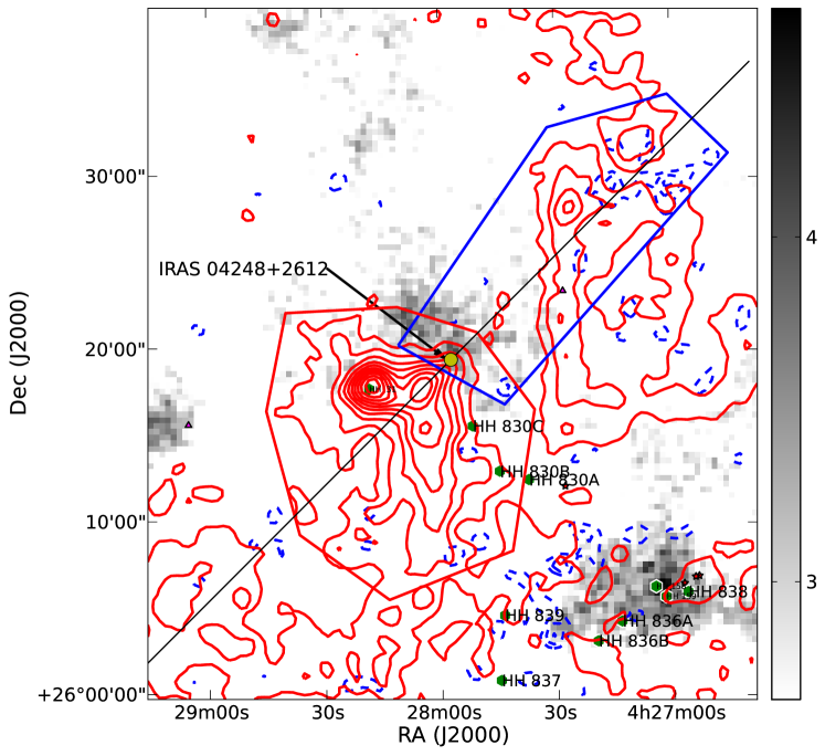
Figure 21: Contour map of blueshifted and redshifted gas about a $40^{\prime}\times 45^{\prime}$ region near IRAS04248+2612. See Figure 3 for details on symbols and markers. ¹²CO blueshifted and redshifted integrated intensity is for velocities of 0 to 3.6 km s^-1 and 8.1 to 13 km s^-1 respectively. Blueshifted contours range from 0.43 to 2.0 in steps of 0.075 K km s^-1, and redshifted contours range from 0.43 to 6.6 in steps of 0.075 K km s^-1.

Figure 22: Position velocity of ¹²CO emission towards the IRAS-4239+2612 region, through the slice at p.a. of $45^{\circ}$ shown in Figure 21. The contour range is 0.15 to 3.95 K in steps of 0.3 K. Shown in dashed line is the position of the yellow circle shown in Fig 21.

Figure 23: Average Spectra of ¹²CO emission (blue solid lines) and ¹³CO (green dashed lines) towards the blueshifted (left) and redshifted (right) lobes of the outflow in the IRAS04248+2612 region shown in Fig 21. The temperature scale is in T${}_{A}^{*}$.

3.1.8 Haro 6-10

The first evidence for high velocity gas in this region was provided by a snap-shot interferometer survey by Terebey et al. (1989). A small map of this region in the J=3-2 line of CO was made by Hogerheijde et al. (1998) and revealed a bipolar outflow. This region was subsequently mapped more extensively by Stojimirović et al. (2007) in the CO J=1-0 line and a large bipolar outflow was detected. This outflow is associated with a giant Herbig-Haro flow centred on Haro 6-10 (Devine et al., 1999). Haro 6-10 is also called GV Tau.

Figure 24 shows the redshifted and blueshifted emission in this region from our data. The distribution of high velocity emission is very similar to what was found by Stojimirović et al. (2007). The position-velocity map along the cut marked in Figure 24 is presented in Figure 25 and shows weak redshifted and blue shifted outflow emission. The polygon averaged spectra, shown in Figure 26, also show evidence for weak high velocity redshifted and blueshifted emission.

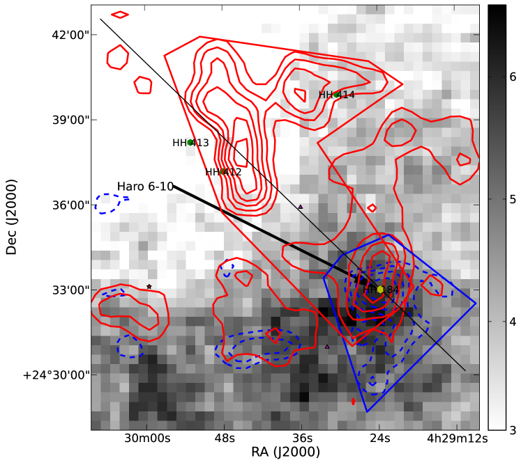
Figure 24: Contour map of blueshifted and redshifted gas about a $15^{\prime}\times 15^{\prime}$ region near Haro 6-10. See Figure 3 for details on symbols and markers. ¹²CO blueshifted and integrated intensity are for velocities of 0 to 3.5 km s^-1 and 8.5 to 12 km s^-1 respectively. Blueshifted contours range from 0.39 to 1.7 in steps of 0.075 K km s^-1, and redshifted contours range from 0.39 to 2.3 in steps of 0.075 K km s^-1.

Figure 25: Position velocity of ¹²CO emission towards the Haro 6-10 region, through the slice at p.a. of $136^{\circ}$ shown in Figure 24. The contour range is 0.1 to 4.3 K in steps of 0.3 K. Shown in dashed line is the position of the yellow circle shown in Fig 24.

Figure 26: Average Spectra of ¹²CO emission (blue solid lines) and ¹³CO (green dashed lines) towards the blueshifted (left) and redshifted (right) lobes of the outflow towards the Haro 6-10 region shown in Fig 24. The temperature scale is in T${}_{A}^{*}$.

3.1.9 IRAS 04278+2435 (ZZ Tau IRS)

Extended high velocity redshifted emission was found in the region around IRAS 04278+2435 by Heyer et al. (1987) and they associated this monopolar outflow with the pre-main sequence star ZZ Tau. The catalogue of YSOs of Kenyon et al. (2008) lists both ZZ Tau AB and ZZ Tau IRS (IRAS 04278+2435) that are separated by less than 1 arcminute, and either, based on the morphology of the outflow, may be the origin of this flow. This outflow has a distinct redshifted velocity feature similar to that seen in the L1551 IRS 5 outflow (Snell et al., 1980), and as in L1551 IRS 5 may be evidence for a swept-up shell. Their map revealed little evidence for any significant blueshifted emission. Gomez et al. (1997) detected a [SII] emission knot (HH 393) in this region and argue that ZZ Tau IRS is the most likely driving source for this outflow.

Our map of the high velocity emission is shown in Figure 27. We detect only redshifted emission and the morphology of this emission is similar to that found by Heyer et al. (1987). A position-velocity map along the line marked in Figure 27 is shown in Figure 28 where the distinct velocity feature at about 11 km s^-1 can be readily seen. Averaged spectra are shown in Figure 29 which shows clear high velocity redshifted emission. A polygon was selected where we might expect blueshifted emission to be present and the averaged spectra shows some evidence for high velocity blueshifted emission that may indicate that this is a asymmetrical bipolar outflow.

Figure 27: Contour map of blueshifted and redshifted gas about a $15^{\prime}\times 15^{\prime}$ region near ZZ Tau. See Figure 3 for details on symbols and markers. ¹²CO blueshifted and redshifted integrated intensity is for velocities of 0 to 3.5 km s^-1 and 8.5 to 12 km s^-1 respectively. Blueshifted contours range from 0.42 to 1.7 in steps of 0.075 K km s^-1, and redshifted contours range from 0.42 to 2.8 in steps of 0.075 K km s^-1.

Figure 28: Position velocity of ¹²CO emission towards the ZZ Tau region, through the slice at p.a. of $40^{\circ}$ shown in Figure 27. The contour range is 0.13 to 3.93 K in steps of 0.3 K. Shown in dashed line is the position of the yellow circle shown in Fig 27.

Figure 29: Average Spectra of ¹²CO emission (blue solid lines) and ¹³CO (green dashed lines) towards the presumed blueshifted (left) and redshifted (right) lobes of the outflow towards the ZZ Tau region shown in Fig 27. The temperature scale is in T${}_{A}^{*}$.

3.1.10 Haro 6-13

TMC-2A is one of the Taurus cloud cores identified by Myers et al. (1983) and in the vicinity of this core are four IRAS sources, three known to be associated with pre-main sequence stars (Kenyon et al., 2008): 04288+2417 (HK Tau), 04292+2422 (Haro 6-13) and 04294+2413 (FY/FZ Tau). Both 04288+2417 and 04292+2422 were studied by Heyer et al. (1987), Myers et al. (1988) and Moriarty-Schieven et al. (1994) and all found little evidence for high velocity gas toward these sources. Recently, Jiang et al. (2002) mapped the CO J=3-2 emission in this region and found extended high velocity emission. The most prominent high velocity emission forms a bipolar outflow roughly centred on IRAS 04292+2422 (Haro 6-13). This outflow was labeled TMC2A in the catalogue of Wu et al. (2004). The outflow emission is complicated and Jiang et al. (2002) suggest that there may be multiple outflows in the region.

Our map of the high velocity red and blue emission is shown in Figure 30 and the distribution of high velocity emission is similar to that presented in Jiang et al. (2002). A large bipolar outflow is clearly present and Haro 6-13, although slightly offset to the south-east of the centroid of the outflow, is most likely the driving source for this outflow. The redshifted gas is much more prominent than the blueshifted gas and that can be better seen in the p-v diagram shown in Figure 31. Averaged spectra are shown in Figure 32 which reveal relatively low velocity outflow emission.

The redshifted and blueshifted features near the Class 0 object HK Tau are suggestive of an outflow (see Figure 30), but do not meet our criteria for being an outflow.

Figure 30: Contour map of blueshifted and redshifted gas about a $25^{\prime}\times 25^{\prime}$ region near HK Tau. See Figure 3 for details on symbols and markers. ¹²CO blueshifted and redshifted integrated intensity is for velocities of 0 to 4.0 km s^-1 and 8.5 to 12 km s^-1 respectively. Blueshifted contours range from 0.39 to 1.83 in steps of 0.075 K km s^-1, and redshifted contours range from 0.4 to 4.0 in steps of 0.075 K km s^-1.

Figure 31: Position velocity of ¹²CO emission towards the HK Tau region, through the slice at p.a. of $60^{\circ}$ shown in Figure 30. The contour range is 0.13 to 3.93 K in steps of 0.3 K. Shown in dashed line is the position of the yellow circle shown in Fig 30.

Figure 32: Average Spectra of ¹²CO emission (blue solid lines) and ¹³CO (green dashed lines) towards the blueshifted (left) and redshifted (right) lobes of the outflow towards the HK Tau region shown in Fig 30. The temperature scale is in T${}_{A}^{*}$.

3.1.11 IRAS 04325+2402

This outflow is located in the L1535 cloud and was first detected and mapped in the CO J=1-0 line by Heyer et al. (1987). Only redshifted high velocity emission was detected in this outflow, however the outflow is quite large with an angular size of about 15 arcminutes. IRAS 04325+2402 is at the apex of this one-sided outflow. This source was in the survey of Moriarty-Schieven et al. (1992), who found a total line width of 13.9 km s^-1.

Our map of the high velocity emission is shown in Figure 33. We detect only redshifted emission and the morphology of the outflow is very similar to that found by Heyer et al. (1987). The protostellar source IRAS 04325+2402 is assumed to be the origin of this outflow. This protostellar source is complex with at least two components and a complex bipolar scattered light nebula (Hartmann et al., 1999). Sources A/B are located at the apex of the bipolar nebula, however its orientation is not consistent with the molecular outflow. Hartmann et al. (1999) suggest that the expected outflow from a fainter component C may be better aligned with the monopolar molecular outflow.

In Figure 34 a position-velocity map along the line marked in Figure 33 shows the prominent redshifted outflow emission. The redshifted outflow has a distinct secondary velocity feature at 8 km s^-1 located approximately 13 arcminutes north-west of IRAS 04325+2402. This feature may be part of shell-like structure, similar to the ZZ Tau outflow. Averaged spectra, shown in Figure 35, show clearly the high velocity redshifted outflow and only very weak evidence for any blueshifted emission.

Figure 33: Contour map of blueshifted and redshifted gas about a $25^{\prime}\times 25^{\prime}$ region near IRAS04325+2402. See Figure 3 for details on symbols and markers. ¹²CO blueshifted and redshifted integrated intensity is for velocities of -1 to 3.8 km s^-1 and 8.5 to 12 km s^-1 respectively. Blueshifted contours range from 0.43 to 2.1 in steps of 0.075 K km s^-1, and redshifted contours range from 0.43 to 2.5 in steps of 0.075 K km s^-1.

Figure 34: Position velocity of ¹²CO emission towards the IRAS04325+2402 region, through the slice at p.a. of $40^{\circ}$ shown in Figure 33. The contour range is 0.11 to 5.1 K in steps of 0.3 K. Shown in dashed line is the position of the yellow circle shown in Fig 33.

Figure 35: Average Spectra of ¹²CO emission (blue solid lines) and ¹³CO (green dashed lines) towards the blueshifted (left) and redshifted (right) lobes of the outflow seen towards IRAS04325+2402 region shown in Fig 33. The temperature scale is in T${}_{A}^{*}$.

3.1.12 HH 706 Outflow

A newly discovered bipolar outflow is found associated with the Herbig-Haro object HH 706 (Sun et al., 2003). We have labeled this molecular outflow HH 706 Outflow, as we were unable to identify in the Spitzer catalogue any source that might drive this outflow. See the overview figure of the Heiles Cloud 2 region in Figure 2 for the location of the HH 706 flow in this region. The distribution of redshifted and blueshifted gas toward HH 706 is shown in Figure 36. The blueshifted emission is much more extended than the redshifted emission and HH 706 is located at the centre of the region of strong redshifted high velocity emission. A p-v plot along the axis shown in Figure 36 is presented in Figure 37. The p-v plot shows prominent redshifted emission, while the blueshifted outflow has lower velocity and is less well delineated. The averaged spectra shown in Figure 38 show weak high velocity redshifted and blueshifted emission.

Figure 36: Contour map of blueshifted and redshifted gas about a $35^{\prime}\times 45^{\prime}$ region centred at RA of 04:39:35 and Dec of 25:25:16. See Figure 3 for details on symbols and markers. ¹²CO blueshifted and redshifted integrated intensity are for velocities of -1 to 4.0 km s^-1 and 8 to 13 km s^-1 respectively. Blueshifted contours range from 0.59 to 2.7 in steps of 0.075 K km s^-1, and redshifted contours range from 0.59 to 9.4 in steps of 0.075 K km s^-1.

Figure 37: Position velocity of ¹²CO emission towards the HH706 region, through the slice at p.a. of $0^{\circ}$ shown in Figure 36. The contour range is 0.1 to 5.3 K in steps of 0.2 K. Shown in dashed line is the position of the yellow circle shown in Fig 36.

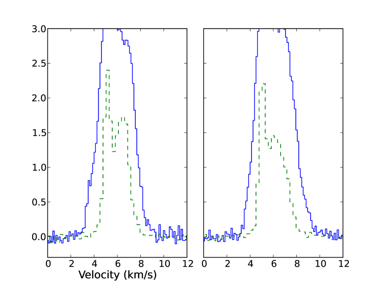
Figure 38: Average Spectra of ¹²CO emission (blue solid lines) and ¹³CO (green dashed lines) towards the blueshifted (left) and redshifted (right) lobes of the outflow seen towards HH706 region shown in Fig 36. The temperature scale is in T${}_{A}^{*}$.

3.1.13 HH 705 Outflow

The bipolar molecular outflow associated with HH 705 (Sun et al., 2003) is newly discovered. The distribution of redshifted and blueshifted emission is shown in Figure 39. The Herbig-Haro object HH 705 is located at the centroid of this bipolar outflow. McGroarty & Ray (2004) suggested that HH 705 could be associated with HV Tau C, however more recent proper motion measurements (McGroarty et al., 2007) seem to rule out this possibility. The proper motion measurements show that the four knots that compose HH 705 are moving to the south and southwest with velocities varying from 100 to 300 km s^-1. There is also [SII] and H$\alpha$ emission that extends nearly 2 arcminutes south of HH 705 McGroarty & Ray (2004). Further south along the bipolar outflow axis lies HH 831 and HH 832 (McGroarty & Ray, 2004), however the proper motion vectors for HH 831A are directly westward, while those for HH 831B are directed southeast (McGroarty et al., 2007). It is unclear whether these Herbig-Haro objects are related to this large bipolar outflow. The driving source for the large molecular outflow and HH 705 is unknown. We have labeled this molecular outflow HH 705 Outflow.

The p-v plot along the axis defined in Figure 39 is shown in Figure 40. The bipolar nature of this outflow can be clearly seen as well as its large extend of nearly 20 arcminutes. The averaged spectra in the two polygons are shown in Figure 41 and also show clearly the high velocity blueshifted and redshifted gas associated with this outflow.

Figure 39: Contour map of blueshifted and redshifted gas about a $35^{\prime}\times 45^{\prime}$ region centred at RA of 04:39:07 and Dec of 26:17:20. See Figure 3 for details on symbols and markers. ¹²CO blueshifted and redshifted integrated intensity are for velocities of -1 to 3.9 km s^-1 and 8.3 to 13 km s^-1 respectively. Blueshifted contours range from 0.57 to 2.3 in steps of 0.075 K km s^-1, and redshifted contours range from 0.57 to 3.5 in steps of 0.075 K km s^-1.

Figure 40: Position velocity of ¹²CO emission towards the HH705 region, through the slice at p.a. of $85^{\circ}$ shown in Figure 39. The contour range is 0.1 to 5.3 K in steps of 0.2 K. Shown in dashed line is the position of the yellow circle shown in Fig 39.

Figure 41: Average Spectra of ¹²CO emission (blue solid lines) and ¹³CO (green dashed lines) towards the blueshifted (left) and redshifted (right) lobes of the outflow seen towards HH705 region shown in Fig 39. The temperature scale is in T${}_{A}^{*}$.

3.1.14 TMR-1 (IRAS 04361+2547)

Based on their small interferometer map of the CO J=1-0 emission, Terebey et al. (1990) were first to detect an outflow associated IRAS 04361+2547, which they labeled TMR-1. In the J=3-2 CO line toward this source, Moriarty-Schieven et al. (1992) measured a total line-width of 14.7 km s^-1. A region larger than that observed by Terebey et al. (1990) was mapped by Bontemps et al. (1996) in the CO J=2-1 line and Hogerheijde et al. (1998) in the CO J=3-2 line, and these studies revealed that this outflow was extended on angular scales of at least 2 arcminutes, however no clear bipolar morphology was seen. Terebey et al. (1998) resolved TMR-1 into a binary (TMR-1AB) that is surrounded by extended nebulosity. Near infrared images of this region (Petr-Gotzens et al., 2010) reveal nebulosity extended south-east and north-west of IMR-1. Near infrared spectra of the emission to the south-east shows emission lines of molecular hydrogen which Petr-Gotzens et al. (2010) interpret as shocked excited. Thus there is strong evidence for a extended shocked gas emission directed to the southeast of TMR-1AB.

Our map of the high velocity redshifted and blueshifted emission is shown in Figure 42. We detect primarily blueshifted emission associated with this outflow, similar to the maps of Bontemps et al. (1996) and Hogerheijde et al. (1998), although the outflow emission is somewhat more extended. We also see weak blueshifted emission extending to the east of TMR-1, however it is unclear whether this is related to the TMR-1 outflow. The p-v plot along the direction marked in Figure 42 is shown in Figure 43. Prominent blueshifted emission is seen, but no evidence is seen for redshifted emission. Likewise the averaged spectra show blueshifted emission, but no sign of redshifted emission. The redshifted emission shown in the plots of Bontemps et al. (1996) is for a velocity range of 6 to 8.6 km s^-1 that may be strongly contaminated by the ambient cloud emission.

Figure 42: Contour map of blueshifted and redshifted gas about a $20^{\prime}\times 20^{\prime}$ region centred at RA of 04:39:44 and Dec of 25:56:00. See Figure 3 for details on symbols and markers. ¹²CO blueshifted and redshifted integrated intensity are for velocities of -1 to 4.1 km s^-1 and 8.1 to 13 km s^-1 respectively. Blueshifted contours range from 0.63 to 3.0 in steps of 0.075 K km s^-1, and redshifted contours range from 0.63 to 5.6 in steps of 0.075 K km s^-1. Three outflows are seen in the figure, those due to TMR1, L1527 and IC2087 (the latter being the central big redshifted lobe).

Figure 43: Position velocity of ¹²CO emission towards the TMR1 region, through the slice at p.a. of $85^{\circ}$ shown in Figure 42. The contour range is 0.12 to 5.32 K in steps of 0.2 K. Shown in dashed line is the position of the yellow circle shown in Fig 42.

Figure 44: Average Spectra of ¹²CO emission (blue solid lines) and ¹³CO (green dashed lines) towards the blueshifted (left) and redshifted (right) lobes of the outflow seen towards the TMR1 region shown in Fig 42. The temperature scale is in T${}_{A}^{*}$.

3.1.15 L1527 (IRAS 04368+2557)

IRAS 04368+2557 is also called L1527 IRS (Kenyon et al., 2008). As in many of these outflows, the first evidence for high velocity gas came from the CO J=3-2 survey of Moriarty-Schieven et al. (1992) who found a total line width of 19.4 km s^-1 towards this source. Subsequent maps by Bontemps et al. (1996), Tamura et al. (1996) and Zhou et al. (1996) revealed a small bipolar outflow oriented east-west. More extensive mapping by Hogerheijde et al. (1998) showed that the bipolar outflow had an angular extent of approximately 4 arcminutes, much larger than was suspected from the earlier observations. Their outflow map showed significant overlap between the redshifted and blueshifted high velocity emission implying a large inclination angle as was first suggested by Tamura et al. (1996).

There is also evidence for an optical jet from this source based on the emission line nebulosity located east of L1527 IRS Eiroa et al. (1994). A series of Herbig-Haro objects (HH 192 A,B,C) are located on either side of L1527 IRS oriented east-west along the molecular outflow axis (Gomez et al., 1997). L1527 IRS is also known to have a flattened, nearly edge on disk seen in molecular emission (Ohashi et al., 1997) and in scattered light imaging (Tobin et al., 2010).

Our map of the high velocity emission is shown in the top part of Figure 42. We see a bipolar outflow oriented east-west with a morphology and angular size similar to that seen in Hogerheijde et al. (1998). An east-west p-v plot is presented in Figure 45 showing a clear bipolar signature. Averaged spectra are shown in Figure 46 and along with the p-v plot reveal weak and relatively low velocity outflow emission.

Figure 45: Position velocity of ¹²CO emission towards the L1527 region, through the slice at p.a. of $0^{\circ}$ through L1527 shown in Figure 42. The contour range is 0.1 to 5.3 K in steps of 0.2 K. Shown in dashed line is the position of the yellow circle shown in Fig 42.

Figure 46: Average Spectra of ¹²CO emission (blue solid lines) and ¹³CO (green dashed lines) towards the blueshifted (left) and redshifted (right) lobes of the outflow seen towards the L1527 region shown in Fig 42. The temperature scale is in T${}_{A}^{*}$.

3.1.16 IRAS 04369+2539 (IC 2087 IR)

Heyer et al. (1987) first detected high velocity redshifted emission associated with IRAS 04369+2539. Their maps revealed a one-sided, redshifted only outflow with an angular extent of 14 arcminutes. An extended reflection nebula, IC 2087, is associated with this source and the YSO is often refered to as IC 2087 IR. Also associated with this outflow are the two Herbig-Haro objects HH 395A and HH 395B (Gomez et al., 1997) located approximately 2 arcmin north-east of IC 2087 IR. The relationship of these Herbig-Haro objects to the outflow is unclear.

Our map of the high velocity redshifted and blueshifted emission is shown in Figure 47. The distribution of redshifted outflow emission is very similar to that shown in Heyer et al. (1987). A p-v plot along the axis through IC 2087 IR, marked in Figure 47 is shown in Figure 48 and shows prominent redshifted emission. Spectra averaged within the polygons shown in Figure 47 are shown in Figure 49, and like the p-v plot, show prominent redshifted emission and little evidence for blueshifted high velocity emission.

Figure 47: Contour map of blueshifted and redshifted gas about a $25^{\prime}\times 25^{\prime}$ region centred at RA of 04:39:45 and Dec of 25:49:00. Two outflows, IC 2087 and TMC1A can be seen in the figure. See Figure 3 for details on symbols and markers. ¹²CO blueshifted and redshifted integrated intensity are for velocities of -1 to 3.9 km s^-1 and 8.2 to 13 km s^-1 respectively. Blueshifted contours range from 0.66 to 2.7 in steps of 0.075 K km s^-1, and redshifted contours range from 0.66 to 5.4 in steps of 0.075 K km s^-1.

Figure 48: Position velocity of ¹²CO emission towards the IC2087 region, through the slice at p.a. of $65^{\circ}$ through IRAS 04369+2539 shown in Figure 42. The contour range is 0.12 to 5.32 K in steps of 0.2 K. Shown in dashed line is the position of the yellow circle shown in Fig 47.

Figure 49: Average Spectra of ¹²CO emission (blue solid lines) and ¹³CO (green dashed lines) towards the blueshifted (left) and redshifted (right) lobes of the outflow seen towards the IC2087 region shown in Fig 47. The temperature scale is in T${}_{A}^{*}$.

3.1.17 IRAS 04365+2535 (TMC-1A)

This outflow is located in the TMC 1A core, hence its name. The first evidence for high velocity gas was provided in the snap-shot interferometer survey by Terebey et al. (1989). This sources was observed by Moriarty-Schieven et al. (1992), who found a total line width of 29.8 km s^-1 in the CO J=3-2 line, however the line was asymmetrical with much higher blueshifted velocities than redshifted. Tamura et al. (1996), Chandler et al. (1996), Bontemps et al. (1996) and Hogerheijde et al. (1998) all mapped this region revealing an outflow centred on the IRAS source and extended on angular scales of at least 2 arcminutes. The outflow is bipolar, however the redshifted emission is very weak.

Our map of the high velocity emission is shown in the same figure as the IC 2087 outflow (see Figure 47, and is the small outflow to the bottom right). We detect only blueshifted emission. This outflow is very small with weak emission and is near our threshold for outflow detection. A p-v plot is shown in Figure 50 and averaged spectra in Figure 51, and in both figures only weak blueshifted emission is detected.

Figure 50: Position velocity of ¹²CO emission towards the TMC1A region, through the slice at p.a. of $75^{\circ}$ through IRAS 04365+2535 shown in Figure 47. The contour range is 0.12 to 4 K in steps of 0.15 K. Shown in dashed line is the position of the yellow circle shown in Fig 47.

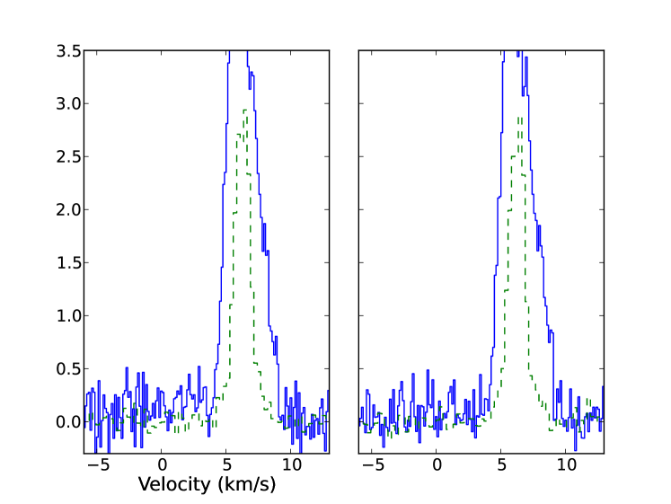
Figure 51: Average Spectra of ¹²CO emission (blue solid lines) and ¹³CO (green dashed lines) towards the blueshifted (left) and redshifted (right) lobes of the outflow seen towards the TMC1A region shown in Fig 47. The temperature scale is in T${}_{A}^{*}$.

3.1.18 TMC-1 North Outflow

We have detected a new outflow with a striking blueshifted emission north of the core TMC-1. The outflow is located approximately 12 arcminutes east of HH 705 Outflow and 20 arcminutes north of IC 2087 IRS (see Figure 2). We label this outflow TMC-1 North Outflow. A map of the high velocity emission is shown in Figure 52. This blueshifted only outflow is highly collimated and has an angular extent of nearly 20 arcminutes. There is no known YSO in the vicinity, thus the source of this outflow is unknown. We have chosen a position at the south end of the outflow as the outflow centroid, and this position is given in Table 2. This position is close to one of the high extinction regions from the data of Padoan et al. (2002) and shown in Tóth et al. (2004). We show a p-v plot along the path marked in Figure 52 in Figure 53 and this plot shows clear evidence for high velocity blueshifted emission. The averaged spectra are shown in Figure 54, again clear evidence is seen for high velocity blueshifted gas, however in the polygon south of the chosen outflow centroid, no redshifted emission is detected.

Figure 52: Contour map of blueshifted and redshifted gas about a $35^{\prime}\times 35^{\prime}$ region in the region around TMC-1 North. See Figure 3 for details on symbols and markers. ¹²CO blueshifted and integrated intensity are for velocities of -1 to 4.1 km s^-1 and 8.1 to 13 km s^-1 respectively. Blueshifted contours range from 0.6 to 2.5 in steps of 0.075 K km s^-1, and redshifted contours range from 0.6 to 3.6 in steps of 0.075 K km s^-1.

Figure 53: Position velocity of ¹²CO emission towards the TMC-1 North region, through the slice at p.a. of $80^{\circ}$ shown in Figure 42. The contour range is 0.12 to 5.32 K in steps of 0.2 K. Shown in dashed line is the position of the yellow circle shown in Fig 52.

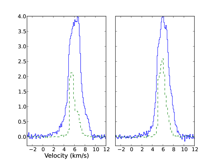
Figure 54: Average Spectra of ¹²CO emission (blue solid lines) and ¹³CO (green dashed lines) towards the blueshifted (left) and redshifted (right) lobes of the outflow seen towards the TMC-1 North region shown in Fig 52. The temperature scale is in T${}_{A}^{*}$.

3.1.19 IRAS 04381+2540 (TMC 1)

IRAS 04381+2540 is located in the TMC 1 core. Evidence for high velocity gas was first found by Moriarty-Schieven et al. (1992) who measured a total line width of 36.6 km s^-1 in the CO J=3-2 line toward this source. This region was subsequently mapped by Bontemps et al. (1996). Chandler et al. (1996) and Hogerheijde et al. (1998) who all found a small bipolar outflow centred on this IRAS source with an angular extent of about 1.5 arcminutes. Infrared imaging (Apai et al., 2005; Terebey et al., 2006) reveal a narrow jet and a wide-angle conical outflow cavity. The jet, first seen by Gomez et al. (1997), is directed nearly due north of the YSO.

Our maps of the high velocity emission are shown in Figure 55 and reveal an outflow much more spatially extended than previous maps. The outflow near the central source is nearly north-south, but the redshifted emission is extended nearly 20 arcminutes from the central source and curves to the south-east. The blueshifted emission is much weaker and the morphology of this part of the outflow poorly determined. The p-v plot along the line marked in Figure 55 is shown in Figure 56. The p-v plot shows the extended nature of the redshifted lobe of the outflow, however it misses some of the more intense regions of redshifted and blueshifted emission. The averaged spectra shown in Figure 57 shows clearly the redshifted outflow emission, but the blueshifted emission is much weaker.

Figure 55: Contour map of blueshifted and redshifted gas about a $45^{\prime}\times 45^{\prime}$ region centred on TMC1. See Figure 3 for details on symbols and markers. ¹²CO blueshifted and redshifted integrated intensity are for velocities of -1 to 4.1 km s^-1 and 8. to 13 km s^-1 respectively. Blueshifted contours range from 0.61 to 2.8 in steps of 0.075 K km s^-1, and redshifted contours range from 0.61 to 4.4 in steps of 0.075 K km s^-1.

Figure 56: Position velocity of ¹²CO emission towards the TMC1 region, through the slice at p.a. of $65^{\circ}$ shown in Figure 42. The contour range is 0.12 to 5.32 K in steps of 0.2 K. Shown in dashed line is the position of the yellow circle shown in Fig 55.

Figure 57: Average Spectra of ¹²CO emission (blue solid lines) and ¹³CO (green dashed lines) towards the blueshifted (left) and redshifted (right) lobes of the outflow seen towards the TMC1 region shown in Fig 55. The temperature scale is in T${}_{A}^{*}$.

3.1.20 Source 045312+265655

Our outflow search process yielded a surprising detection of a possible outflow at RA of 04:43:12 and Dec of 26:56:55 (J2000). We call this outflow Source 045312+265655. Figure 58 shows a map of the high velocity emission towards this region. There are no known YSOs in this area, although it is very likely that the Spitzer survey did not cover this particular region. This outflow is curious in a variety of ways. There is little ambient gas around to sweep up as there is almost no detectable ¹³CO emission. The position velocity diagram shown in Figure 59 reveals a canonical outflow signature. The averaged spectra in the blue and redshifted polygonal regions (Figure 60) show high velocity wings in blue and redshifted gas. So it is no wonder that our outflow detection algorithm picked up this source. But it is very atypical in that we cannot attribute any known driving source for this outflow. Moreover, it is hard to conceive how a YSO could even form in such low column density regions.

This region in the north-east section of the Taurus Molecular Cloud is the same region studied by Heyer et al. (2008), where they found the low column density substrate of gas with striations of elevated ¹²CO gas that is well aligned with local magnetic field direction.

Figure 58: Contour map of blueshifted and redshifted gas about a $20^{\prime}\times 20^{\prime}$ region centred on RA 04:53:12 and Dec 26:56:55. No detectable ¹³CO emission greater than 10 sigma is detected in this region. See Figure 3 for details on symbols and markers. ¹²CO blueshifted and redshifted integrated intensity are for velocities of -1 to 4.3 km s^-1 and 7.8 to 13 km s^-1 respectively. Blueshifted contours range from 0.6 to 2. in steps of 0.075 K km s^-1, and redshifted contours range from 0.6 to 2.4 in steps of 0.075 K km s^-1.

Figure 59: Position velocity of ¹²CO emission towards the region shown in Figure 58, through the slice at p.a. of $155^{\circ}$ shown in that figure. The contour range is 0.12 to 5.32 K in steps of 0.2 K. Shown in dashed line is the position of the yellow circle shown in Fig 58.

Figure 60: Average Spectra of ¹²CO emission (blue solid lines) and ¹³CO (green dashed lines) towards the blueshifted (left) and redshifted (right) lobes of the outflow seen towards the region shown in Fig 58. The temperature scale is in T${}_{A}^{*}$.

3.2 Outflows Not Detected

There are a number of previously identified outflows that were not detected in our survey. From the outflows in Table 1, we were unable to detect four of these even though they were within the region surveyed (IRAS 04181+2655, IRAS 04240+2559, L1529 and IRAS 04302+2247).

The outflow, IRAS 04181+2655 (CFHT-19), is a bipolar outflow first detected by Bontemps et al. (1996). The recent observations by Davis et al. (2010a) confirm the presence of a bipolar outflow in this region, which in Table 2 of their paper is labeled J04210795+2702204. This outflow is small and has relatively weak emission. The detections by Bontemps et al. (1996) and Davis et al. (2010a) were made in the CO J=2-1 and CO J=3-2 lines respectively. For warm, optically thin emission, as may be expected for outflows, the emission in these higher rotational transitions of CO should be stronger than in the CO J=1-0 line used in our survey. It is likely that this outflow is below our detection threshold.

Similarly, the redshifted only molecular outflow IRAS 04240+2559, detected by Mitchell et al. (1994), and associated with DG Tau, has very weak emission even in the CO J=3-2 line used in their study. We note that the CO J=3-2 spectrum obtained toward this source by Moriarty-Schieven et al. (1992) had very broad wings and had a total velocity extent of 29.9 km s^-1, so there is little doubt that an outflow is present. As in IRAS 04181+2655, this outflow must be below our detection threshold.

The L1529 outflow was detected by Lichten (1982) in the CO J=1-0 emission. He found high velocity emission toward two positions with full velocity extents as large as 30 km s^-1. The highest velocity emission was found in a region about 8 arcminutes south-east of Haro 6-13. This region was subsequently studied by Goldsmith et al. (1984) and their observations of the CO J=1-0 line did not confirm the presence of high velocity emission, although their sensitivity was sufficient to readily detect the high velocity emission reported by Lichten (1982). We also found no evidence for an outflow in our survey, so this outflow has never been confirmed and it’s existence is doubtful.

Finally, IRAS 04302+2247, which was mapped by Bontemps et al. (1996) in the CO J=2-1 line, was not detected in our survey. Their small map revealed a bipolar outflow with an irregular geometry. As in previous outflows, the emission is very weak and likely below our detection limit.

In addition to the outflows in Table 1, a number of additional outflow candidates were found by Davis et al. (2010a) in their CO J=3-2 map of the L1495 region. The outflows E-CO-R1, E-CO-R2, SE-CO-R1, SE-CO-R2, SE-CO-flow1, CFHT-21 and SE-CO-B1 were not identified as outflows in our survey.

3.3 Summary of Masses, Energy, etc.

To understand the effects of a molecular outflow in its immediate environment, it is important to calculate the mass, momentum, and mechanical energy output of the outflows as accurately as possible. The availability of both ¹²CO and ¹³CO data allow us to mitigate some issues that typically can cause rather large uncertainties in the estimation of the physical properties of outflows. One major issue is the confusion of the slow-moving parts of the outflow with the “ambient” gas at low velocities that are not part of the outflow. By judging the velocity extent of ¹³CO emission (which because of its lower abundance is predominantly seen only in the higher column density ambient gas), we try to avoid the ambient gas contamination by simply eliminating any emission at “low velocities”. That means that our mass and energetics are only lower limits, since we are probably missing outflowing gas projected to lower velocities with respect to the cloud’s LSR. Another major source of uncertainty in determining physical properties is the unknown inclination of the outflow axis to the plane of the sky. This problem is much harder to deal with. There are many methods of inclination correction in the outflow literature. The most robust method is to use proper motion studies of HH objects in the flow. Since most of our flows do not have corresponding HH objects, and proper motion studies do not exist for many of these flows, we chose to present the physical data of outflows uncorrected for inclination effects.

Table 3 lists the mass, momentum, energy, length and dynamical timescale of blue and redshifted lobes of the detected outflows. Our algorithm for the calculation of column densities is the same as that presented in Goldsmith et al. (2008). In the polygonal regions of the outflow contour figures presented above, we derive column density using both ¹²CO and ¹³CO for each pixel, and derive total blue-shifted and red-shifted column densities (after correcting for the relative antenna main beam efficiencies at each frequency, 0.5 and 0.45 respectively for ¹³CO and ¹²CO). We use an excitation temperature of 25 K. Our assumption of excitation temperature (25 K) could be lower or higher than the real value. For example, in Stojimirović et al. (2006), using the ratio of J=3-2 to J=1-0 of ¹²CO, they estimate an excitation temperature of 16.5 K for outflowing gas. Using this lower temperature will decrease the estimates of mass, momentum and energy by a factor of 1.3. However, Hirano & Taniguchi (2001) show that it is not uncommon for outflowing molecular gas to have excitation temperatures in the 50–100 K range. Using these higher values would increase our estimate of the outflow mass, momentum and energy by a factor of 1.7 to 3.1 for excitation temperature of 50 and 100 K respectively.

We also assume a ¹²CO to ¹³CO abundance ratio of 65, and an abundance of H₂ to ¹²CO of $1.1\times 10^{4}$. Column densities are then converted to mass using the distance to Taurus of 140 pc (Elias, 1978). Momentum and kinetic energy are estimated from average velocities in each lobe. The length of the outflow lobe is derived from the presumed driving source and the furthest extent of the contours shown in the figures. The dynamical timescale in Table 3 is derived simply from the length and the average velocity of the gas in each lobe.

It should be noted that the mass, momentum and energy listed in Table 3 are strictly lower limits, as there are several effects that have not been taken into account, which if properly estimated, would increase these quantities. The main effects that make our estimates lower limits can be listed as follows, and is similar to the arguments presented in Arce et al. (2010). We probably are missing a rather large fraction of low-velocity outflowing gas in our effort to avoid contamination with ambient cloud emission. We assign a factor of 2 for this unaccounted outflow emission. We are not correcting for angle of inclination effects. But if we assume that the average outflow is tilted by 45^∘ to the plane of the sky, then the momentum and energy are to be scaled up by factors of 1.4 and 2 respectively. Combining the factor of 2 due to missing outflowing gas at lower velocities and the factor of 2 due to inclination, the total scaling factor for outflow lobe momentum and energy will be as large as a factor of 2.8 and 4 respectively. So it may be fair to multiply the momentum and energy values listed in Table 3 by a factor of 2.8 and 4 respectively (however, the uncorrected numbers are listed in the Table). Assuming the average outflow is tilted by 45^∘, we can ignore any correction for the calculation of the dynamic age, t_dyn, since the correction for distance in the numerator and velocity in the denominator in estimating t_dyn cancel out.

Table 3: Outflow Mass, Velocity and Energy estimates

S.No	Name	Lobe	$v_{\rm avg}$	Mass	Momentum	Energy	Length	$t_{\rm dyn}$	Lflow
			km s-1	M⊙	M⊙km s-1	$\times 10^{43}$ (ergs)	pc	$10^{5}$ yrs	$\times 10^{30}$ (ergs/s)
1.	041149+294226	Blue	5.3	0.077	0.41	2.15	1.0	1.9	3.6
		Red	5.0	0.046	0.23	1.13	0.55	1.1	3.3
2.	IRAS 04113+2758	Blue	-	-	-	-	-	-	-
		Red	4.3	0.018	0.08	0.32	0.25	0.6	1.7
3.	IRAS 04166+2706	Blue	5.0	0.044	0.22	1.10	0.67	1.3	2.7
		Red	4.5	0.027	0.12	0.54	0.50	1.1	1.6
4.	IRAS 04169+2702	Blue	4.9	0.039	0.19	0.94	0.35	0.7	4.3
		Red	4.6	0.012	0.06	0.26	0.23	0.5	1.7
5.	FSTAU B	Blue	5.0	0.016	0.08	0.39	0.55	1.1	1.1
		Red	3.4	0.005	0.02	0.06	0.17	0.5	0.4
6.	IRAS 04239+2436	Blue	-	-	-	-	-	-	-
		Red	3.3	0.094	0.31	1.02	1.24	3.7	0.9
7.	IRAS 04248+2612	Blue	5.4	0.016	0.08	0.45	0.64	1.2	1.2
		Red	3.4	0.14	0.47	1.58	0.54	1.6	3.1
8.	Haro 6-10	Blue	4.4	0.005	0.02	0.10	0.17	0.4	0.8
		Red	4.2	0.02	0.09	0.35	0.44	1.0	1.1
9.	ZZ Tau IRS	Blue	-	-	-	-	-	-	-
		Red	4.4	0.023	0.10	0.44	0.30	0.7	2.0
10.	Haro 6-13	Blue	3.7	0.050	0.18	0.67	0.71	1.9	1.1
		Red	4.6	0.163	0.74	3.36	0.55	1.2	8.9
11.	IRAS04325+2402	Blue	-	-	-	-	-	-	-
		Red	4.5	0.077	0.35	1.56	0.83	1.8	2.8
12.	HH 706 flow	Blue	4.4	0.087	0.38	1.67	0.88	2.0	2.7
		Red	4.6	0.112	0.52	2.36	0.48	1.0	7.5
13.	HH 705 flow	Blue	4.5	0.014	0.06	0.27	0.46	1.0	0.9
		Red	4.8	0.062	0.29	1.39	0.43	0.9	4.9
14.	IRAS04361+2547	Blue	4.4	0.012	0.05	0.23	0.20	0.5	1.5
		Red	4.7	0.006	0.03	0.12	-	-	-
15.	TMC1A	Blue	4.5	0.002	0.01	0.04	0.07	0.2	0.6
		Red	4.7	0.004	0.02	0.09	0.07	0.1	2.9
16.	L1527	Blue	4.4	0.004	0.02	0.07	0.12	0.3	0.7
		Red	4.7	0.006	0.03	0.13	0.15	0.3	1.4
17.	IC2087 IR	Blue	4.5	0.001	0.01	0.02	-	-	-
		Red	4.7	0.135	0.63	2.94	0.65	1.4	6.7
18.	TMC-1 North	Blue	4.4	0.042	0.19	0.81	0.56	1.3	2.0
		Red	4.7	0.017	0.08	0.36	-	-	-
19.	TMC1	Blue	4.4	0.038	0.17	0.72	0.78	1.3	1.8
		Red	4.6	0.094	0.43	1.98	1.0	2.1	3.0
20.	045312+265655	Blue	4.3	0.003	0.01	0.05	0.14	0.3	0.5
		Red	4.5	0.007	0.03	0.13	0.21	0.5	0.8

4 Discussion

4.1 Parsec Scale Outflows in Taurus

A somewhat surprising result in the study of HH flows from young stars using larger format CCD cameras in the 1990s was that many of these flows could extend to many parsecs from the driving source (e.g. Bally & Devine, 1994; Reipurth et al., 1998). When large-scale millimetre wavelength molecular line mapping is performed, many molecular outflows were shown to extend to parsec scales, as well (e.g. Bence et al., 1996; Wolf-Chase et al., 2000; Arce et al., 2010). However, such millimetre wavelength mapping studies have been hampered by the large amounts of observational time required to adequately complete the projects. Hitherto, in most studies of molecular outflows from YSOs, even for the non parsec-scale ones, mapping of the flow has been done primarily in the main isotope of ¹²CO, with some opacity correction applied using pointed observations of ¹³CO.

With the advent of large-format heterodyne focal plane arrays like SEQUOIA (Erickson et al., 1999), it is now possible to make sensitive, large spatial extent, high spatial and velocity resolution maps at millimetre wavelengths that were hitherto not possible with finite amounts of observing time (Ridge et al., 2006; Narayanan et al., 2008). With the 100 square degree area covered by the Taurus Molecular Cloud Survey, it becomes possible to study the true extent of molecular outflows in this region. Knowledge of the true extent of outflows will in turn allow a more accurate assessment of the impact of outflows from YSOs on feedback mechanisms in molecular clouds, the role that outflows play in pumping and maintaining turbulence in these clouds.

Of the 20 outflows listed in Table 3, 8 outflows (40%) have a combined length of redshifted and blueshifted lobes that are greater than 1 pc in length. These 8 parsec-scale outflows have an average length of 1.37 pc. Four of these parsec-scale flows, 041159+294236, IRAS04248+2612, Haro 6-13, and HH 706 flow are new outflow detections. Even when the outflow is previously known and studied, our results indicate that they are considerably longer than previously suspected.

For example, in IRAS 04166+2706 (see Figure 10), the entire extent of the outflow previously studied in great detail by Santiago-García et al. (2009) is only a few arcminutes in length, and their maps are confined to regions close to the driving source. In this latter study, using high angular resolution data derived from interferometer and single-dish data, the authors are able to distinguish the detailed kinematic information for the oppositely directed winds and the swept-up shells. But what is being missed in the study by Santiago-García et al. (2009) is the mammoth scale of the 04166 outflow much beyond the region that they studied.

Our results suggest that a more careful census of outflowing gas using large-scale mapping studies such as done here will elucidate the true scales and reaches of molecular outflows and their impacts on GMCs.

4.2 Statistics of Outflows and Young Stars in Taurus

We have detected 20 outflow sources in the Taurus Molecular Cloud of which 8 are new identifications. Given that our sensitivity limits prevent the identification of at least 3 other sources (see §3.2), we can postulate that there are at least 23 outflow sources in Taurus. The Spitzer map of Taurus (Rebull et al., 2010), while not covering all of the mapped Taurus Molecular Cloud, has 215 YSOs in the previously known candidate list, and 148 new YSOs as newly identified candidates. In the Rebull et al. (2010) catalogue, YSOs are classified as Class I, Flat, Class II or Class III based on the slope of the spectral energy distribution (SED). Since Spitzer observations cannot distinguish Class 0 objects from Class I (and the most embedded Class 0 objects may not be detected by Spitzer), we can assume that the Class I and Flat spectrum sources represent the most embedded and youngest population of YSOs, with the Class I objects forming the younger subset. Of the Spitzer detected YSOs, there are 48 Class I objects and 33 Flat spectrum objects. There are thus 81 total embedded objects in a list of 363 YSOs ($\sim 22$%) in the Spitzer catalogue.

Of the 23 outflow sources in Taurus, 18 can be associated with known Spitzer identifications, and their spectral classification can be derived. Table 2 lists this SED class in the YSO class column. The remaining 5 outflow sources are all new detections from this study, and all but one (045312+265655), are in the regions covered by Spitzer, so the Spitzer non-detection of the driving sources might imply that these are Class 0 sources. The three non-detected outflows of this study (see §3.2) are all classified as Class I sources. Of the 18 outflows with identified driving sources, 14 are Class I objects, and 4 are Flat spectrum objects. We conclude from this that $\sim 30$% of Class I sources and $\sim 12$% of Flat spectrum sources in Taurus have outflows. Recently, a comprehensive list of known Class 0 protostars was compiled (Froebrich, 2005), and the list is being actively maintained as a Class 0 database online. This list contains five Class 0 protostars in the Taurus region surveyed: B213 (what they refer to as PS041943.00+271333.7, which is also IRAS04166+2706), L1521-F IRS, IRAS 04248+2417 (HK Tau), IRAS 04325+2402 (L1535) and IRAS 04368+2557 (L1527). Of these five sources, three of the objects, IRAS04166+2706, L1535 and L1527 are outflows detected in this study. In the Spitzer classification of Rebull et al. (2010), HK Tau (IRAS 04248+2417) is actually classified as a Class II object, which is also confirmed by recent Akari observations (Aikawa et al., 2012). Stapelfeldt et al. (1998) using Hubble Space Telescope observations found HK Tau to be an edge-on disk, which may explain its mis-classification as a Class 0 object in the online database. So we drop HK Tau from the list of Class 0 objects in Taurus. L1521-F IRS is known to be a very low-luminosity source which is probably a very young Class 0 object (Terebey et al., 2009). We detect no outflow towards L1521-F. We conclude that 75% of known Class 0 objects in Taurus have outflows.

But what could explain the non-detection of outflows towards 63 other Spitzer-detected embedded Class I and Flat spectrum sources in Taurus? It is possible that our sensitivity limits and our relatively coarse angular resolution prevents the identification of small-scale, low intensity flows. But it is more likely that these 63 embedded sources without outflows represent an older population, where the swept-up molecular outflows have slowed down to ambient cloud velocities, and are hence not detectable in high-velocity wings. The mean dynamic age of the outflows in our study is $1.1\times 10^{5}$ years, with the maximum being $3.7\times 10^{5}$ years. When compared against the average lifetime of about $5\times 10^{5}$ years for the Class I protostellar phase (Evans et al., 2009), the non-detection of outflows in a large number of Class I and Flat spectrum sources in Taurus could mean that molecular outflows are a short-lived phenomenon marking the youngest phase of protostellar life.

4.3 Turbulence in Molecular Cloud and Outflows as Injection Mechanism

The sources of turbulent motions in molecular clouds have been intensely debated over the past three decades (see for e.g. from Larson, 1981; Heyer & Brunt, 2004). At larger scales, kinetic energy injection from supernovae and galactic differential rotation can provide sources of turbulent energy. At smaller scales, stellar feedback in the form of HII regions, radiatively driven winds, and accretion-driven outflows are believed to be the sources of turbulent energy. The question of what powers the turbulence is important. However, questions on the so-called injection scale of turbulence, and whether there is in fact more than one injection scale where energy is deposited into the turbulent spectrum are equally important. Another unanswered question is what sustains the turbulence in the parsec and sub-parsec scale clumps. It is clear that the turbulence needs to be driven continually over timescales longer than the crossing time either internally using stellar feedback processes, or externally using some cascade down process from the ISM.

A very different question from the origin of turbulent motions in star-forming clouds is the role that turbulence provides during the star-formation process. In the absence of turbulent support, most of the mass within a given structure, be it a GMC, cloud or core, would collapse into stars within one free-fall time with an efficiency per free fall time, $\epsilon_{\rm ff}$ approaching 1 (see Krumholz & McKee, 2005; McKee & Ostriker, 2007, for definition of $\epsilon_{\rm ff}$). However, direct observations provide very low values of $\epsilon_{\rm ff}$ ranging from 0.01 to 0.1 in GMCs and substructures (Krumholz & McKee, 2005; Krumholz & Tan, 2007). This low value of $\epsilon_{\rm ff}$ may be due to internal kinetic support provided by turbulent motions against collapse. So outflows can play an important role by providing local turbulent feedback in regulating star forming efficiency, quite apart from the question of whether outflows are an important contributor of the global energy budget of turbulence at the molecular cloud level (Arce et al., 2010).

Arce et al. (2010) used the COMPLETE data obtained towards Perseus in the ¹²CO and ¹³CO transitions with the same angular resolution as this study to gauge the effect of outflows on cloud turbulence, feedback, star-formation efficiency, and the role outflows play in the disruption of the parent clouds. This latter study on Perseus can be gainfully compared against the outflow study presented here in Taurus, and contrast the effect of outflows in these two nearby star-forming clouds.

In order to estimate the cloud-wide contribution of outflows in Taurus to turbulence, we can compare the total outflow energy to an estimate of the Taurus Molecular Cloud’s turbulent energy. Given that star-forming clouds exhibit evidence for turbulence being maintained in some way, a better method to assess the importance of outflows in driving turbulence is to compare the total outflow energy rate into the cloud, i.e. the total outflow luminosity, with the energy rate needed to maintain the turbulence in the gas. We can estimate the outflow luminosity by dividing the outflow energy with its corresponding dynamical timescale, $t_{\rm dyn}$ (from Table 3). There is considerable uncertainty in the determination of this dynamical timescale. To derive the dynamical timescale of outflows, we need a good identification of the driving source, and a measurement of the velocities of the shocks associated with the outflow. Another method to determine dynamical ages, as used in Arce et al. (2010) is to simply use an average value between median jet dynamical timescales of $3\times 10^{3}$ yrs and the average lifetime of a typical Class I protostar stage of $\sim 0.5$ Myr (Evans et al., 2009). In our analysis, we choose to use the direct estimate of the dynamical timescale derived from the molecular outflow, recognising that there could be an uncertainty of order 2 or so when accounting for the inclination correction.

In order to estimate the turbulent energy dissipation rate, we need an estimate of the timescale for the dissipation of magnetohydrodynamic (MHD) turbulence. This latter number has been theoretically estimated by several authors, and is given in the numerical study of Mac Low (1999) as: $t_{\rm diss}\sim({{3.9\kappa}\over{M_{\rm rms}}})t_{\rm ff}$, where $\kappa=\lambda_{d}/\lambda_{J}$, the ratio of driving wavelength to the Jean’s length of the region, and M_rms is the Mach number of the turbulence, i.e. the ratio of turbulence velocity dispersion to the sound speed. For the same reasons specified in Arce et al. (2010), we assume $\kappa=1$ and M${}_{\rm rms}=10$. Using the known expression for $t_{\rm ff}$, we get:

$$t_{\rm diss}=0.39\pi\sqrt{{R_{\rm reg}^{3}}\over{8GM_{\rm reg}}},$$ (1)

as an expression of the dissipation timescale, where M_reg and R_reg are the mass and radius of the region under consideration respectively.

The H₂ mass of the entire Taurus region mapped in Narayanan et al. (2008) was estimated by Pineda et al. (2010) to be $1.5\times 10^{4}$ M_⊙. We adopt a linewidth of 2 km s^-1 based on the average ¹³CO FWHM of typical regions of Taurus. The turbulent energy of the cloud can then estimated using $E_{\rm turb}=(3/(16\ {\rm ln\ 2}))M_{\rm cloud}\Delta v^{2}$, which with the above values gives $3.2\times 10^{47}$ ergs. Summing up the energy from the detected outflows in Table 3 yields $3\times 10^{44}$ ergs. Even if we scale up the energy by a factor of 4 (see explanation in §3.3), we see that the Taurus Molecular Cloud has $\sim 270$ times more turbulent energy than the kinetic energy of all outflows in Taurus. Using an effective radius $R\sim 13.8$ pc for the entire 100 square region of Taurus, and using equation 1, the dissipation rate for turbulence for the entire Taurus Molecular Cloud is $2.7\times 10^{6}$ years. The rate of turbulent dissipation is $L_{\rm turb}=3.8\times 10^{33}$ ergs s^-1. Summing up the outflow luminosities from Table 3 yields a net outflow luminosity, L_flow of $8\times 10^{31}$ ergs s^-1. Multiplying the outflow luminosity again by a factor of 4, we see that the turbulent energy dissipation rate is a factor of 12 greater than the net luminosity of all outflows in Taurus. This indicates that outflows by themselves cannot account for and sustain all the turbulence in Taurus.

Given that several previously known outflows have not been detected in this study (see §3.2), it is worth asking if our survey could be missing enough outflows to alter the energy deficit of outflows versus turbulence in Taurus. Bontemps et al. (1996) list an upper limit of $\sim 0.16\times 10^{-5}$ M_⊙km s^-1$yr^{-1}$ for the outflows IRAS 04181+2655 and IRAS 04302+2247, both of which are missed in our study. We can estimate from Table 3 a momentum flux of $\sim 0.1\times 10^{-5}$ M_⊙km s^-1${\rm yr}^{-1}$ for our weakest candidate outflow, 045312+265655. We estimate that even if we missed 20 of these lower momentum flux outflows in Taurus in our survey, the resultant energy is equivalent to one of our brighter sources, so the missing sources clearly do not have enough energy to tip the imbalance of turbulent energy and outflow energy discussed above.

While most of the Taurus Molecular Cloud has been known to be a region of poor star-formation efficiency, the exception is the L1551 dark cloud region just south of the main complex, which is known to be an active region of star-formation. The L1551 dark cloud contains at least one class 0 protostar (L1551 NE), the prototypical class I outflow source L1551 IRS5, (Snell et al., 1980), several T Tauri (class II) stars including HL/XZ Tau, and weak T Tauri (class III) stars including UX Tau. The 100 square degree survey of the Taurus Molecular Cloud in Narayanan et al. (2008) did not cover the L1551 dark cloud, but this region has been studied with comparable resolution but with better sensitivity by Stojimirović et al. (2006). From the latter study, the mass of the L1551 dark cloud is 110 M_⊙, and its total turbulent energy is $\sim 8.5\times 10^{44}$ ergs. Adding up the energy from the outflow lobes in L1551, gives a total outflow energy of $\sim 2\times 10^{45}$ ergs (Stojimirović et al., 2006). These estimates have not been even been multiplied up by the factor of 10 used in the main Taurus cloud above. So at least in the L1551 dark cloud the outflows have more than enough energy to account for the turbulence present in the parent cloud. Assuming a cloud size of 0.8 pc for the L1551 dark cloud, equation 1 gives a turbulent dissipation timescale of $4.4\times 10^{5}$ years. So the rate of turbulent dissipation in L1551, L_turb is $6.1\times 10^{31}$ ergs s^-1. Stojimirović et al. (2006) do not provide dynamical time-scales for the L1551 outflows, but it can estimated from the data to be $\sim 8\times 10^{4}$ years. Hence the overall luminosity from outflows in L1551, L_flow is $8\times 10^{32}$ ergs s^-1, a factor of 13 bigger than L_turb. Again, the more energetic outflows in the L1551 dark cloud not only have the energy, but have sufficient luminosity to keep pumping up the turbulence in the L1551 cloud.

While the current generation of outflows in the 100 square degrees we surveyed have an overall outflow luminosity that is a factor of 12 smaller than the turbulent dissipation rate seen in that region, L1551 just south of the main complex gives a counter example of a region where outflows can more than account for the turbulent energy rate. There are clearly uncertainties in these estimates of energy and luminosities, but we can conclude overall that at the scale of large molecular clouds, outflows are an important source to keep the turbulence sustained. From this study and others, it is clear that the scale length for turbulence from outflows as a source is of the order of a parsec or more. As shown in this study, outflows have a relatively short time-scale, of order a few $10^{5}$ years, while turbulent dissipation rates are a few $\sim 10^{6}$ years. We could then suggest that multiple generations of star-formation episodes with its short-lived vigorous outflow episodes could keep the turbulence sustained in molecular clouds. It is also clear that just one very energetic outflow like L1551 can provide a substantial source of turbulent injection into the parent cloud. Is L1551 an unique outflow? If it is not, in molecular clouds like Taurus, one such outflow like L1551 going off once every $10^{5}$ years appears to be sufficient as a source of the turbulence.

Figure 1 shows that outflows in Taurus, for the most part, are localised in regions of high column density. Such clustering of outflows suggests the possibility of studying the balance of turbulent energy and luminosity against that provided by outflows in smaller regions. We could study the local effect of outflows on the turbulence present in their immediate environments. We define four main regions with multiple outflows in each region: L1495, B213, Heiles Cloud 2, and B18. The polygonal regions for these 4 star-forming clouds are highlighted in Goldsmith et al. (2008), and the masses and sizes of these individual regions are listed in Goldsmith et al. (2008); Pineda et al. (2010). To these four Taurus regions, we add the L1551 dark cloud from the study of Stojimirović et al. (2006). The physical properties of these five regions including outflow energy and luminosity are calculated and summarised in Table 4. It should be emphasised that it is indeed more appropriate to gauge the effect of outflows in contributing to cloud turbulence by using the whole Taurus cloud instead of selected regions. There are many more YSOs in Taurus than there are outflows (see Figure 1), so it is possible that many of the outflows from more evolved YSOs are slowing down to ambient cloud velocities at the current epoch (thereby rendering them undetectable), but still have contributed to the energy budget of the Taurus cloud. However, it is still instructive to analyse individual star-forming regions as listed in Table 4 in order to gauge the local effect of outflows in pumping cloud turbulence, in disrupting the parent cloud, and in providing feedback that might reduce star-formation efficiency.

Table 4: Physical Parameters of Star-forming Regions in Taurus

Name	Mreg a	Rreg b	$\Delta v$ c	vesc d	Egrav e	Eturb f	tdiss g	Lturb h	Eflow i	Lflow j
	(M⊙)	(pc)	(km s-1)	(km s-1)	($10^{46}$ ergs)	($10^{46}$ ergs)	($10^{5}$ yr)	($10^{32}$ ergs s-1)	($10^{44}$ ergs)	($10^{32}$ ergs s-1)
L1495k	1836	3.2	1.6	2.2	8.9	2.5	8.7	9.3	0.36	0.09
B213l	723	2.0	1.9	1.8	2.2	1.4	7.0	6.4	0.53	0.16
Cloud 2m	1303	2.3	1.9	2.2	6.3	2.5	6.4	12.6	1.3	0.37
B18n	828	2.1	1.9	1.8	2.5	1.6	8.0	6.4	0.75	0.18
L1551o	110	0.8	1.2	1.1	0.1	0.09	4.4	0.6	20.0	8.0

(a) Mass of star-forming region as listed in Pineda et al. (2010); (b) Radius estimate from using the area listed in Pineda et al. (2010) and approximating cloud as a circle; (c) Fitted FWHM of average ¹³CO spectrum in region; (d) Escape velocity given by $\sqrt{2GM_{\rm reg}/R_{\rm reg}}$; (e) Gravitational binding energy, $GM_{\rm reg}^{2}/R_{\rm reg}$; (f) Energy in turbulence, given by ${{3}\over{16ln2}}M_{\rm reg}\Delta v^{2}$; (g) Turbulent dissipation time, given by $0.39\pi\sqrt{{{R_{\rm reg}^{3}}\over{8GM_{\rm reg}}}}$ (see §4.3); (h) Turbulent energy dissipation rate, given by $E_{\rm turb}/t_{\rm diss}$; (i) Sum of energies of lobes of outflows in region; (j) Sum of all Outflow luminosities, where each outflow’s luminosity is derived from $E_{\rm flow}/t_{\rm dyn}$, where $t_{\rm dyn}$ is the dynamice timescale for the flow listed in Table 3; (k) Outflows in L1495 are IRAS 041159+294236 and IRAS 04113+2758; (l) Outflows in B213 are IRAS 04166+2706, IRAS 04169+2702, FSTAU B, and IRAS 04248+2612; (m) Outflows in Cloud 2, also called Heiles Cloud 2 are HH 706 flow, HH 705 flow, TMR1, L1527, IC 2087, TMC1A, TMC-1 North, and TMC1; (n) Outflows in B18 are IRAS 04239+2436, Haro 6-10, ZZ Tau, Haro 6-13, and IRAS 04325+2402; (o) From the outflows from L1551 IRS, L1551 NE, and the EW jet from data in the L1551 dark cloud presented in Stojimirović et al. (2006).

In Table 4, we also list the escape velocity, gravitational binding energy in the five regions. The outflows contributing to the outflow energies in each region are also listed. It is to be remembered that the outflow energy and outflow luminosity listed in Table 4 are lower estimates, and will need to be scaled up by a factor of $\sim 10$. In Table 5, the ratios of outflow energy to turbulent energy and gravitational energy, as well as ratio of outflow luminosity to turbulent dissipation rate are presented (again, the numbers in this table are raw numbers, and need to be multiplied up by a factor of 10 as in Table 4). It can be seen that in both Table 4 and 5, the L1551 dark cloud is very different from any other region in Taurus. The outflows in the L1551 dark cloud are highly energetic, and are disrupting the cloud core, not just pumping up turbulence in its parent cloud. For the other regions in Taurus, it can be seen that outflows provide only a fraction of the necessary energy present in turbulence even in these selected regions that have multiple outflows. However, we do see that the luminosity of outflows is a significant contributor (greater than 25% in B213, Cloud 2 and B18, after multiplying the ratios by the canonical factor of 10) to the expected turbulent dissipation rate. We also see from the ratio of outflow energy to the gravitational binding energy of each region, that other than in L1551, outflows do not have enough energy to disrupt the cloud.

Table 5: Impact of Outflows on Star-Forming Regions in Taurus

Name	Eflow/Eturb	Lflow/Lturb	Eflow/Egrav
L1495	0.001	0.01	0.0004
B213	0.004	0.025	0.002
Cloud 2	0.005	0.029	0.002
B18	0.005	0.028	0.003
L1551	2.35	13.1	2.0

5 Conclusions

An unbiased study of the entire 100 square degrees of the ¹²CO and ¹³CO data in the FCRAO Taurus Molecular Cloud Survey was performed in order to identify high-velocity features that could be associated with molecular outflows from YSOs. The FCRAO survey of the Taurus Molecular Cloud was not designed to exhaustively detect all the outflows in Taurus, but the sensitivity reached in ¹²CO and ¹³CO in the survey were better than the original goals of the project, and allows an unbiased search for outflows in this nearby star-forming region. Our procedure for identifying outflows in an unbiased way utilises a combination of integrated intensity maps, position velocity images, average spectra inside polygonal areas representing presumed outflow regions.

Using our search strategy we identify 20 outflows in Taurus, of which 8 are new detections. Our survey fails to detect three other outflows in the region that have been previously reported and confirmed in literature. The weak nature of these three outflows as reported in previous studies are consistent with them not being detected to the limits of the sensitivity reached in our survey. Eight of these 20 (40%) outflows are parsec-scale in length, and of them four are new detections. Even amongst the known outflows that are seen to be parsec-scale in our survey, the outflow lengths are much larger than previously suspected.

We detect outflows in 30% of Class I sources, and 12% of Flat Spectrum sources from the subset of embedded YSOs in the Taurus Spitzer catalogue. Five of the outflows reported in this study have driving sources which have no known counterparts in the Spitzer catalogue, indicating that they are likely Class 0 objects. Our study detects outflows in 75% of known Class 0 objects in Taurus. Based on dynamical timescales derived for our outflows, and non-detection of outflows towards a large number of Spitzer Class I and Flat Spectrum sources, we conclude that outflows are a very short-lived phase in protostellar evolution, and that most embedded YSOs in Taurus are past this stage of their lives.

We compare the combined energetics of the detected outflows to the observed cloud-wide turbulence in Taurus, and conclude that in the main 100 square degree region of Taurus covered in the survey, outflows lack the energy needed to feed the observed turbulence. But if we include the very active L1551 star-forming region that is just south of the main Taurus complex, which also features some very powerful outflows, we determine that energy from outflows are only a factor of 20 lower than the energy present in turbulence. However, when comparing the net luminosity of outflows from the Taurus region studied and include the L1551 dark cloud, the luminosity in the outflows is able to sustain the turbulent dissipation rate seen in Taurus. The energetics of smaller sub-regions of Taurus and the L1551 dark cloud region are compared to the repository of turbulent and gravitational energies in these sites. Our comparison region, the L1551 dark cloud is anomalous in that the outflows in that region are powerful enough not only to easily account for the turbulence in that cloud, but it’s outflows are also unbinding the cloud. The regions with active outflows in the 100 square degrees of Taurus that we studied do not have enough energy to disrupt the cloud, but do have enough luminosity to be a major player in sustaining the turbulence in their parent clouds. We also conclude that for molecular clouds like Taurus, an L1551-like outflow episode occurring once every $10^{5}$ years is sufficient to sustain the observed turbulence in the cloud.

References

- Aikawa et al. (2012) Aikawa Y. et al., 2012, A&A, 538, A57
- Apai et al. (2005) Apai D., Tóth L. V., Henning T., Vavrek R., Kovács Z., Lemke D., 2005, A&A, 433, L33
- Arce et al. (2010) Arce H. G., Borkin M. A., Goodman A. A., Pineda J. E., Halle M. W., 2010, ApJ, 715, 1170
- Arce & Goodman (2001) Arce H. G., Goodman A. A., 2001, ApJ, 554, 132
- Bally & Devine (1994) Bally J., Devine D., 1994, ApJ, 428, L65
- Bally & Lada (1983) Bally J., Lada C. J., 1983, ApJ, 265, 824
- Bence et al. (1996) Bence S. J., Richer J. S., Padman R., 1996, MNRAS, 279, 866
- Bontemps et al. (1996) Bontemps S., Andre P., Terebey S., Cabrit S., 1996, A&A, 311, 858
- Chandler et al. (1996) Chandler C. J., Terebey S., Barsony M., Moore T. J. T., Gautier T. N., 1996, ApJ, 471, 308
- Davis et al. (2010a) Davis C. J. et al., 2010a, ArXiv e-prints
- Davis et al. (2010b) Davis C. J., Gell R., Khanzadyan T., Smith M. D., Jenness T., 2010b, A&A, 511, A24+
- Devine et al. (1999) Devine D., Reipurth B., Bally J., Balonek T. J., 1999, AJ, 117, 2931
- Dougados et al. (2000) Dougados C., Cabrit S., Lavalley C., Ménard F., 2000, A&A, 357, L61
- Edwards et al. (1994) Edwards S., Hartigan P., Ghandour L., Andrulis C., 1994, AJ, 108, 1056
- Eiroa et al. (1994) Eiroa C., Miranda L. F., Anglada G., Estalella R., Torrelles J. M., 1994, A&A, 283, 973
- Eislöffel & Mundt (1998) Eislöffel J., Mundt R., 1998, AJ, 115, 1554
- Elias (1978) Elias J. H., 1978, ApJ, 224, 857
- Erickson et al. (1999) Erickson N. R., Grosslein R. M., Erickson R. B., Weinreb S., 1999, IEEE Transactions on Microwave Theory Techniques, 47, 2212
- Evans et al. (2009) Evans, II N. J. et al., 2009, ApJS, 181, 321
- Froebrich (2005) Froebrich D., 2005, ApJS, 156, 169
- Goldsmith et al. (2008) Goldsmith P. F., Heyer M., Narayanan G., Snell R., Li D., Brunt C., 2008, ApJ, 680, 428
- Goldsmith et al. (1984) Goldsmith P. F., Snell R. L., Hemeon-Heyer M., Langer W. D., 1984, ApJ, 286, 599
- Gomez et al. (1997) Gomez M., Whitney B. A., Kenyon S. J., 1997, AJ, 114, 1138
- Gomez de Castro (1993) Gomez de Castro A. I., 1993, ApJ, 412, L43
- Hartmann et al. (1999) Hartmann L., Calvet N., Allen L., Chen H., Jayawardhana R., 1999, AJ, 118, 1784
- Hartmann et al. (1994) Hartmann L., Hewett R., Calvet N., 1994, ApJ, 426, 669
- Heyer et al. (2008) Heyer M., Gong H., Ostriker E., Brunt C., 2008, ApJ, 680, 420
- Heyer & Brunt (2004) Heyer M. H., Brunt C. M., 2004, ApJ, 615, L45
- Heyer et al. (1987) Heyer M. H., Vrba F. J., Snell R. L., Schloerb F. P., Strom S. E., Goldsmith P. F., Strom K. M., 1987, ApJ, 321, 855
- Hirano & Taniguchi (2001) Hirano N., Taniguchi Y., 2001, ApJ, 550, L219
- Hirth et al. (1994) Hirth G. A., Mundt R., Solf J., Ray T. P., 1994, ApJ, 427, L99
- Hogerheijde et al. (1998) Hogerheijde M. R., van Dishoeck E. F., Blake G. A., van Langevelde H. J., 1998, ApJ, 502, 315
- Jiang et al. (2002) Jiang L., Wu U., Miller M., 2002, Chinese Science Bullentin, 47, 16
- Kenyon et al. (2008) Kenyon S. J., Gómez M., Whitney B. A., 2008, Low Mass Star Formation in the Taurus-Auriga Clouds, Reipurth, B., ed., pp. 405–+
- Kenyon & Hartmann (1995) Kenyon S. J., Hartmann L., 1995, ApJS, 101, 117
- Koenigl (1991) Koenigl A., 1991, ApJ, 370, L39
- Krumholz & McKee (2005) Krumholz M. R., McKee C. F., 2005, ApJ, 630, 250
- Krumholz & Tan (2007) Krumholz M. R., Tan J. C., 2007, ApJ, 654, 304
- Lada (1985) Lada C. J., 1985, ARA&A, 23, 267
- Larson (1981) Larson R. B., 1981, MNRAS, 194, 809
- Lichten (1982) Lichten S. M., 1982, ApJ, 255, L119
- Luhman et al. (2010) Luhman K. L., Allen P. R., Espaillat C., Hartmann L., Calvet N., 2010, ApJS, 186, 111
- Mac Low (1999) Mac Low M.-M., 1999, ApJ, 524, 169
- McGroarty & Ray (2004) McGroarty F., Ray T. P., 2004, A&A, 420, 975
- McGroarty et al. (2007) McGroarty F., Ray T. P., Froebrich D., 2007, A&A, 467, 1197
- McKee & Ostriker (2007) McKee C. F., Ostriker E. C., 2007, ARA&A, 45, 565
- Mitchell et al. (1994) Mitchell G. F., Hasegawa T. I., Dent W. R. F., Matthews H. E., 1994, ApJ, 436, L177
- Mizuno et al. (1995) Mizuno A., Onishi T., Yonekura Y., Nagahama T., Ogawa H., Fukui Y., 1995, ApJ, 445, L161
- Moriarty-Schieven et al. (1994) Moriarty-Schieven G. H., Wannier P. G., Keene J., Tamura M., 1994, ApJ, 436, 800
- Moriarty-Schieven et al. (1992) Moriarty-Schieven G. H., Wannier P. G., Tamura M., Keene J., 1992, ApJ, 400, 260
- Myers et al. (1988) Myers P. C., Heyer M., Snell R. L., Goldsmith P. F., 1988, ApJ, 324, 907
- Myers et al. (1983) Myers P. C., Linke R. A., Benson P. J., 1983, ApJ, 264, 517
- Narayanan et al. (2008) Narayanan G., Heyer M. H., Brunt C., Goldsmith P. F., Snell R., Li D., 2008, ApJS, 177, 341
- Ohashi et al. (1997) Ohashi N., Hayashi M., Ho P. T. P., Momose M., 1997, ApJ, 475, 211
- Onishi et al. (1996) Onishi T., Mizuno A., Kawamura A., Ogawa H., Fukui Y., 1996, ApJ, 465, 815
- Padoan et al. (2002) Padoan P., Cambrésy L., Langer W., 2002, ApJ, 580, L57
- Petr-Gotzens et al. (2010) Petr-Gotzens M. G., Cuby J.-G., Smith M. D., Sterzik M. F., 2010, A&A, 522, A78
- Pineda et al. (2010) Pineda J. L., Goldsmith P. F., Chapman N., Snell R. L., Li D., Cambrésy L., Brunt C., 2010, ApJ, 721, 686
- Rebull et al. (2010) Rebull L. M. et al., 2010, ApJS, 186, 259
- Reipurth et al. (1997) Reipurth B., Bally J., Devine D., 1997, AJ, 114, 2708
- Reipurth et al. (1998) Reipurth B., Devine D., Bally J., 1998, AJ, 116, 1396
- Ridge et al. (2006) Ridge N. A. et al., 2006, AJ, 131, 2921
- Santiago-García et al. (2009) Santiago-García J., Tafalla M., Johnstone D., Bachiller R., 2009, A&A, 495, 169
- Schloerb & Snell (1984) Schloerb F. P., Snell R. L., 1984, ApJ, 283, 129
- Snell (1987) Snell R. L., 1987, in IAU Symposium, Vol. 115, Star Forming Regions, M. Peimbert & J. Jugaku, ed., pp. 213–236
- Snell et al. (1980) Snell R. L., Loren R. B., Plambeck R. L., 1980, ApJ, 239, L17
- Stapelfeldt et al. (1998) Stapelfeldt K. R., Krist J. E., Menard F., Bouvier J., Padgett D. L., Burrows C. J., 1998, ApJ, 502, L65
- Stojimirović et al. (2007) Stojimirović I., Narayanan G., Snell R. L., 2007, ApJ, 660, 418
- Stojimirović et al. (2006) Stojimirović I., Narayanan G., Snell R. L., Bally J., 2006, ApJ, 649, 280
- Sun et al. (2003) Sun K.-F., Yang J., Luo S.-G., Wang M., Deng L.-C., Zhou X., Chen J.-S., 2003, Chinese J. Astron. Astrophys., 3, 458
- Tafalla et al. (2004) Tafalla M., Santiago J., Johnstone D., Bachiller R., 2004, A&A, 423, L21
- Tamura et al. (1996) Tamura M., Ohashi N., Hirano N., Itoh Y., Moriarty-Schieven G. H., 1996, AJ, 112, 2076
- Terebey et al. (1990) Terebey S., Beichman C. A., Gautier T. N., Hester J. J., 1990, ApJ, 362, L63
- Terebey et al. (2009) Terebey S. et al., 2009, ApJ, 696, 1918
- Terebey et al. (2006) Terebey S., Van Buren D., Brundage M., Hancock T., 2006, ApJ, 637, 811
- Terebey et al. (1998) Terebey S., van Buren D., Padgett D. L., Hancock T., Brundage M., 1998, ApJ, 507, L71
- Terebey et al. (1989) Terebey S., Vogel S. N., Myers P. C., 1989, ApJ, 340, 472
- Tobin et al. (2010) Tobin J. J., Hartmann L., Loinard L., 2010, ApJ, 722, L12
- Tóth et al. (2004) Tóth L. V., Haas M., Lemke D., Mattila K., Onishi T., 2004, A&A, 420, 533
- Ungerechts & Thaddeus (1987) Ungerechts H., Thaddeus P., 1987, ApJS, 63, 645
- Wolf-Chase et al. (2000) Wolf-Chase G. A., Barsony M., O’Linger J., 2000, AJ, 120, 1467
- Wu et al. (2004) Wu Y., Wei Y., Zhao M., Shi Y., Yu W., Qin S., Huang M., 2004, A&A, 426, 503
- Zhou et al. (1996) Zhou S., Evans, II N. J., Wang Y., 1996, ApJ, 466, 296