Charge and spin configurations in the coupled quantum dots with Coulomb correlations induced by tunneling current

Abstract

We investigated the peculiarities of non-equilibrium charge states and spin configurations in the system of two strongly coupled quantum dots (QDs) weakly connected to the electrodes in the presence of Coulomb correlations. We analyzed the modification of non-equilibrium charge states and different spin configurations of the system in a wide range of applied bias voltage and revealed well pronounced ranges of system parameters where negative tunneling conductivity appears due to the Coulomb correlations.

I Introduction

Electron tunneling through the system of coupled quantum dots in the presence of strong Coulomb correlations seems to be one of the most interesting problems in the solid state physics. The present day experimental technique gives possibility to produce single QDs with a given set of parameters and to create coupled QDs with different spatial geometry Vamivakas ,Stinaff ,Elzerman ,Munoz-Matutano . Well known vertically aligned geometry Vamivakas ,Stinaff ,Elzerman gives an opportunity to analyze non-stationary effects in various charge and spin configurations formation in the small size structures both theoretically Kikoin_1 and experimentally Elzerman . Lateral QDs are also actively studied experimentally during the last several years Munoz-Matutano , but due to the technological problems they are mostly analyzed theoretically Peng ,Szafran . Thereby the main effort in the physics of QDs is devoted to the investigation of non-equilibrium charge states and different spin configurations due to the electrons tunneling Goldin ,Kikoin ,Kikoin_1 ,Orellana through the system of coupled QDs in the presence of strong Coulomb interaction. One of the most intensively studied problems in this field is tunneling through the single QD Paaske_1 , Paaske_2 , Kaminski and interacting QDs Orellana , Lopez ,Goldin ,Kikoin ,Kikoin_1 in the Kondo regime, which reveals rich physics for small bias voltage compared to the tunneling rates. Theoretical analysis of this problem usually deals with the Keldysh non-equilibrium Green-function formalism Goldin ,Paaske , renormalization-group theory Kikoin or specific approach suggested by Coleman Coleman ,Coleman_1 ,Paaske ,Orellana .

One of the most interesting results was obtained for the system of double QDs with on site Coulomb repulsion in both of them Orellana . The authors demonstrated that due to the presence of Coulomb correlations QDs can have a bistable behavior in the Kondo regime at zero bias voltage.

Charge redistribution between different spin configurations in the system of two interacting QDs in the Kondo regime was regarded in Kikoin_1 . The authors considered the situation when the detuning between the energy levels in the QDs exceeds the dots coupling and on-site Coulomb repulsion is present only in a single dot. A new mechanism which leads to the transition from the singlet state in a weak coupling regime to a triplet state in a strong coupling regime was proposed. The authors demonstrated that interaction with continuous spectrum at zero bias modifies the energy of the singlet and triplet states and the situation when triplet state energy is lower than singlet one becomes possible. So careful analysis of tunneling processes through the system of interacting QDs in the Kondo regime reveals exciting physical phenomena.

In the present paper we consider electron tunneling through the coupled QDs in the regime when applied bias can be tuned in a wide range and the on-site Coulomb repulsion can be comparable to the other system parameters. We analyze all charge and spin configurations in the system of two strongly coupled quantum dots (QDs) weakly connected to the electrodes in the presence of Coulomb correlations in a wide range of applied bias in terms of pseudo operators with constraint Coleman ,Coleman_1 ,Barnes ,Barnes_1 ,Bickers ,Wingreen . For large values of applied bias Kondo effect is not essential so we neglect any correlations between electron states in the QDs and in the leads. This approximation allows to describe correctly non equilibrium occupation of any single- and multi-electron state due to the tunneling processes.

We revealed the presence of negative tunneling conductivity in certain ranges of the applied bias voltage and analyzed the multiple charge redistribution between the two electron states with different spin configurations (singlet state and triplet state) as a function of the applied bias voltage.

II Theoretical model

We consider a system of coupled QDs with the single particle levels $\widetilde{\varepsilon}_{1}$ $\widetilde{\varepsilon}_{2}$ connected to the two leads. Such system can be described by means of two-impurities Anderson Hamiltonian where the impurities are the QD’s Anderson ,Aguado ,Busser . The Hamiltonian can be written as:

$$\hat{H} = \sum_{\sigma}a_{1\sigma}^{+}a_{1\sigma}\widetilde{\varepsilon}_{1}+\sum_{\sigma}a_{2\sigma}^{+}a_{2\sigma}\widetilde{\varepsilon}_{2}+U_{1}\widehat{n}_{1\sigma}\widehat{n}_{1-\sigma}+$$ (1)

$$+ U_{2}\widehat{n}_{2\sigma}\widehat{n}_{2-\sigma}+\sum_{\sigma}T(a_{1\sigma}^{+}a_{2\sigma}+a_{2\sigma}^{+}a_{1\sigma})$$

The operator $a_{i\sigma}$ creates an electron in the dot $i$ with spin $\sigma$, $\widetilde{\varepsilon}_{i}$ is the energy of the single electron level in the dot $i$ and $T$ is the inter-dot tunneling coupling, $n_{i\sigma}=a_{i\sigma}^{+}a_{i\sigma}$ and $U_{1,2}$ is the on-site Coulomb repulsion of localized electrons. We’ll consider for simplicity the situation when resonant tunneling between the QDs takes place and Coulomb repulsion is the same in the first and second QDs, consequently $\widetilde{\varepsilon}_{1}=\widetilde{\varepsilon}_{2}=\varepsilon_{0}$ and $U_{1}=U_{2}=U$. Without the interaction with the leads all energies of single- and multi-electron states are well known:

One electron in the system: two single electron states with energies $\varepsilon_{i}=\varepsilon_{0}\pm T$ and wave function

$$\psi_{i}=\frac{1}{\sqrt{2}}\cdot(|0\uparrow\rangle|00\rangle\pm|00\rangle|0\uparrow\rangle)$$ (2)

Two electrons in the system: two states with the same spin $\sigma\sigma$ and $-\sigma-\sigma$ (triplet states has the spin projection $S_{Z}=\pm 1$) with energies $2\varepsilon_{0}$ and four two-electron states with the opposite spins $\sigma-\sigma$ and different configurations with energies $E_{IIj}^{\sigma\sigma^{{}^{\prime}}}$: $2\varepsilon_{0}$; $2\varepsilon_{0}+U$ and $2\varepsilon_{0}\pm\frac{U}{2}+\sqrt{\frac{U^{2}}{4}+4T^{2}}$. Wave functions have the form:

$$\psi_{j}^{\sigma-\sigma} = \alpha\cdot|\uparrow\downarrow\rangle|00\rangle-\beta\cdot|\downarrow 0\rangle|0\uparrow\rangle+$$

$$+ \gamma\cdot|0\uparrow\rangle|\downarrow 0\rangle+\delta\cdot|00\rangle|\uparrow\downarrow\rangle$$

Three electrons in the system: two three-electron states with energies $E_{III}^{m\sigma}=3\varepsilon_{0}+U\pm T$ and wave function

$$\psi_{m\sigma} = \frac{1}{\sqrt{2}}\cdot|\downarrow 0\rangle|\downarrow 0\rangle\cdot(|0\uparrow\rangle|00\rangle\pm|00\rangle|0\uparrow\rangle)$$

$$m = \pm 1$$ (4)

Four electrons in the system: one four-electron state with energy $E_{IVl}=4\varepsilon_{0}+2U$ and wave function

$$\psi_{l}=|\uparrow\downarrow\rangle|\uparrow\downarrow\rangle$$ (5)

If coupled QDs are connected with the leads of the tunneling contact the number of electrons in the dots changes due to the tunneling processes. Transitions between the states with different number of electrons in the two interacting QDs can be analyzed in terms of pseudo-particle operators with constraint on the physical states (the number of pseudo-particles). Consequently, the electron operator $c_{\sigma}^{+}$ can be written in terms of pseudo-particle operators as:

$$c_{\sigma}^{+} = \sum_{i}f_{\sigma i}^{+}b+\sum_{j,i}d_{j}^{+\sigma-\sigma}f_{i-\sigma}+\sum_{j,i}d_{j}^{+\sigma\sigma}f_{i\sigma}+$$

$$+ \sum_{m,j}\psi_{m-\sigma}^{+}d_{j}^{\sigma-\sigma}+\sum_{m,j}\psi_{m\sigma}^{+}d_{j}^{-\sigma-\sigma}+\sum_{l}\varphi_{l}^{+}\psi_{m\sigma}$$

where $f_{\sigma}^{+}(f_{\sigma})$ and $\psi_{\sigma}^{+}(\psi_{\sigma})$- are pseudo-fermion creation(annihilation) operators for the electronic states with one and three electrons correspondingly. $b^{+}(b)$, $d_{\sigma}^{+}(d_{\sigma})$ and $\varphi^{+}(\varphi)$- are slave boson operators, which correspond to the states without any electrons, with two electrons or four electrons. Operators $\psi_{m-\sigma}^{+}$- describe system configuration with two spin up electrons $\sigma$ and one spin down electron $-\sigma$ in the symmetric and asymmetric states.

The constraint on the space of the possible system states have to be taken into account:

$$\widehat{n}_{b}+\sum_{i\sigma}\widehat{n}_{fi\sigma}+\sum_{j\sigma\sigma^{{}^{\prime}}}\widehat{n}_{dj}^{\sigma\sigma^{{}^{\prime}}}+\sum_{m\sigma}\widehat{n}_{\psi m\sigma}+\widehat{n}_{\varphi}=1$$ (7)

Condition (7) means that the appearance of any two pseudo-particles in the system simultaneously is impossible.

Electron filling numbers in the coupled QDs can be expressed in the terms of the pseudo-particles filling numbers:

$$\widehat{n}_{\sigma}^{el} = c_{\sigma}^{+}c_{\sigma}=\sum_{i}\widehat{n}_{fi\sigma}+\sum_{ij}\widehat{n}_{dj}^{\sigma-\sigma}+\sum_{ij}\widehat{n}_{dj}^{\sigma\sigma}+$$ (8)

$$+ \sum_{mj}\widehat{n}_{\psi m-\sigma}+\sum_{mj}\widehat{n}_{\psi m\sigma}+\sum_{m}\widehat{n}_{\varphi l}$$

Consequently, the Hamiltonian of the system can be written in the terms of the pseudo-particle operators:

$$\hat{H} = \hat{H_{0}}+\hat{H}_{tun}$$ (9)

$$\hat{H_{0}} = \sum_{i\sigma}\varepsilon_{i}f_{i\sigma}^{+}f_{i\sigma}+\sum_{j\sigma\sigma^{{}^{\prime}}}E_{IIj}^{\sigma\sigma^{{}^{\prime}}}d_{j}^{+\sigma\sigma^{{}^{\prime}}}d_{j}^{\sigma\sigma^{{}^{\prime}}}+$$

$$+ \sum_{m\sigma}E_{III}^{m\sigma}\psi_{m\sigma}^{+}\psi_{m\sigma}+E_{IVl}\varphi_{l\sigma}^{+}\varphi_{l\sigma}+$$

$$+ \sum_{k\sigma}\varepsilon_{k\sigma}c_{k\sigma}^{+}c_{k\sigma}+\sum_{p\sigma}(\varepsilon_{p\sigma}-eV)c_{p\sigma}^{+}c_{p\sigma}$$

$$\hat{H}_{tun} = \sum_{k\sigma}T_{k}(c_{k\sigma}^{+}c_{\sigma}+c_{\sigma}^{+}c_{k\sigma})+(k\leftrightarrow p)\$$

where $\varepsilon_{i}$, $E_{IIj}^{\sigma\sigma^{{}^{\prime}}}$, $E_{III}^{m\sigma}$ and $E_{IVl}$-are the energies of the single-, double-, triple- and quadri-electron states. $\varepsilon_{k(p)\sigma}$-is the energy of the conduction electrons in the states $k$ and $p$ correspondingly. $c_{k(p)\sigma}^{+}/c_{k(p)\sigma}$ are the creation(annihilation) operators in the leads of the tunneling contact. $T_{k(p)}$-are the tunneling amplitudes, which we assume to be independent on momentum and spin. Indexes $k(p)$ mean only that tunneling takes place from the system of coupled QDs to the conduction electrons in the states $k$ and $p$ correspondingly.

Bilinear combinations of pseudo-particle operators are closely connected with the density matrix elements. So, similar expressions can be obtained from equations for the density matrix evolution but method based on the pseudo particle operators is more compact and convenient. The tunneling current through the proposed system written in terms of the pseudo-particle operators has the form:

$$\widehat{I}_{k\sigma} = \sum_{k}\frac{\partial\widehat{n}_{k}}{\partial t}=i\left[\sum_{ik}T_{k}c_{k\sigma}f_{i\sigma}^{+}b+\sum_{ijk}T_{k}c_{k\sigma}d_{j}^{+\sigma-\sigma}f_{i-\sigma}+\right.$$ (10)

$$+ \sum_{ijk}T_{k}c_{k\sigma}d_{j}^{+\sigma\sigma}f_{i\sigma}+\sum_{mjk}T_{k}c_{k\sigma}\psi_{m-\sigma}^{+}d_{j}^{\sigma-\sigma}+$$

$$+ \left.\sum_{mjk}T_{k}c_{k\sigma}\psi_{m\sigma}^{+}d_{j}^{-\sigma-\sigma}+\sum_{mk}T_{k}c_{k\sigma}\varphi_{l}^{+}\psi_{m\sigma}-h.c.\right]$$

We set $\hbar=1$ and neglect changes in the electron spectrum and local density of states in the tunneling contact leads, caused by the tunneling current. Therefore equations of motion together with the constraint on the space of the possible system states (pseudo-particles number) (7) give the following equations:

$$Im\sum_{ik}T_{k}\cdot\langle c_{k\sigma}f_{i\sigma}^{+}b\rangle = \Gamma_{k}\sum_{i}[(1-n_{k\sigma}(\varepsilon_{i}))\cdot n_{fi\sigma}-n_{k\sigma}(\varepsilon_{i})\cdot n_{b}]$$

$$Im\sum_{ijk}T_{k}\cdot\langle c_{k\sigma}d_{j}^{+\sigma-\sigma}f_{i-\sigma}\rangle = \Gamma_{k}\sum_{ij}[(1-n_{k\sigma}(E_{IIj}^{\sigma-\sigma}-\varepsilon_{i-\sigma}))\cdot n_{dj}^{\sigma-\sigma}-n_{k\sigma}(E_{IIj}^{\sigma-\sigma}-\varepsilon_{i-\sigma})\cdot n_{fi-\sigma}]$$

$$Im\sum_{ijk}T_{k}\cdot\langle c_{k\sigma}d_{j}^{+\sigma\sigma}f_{i\sigma}\rangle = \Gamma_{k}\sum_{ij}[(1-n_{k\sigma}(E_{IIj}^{\sigma\sigma}-\varepsilon_{i\sigma}))\cdot n_{dj}^{\sigma\sigma}-n_{k\sigma}(E_{IIj}^{\sigma\sigma}-\varepsilon_{i\sigma})\cdot n_{fi\sigma}]$$

$$Im\sum_{mjk}T_{k}\cdot\langle c_{k\sigma}\psi_{m-\sigma}^{+}d_{j}^{\sigma-\sigma}\rangle = \Gamma_{k}\sum_{mj}[(1-n_{k\sigma}(E_{III}^{m-\sigma}-E_{IIj}^{\sigma-\sigma}))\cdot n_{\psi m-\sigma}-n_{k\sigma}(E_{III}^{m-\sigma}-E_{IIj}^{\sigma-\sigma})\cdot n_{dj}^{\sigma-\sigma}]$$

$$Im\sum_{mjk}T_{k}\cdot\langle c_{k\sigma}\psi_{m\sigma}^{+}d_{j}^{-\sigma-\sigma}\rangle = \Gamma_{k}\sum_{mj}[(1-n_{k\sigma}(E_{III}^{m\sigma}-E_{IIj}^{-\sigma-\sigma}))\cdot n_{\psi m\sigma}-n_{k\sigma}(E_{III}^{m\sigma}-E_{IIj}^{-\sigma-\sigma})\cdot n_{dj}^{-\sigma-\sigma}]$$

$$Im\sum_{mk}T_{k}\cdot\langle c_{k\sigma}\varphi_{l}^{+}\psi_{m\sigma}\rangle = \Gamma_{k}\sum_{m}[(1-n_{k\sigma}(E_{IVl}-E_{III}^{m\sigma}))\cdot n_{\varphi}-n_{k\sigma}(E_{IVl}-E_{III}^{m\sigma})\cdot n_{\psi m\sigma}]$$ (11)

Tunneling current $I_{k\sigma}$ is determined by the sum of the right hand parts of the equations (11).

Stationary system of equations can be obtained for the pseudo particle filling numbers $n_{fi}$, $n_{dj}^{\sigma-\sigma}$, $n_{d}^{\sigma\sigma}$, $n_{\psi m}$ and $n_{\varphi}$:

$$0=\frac{\partial n_{\varphi}}{\partial t} = -\Gamma_{k}\sum_{m\sigma}[-n_{\psi m\sigma}\cdot n_{k\sigma}(E_{IVl}-E_{III}^{m\sigma}-\varepsilon_{k})+n_{\varphi}\cdot(1-n_{k\sigma}(E_{IVl}-E_{III}^{m\sigma}-\varepsilon_{k}))]+(k\leftrightarrow p)$$

$$0=\frac{\partial n_{\psi m\sigma}}{\partial t} = -\Gamma_{k}\sum_{j}[n_{\psi m\sigma}\cdot(1-n_{k-\sigma}(E_{III}^{m\sigma}-E_{IIj}^{\sigma-\sigma}-\varepsilon_{k}))-n_{k-\sigma}(E_{III}^{m\sigma}-E_{IIj}^{\sigma-\sigma}-\varepsilon_{k})\cdot n_{dj}^{\sigma-\sigma}]-$$

$$- \Gamma_{k}\sum_{j}[(1-n_{k\sigma}(E_{III}^{m\sigma}-E_{IIj}^{-\sigma-\sigma}-\varepsilon_{k}))\cdot n_{\psi m\sigma}-n_{dj}^{-\sigma-\sigma}\cdot n_{k\sigma}(E_{III}^{m\sigma}-E_{IIj}^{-\sigma-\sigma}-\varepsilon_{k})]-$$

$$- \Gamma_{k}[-(1-n_{k\sigma}(E_{IVl}-E_{III}^{m\sigma}-\varepsilon_{k}))\cdot n_{\varphi}+n_{\psi m\sigma}\cdot n_{k\sigma}(E_{IVl}-E_{III}^{m\sigma}-\varepsilon_{k})]+(k\leftrightarrow p)$$

$$0=\frac{\partial n_{dj}^{\sigma\sigma}}{\partial t} = -\Gamma_{k}\sum_{i}[(1-n_{k\sigma}(E_{IIj}^{\sigma\sigma}-\varepsilon_{i}-\varepsilon_{k}))\cdot n_{dj}^{\sigma\sigma}-n_{k\sigma}(E_{IIj}^{\sigma\sigma}-\varepsilon_{i}-\varepsilon_{k})\cdot n_{fi\sigma}]-$$

$$- \Gamma_{k}\sum_{m}[n_{k-\sigma}(E_{III}^{m-\sigma}-E_{IIj}^{\sigma\sigma}-\varepsilon_{k})\cdot n_{dj}^{\sigma\sigma}-(1-n_{k-\sigma}(E_{III}^{m-\sigma}-E_{IIj}^{\sigma\sigma}-\varepsilon_{k}))\cdot n_{\psi m-\sigma}]+(k\leftrightarrow p)$$

$$0=\frac{\partial n_{dj}^{\sigma-\sigma}}{\partial t} = -\Gamma_{k}\sum_{i\sigma}[(1-n_{k-\sigma}(E_{IIj}^{\sigma-\sigma}-\varepsilon_{i}-\varepsilon_{k}))\cdot n_{dj}^{\sigma-\sigma}-n_{k-\sigma}(E_{IIj}^{\sigma-\sigma}-\varepsilon_{i}-\varepsilon_{k})\cdot n_{fi\sigma}]-$$

$$- \Gamma_{k}\sum_{m\sigma}[n_{k\sigma}(E_{III}^{m\sigma}-E_{IIj}^{\sigma-\sigma}-\varepsilon_{k})\cdot n_{dj}^{\sigma-\sigma}-(1-n_{k\sigma}(E_{III}^{m\sigma}-E_{IIj}^{\sigma-\sigma}-\varepsilon_{k}))\cdot n_{\psi m-\sigma}]+(k\leftrightarrow p)$$

$$0=\frac{\partial n_{fi\sigma}}{\partial t} = \Gamma_{k}[n_{k\sigma}(\varepsilon_{i}-\varepsilon_{k})\cdot n_{b}-(1-n_{k\sigma}(\varepsilon_{i}-\varepsilon_{k}))\cdot n_{fi\sigma}]+$$ (12)

$$+ \Gamma_{k}\sum_{j\sigma}[(1-n_{k-\sigma}(E_{IIj}^{\sigma-\sigma}-\varepsilon_{i}-\varepsilon_{k}))\cdot n_{dj}^{\sigma-\sigma}-n_{k-\sigma}(E_{IIj}^{\sigma-\sigma}-\varepsilon_{i}-\varepsilon_{k})\cdot n_{fi\sigma}]+$$

$$+ \Gamma_{k}\sum_{i}[(1-n_{k\sigma}(E_{IIj}^{\sigma\sigma}-\varepsilon_{i}-\varepsilon_{k}))\cdot n_{dj}^{\sigma\sigma}-n_{k\sigma}(E_{IIj}^{\sigma\sigma}-\varepsilon_{i}-\varepsilon_{k})\cdot n_{fi\sigma}]+(k\leftrightarrow p)$$

In these equations we neglect the non-diagonal averages of pseudo-particle operators such as $\langle f_{\sigma}^{+}bd^{+}f_{\sigma}\rangle$ etc.. These terms are of the next order in small parameter $\Gamma_{k(p)}/\Delta E$ where $\Delta E$ is the energy difference between any energy states in the coupled QDs. We consider the paramagnetic situation, when conditions $n_{fi\sigma}=n_{fi-\sigma}$, $n_{\psi m\sigma}=n_{\psi m-\sigma}$, $n_{k\sigma}=n_{k-\sigma}$ and $n_{dj}^{-\sigma-\sigma}=n_{dj}^{\sigma\sigma}$ are fulfilled. System of equations (12) in the stationary case is the linear system, which allows to determine pseudo particle filling numbers, electron filling numbers $n_{el}(eV)$ and tunneling current $I_{k\sigma}$.

It is necessary to mention that tunneling current through the proposed system can be also analyzed in usual terms of the electrons creation/annihilation operators $a_{i\sigma}^{+}/a_{i\sigma}$ and $c_{k\sigma}^{+}/c_{k\sigma}$ in the localized and continuous spectrum states correspondingly:

$$I=I_{k\sigma}=I_{k\sigma}=t_{k}(\langle c_{k\sigma}^{+}a_{1\sigma}\rangle-\langle a_{1\sigma}^{+}c_{k\sigma}\rangle)$$ (13)

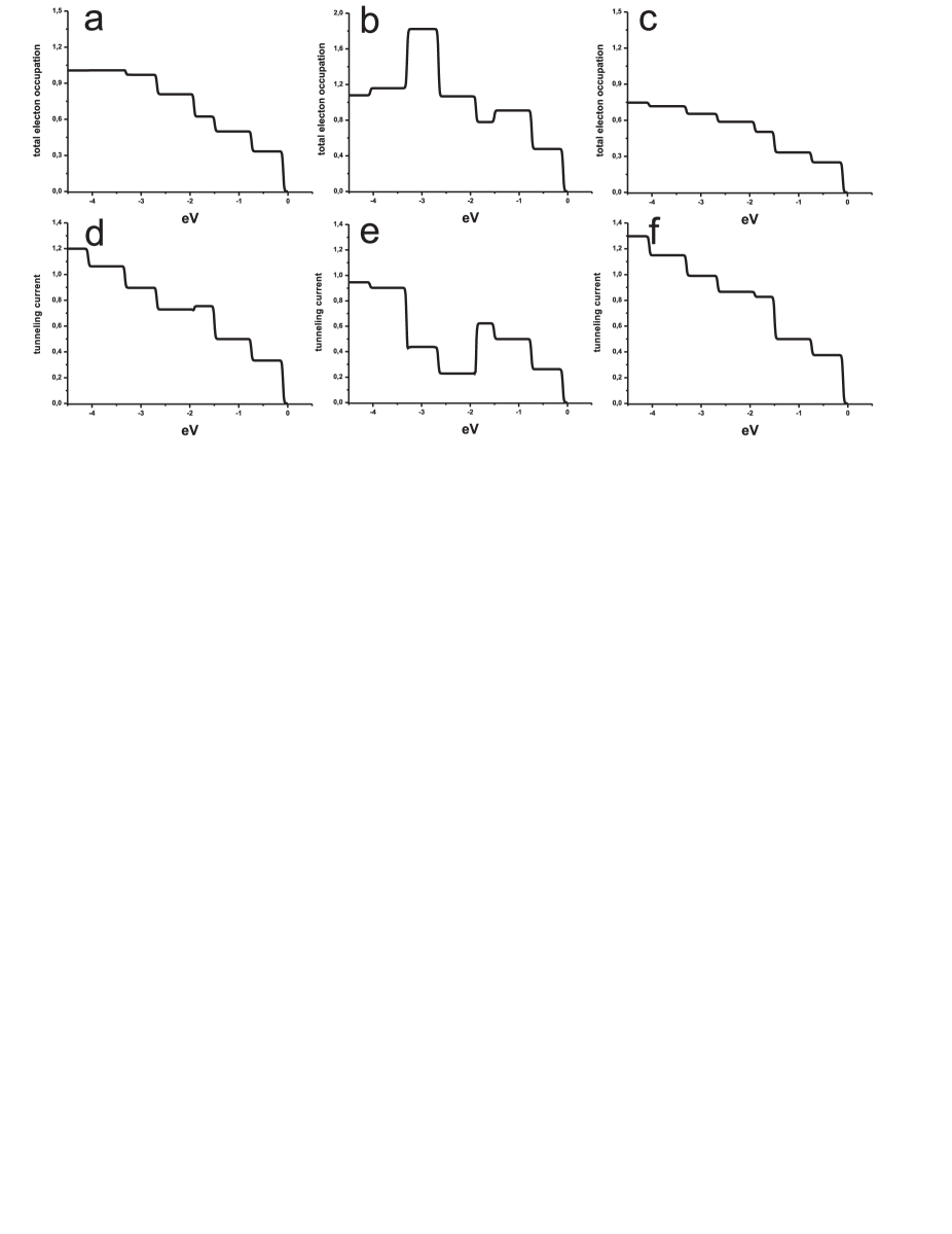
Figure 1: Total electron occupation of the QDs a).-c). and tunneling current d).-f). as a functions of the applied bias voltage for both single electron energy levels located above the sample Fermi level. Parameters $\varepsilon/\Gamma=0.8$, $T/\Gamma=0.7$, $U/\Gamma=1.85$ are the same for all figures. a).,d). $\Gamma_{k}=0.01$, $\Gamma_{p}=0.01$; b).,e). $\Gamma_{k}=0.1$, $\Gamma_{p}=0.01$; c).,f). $\Gamma_{k}=0.01$, $\Gamma_{p}=0.02$.

By means of Heisenberg equations of motion one can get system of equations exactly taking into account correlations of electron filling numbers in localized states in all orders Mantsevich ,Mantsevich_2 (for weak tunneling coupling to the leads). But it is rather tedious to restore the information about the definite charge and spin configurations with different number of electrons from all order correlators for initial levels occupation numbers. So the method based on the pseudo particle operators is more convenient if we are interested in occupation of multi-electron states with particular charge and spin configuration.

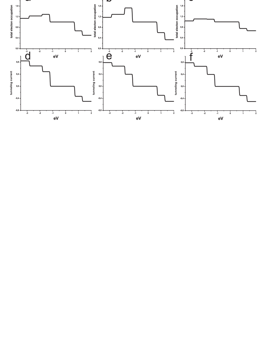
Figure 2: The same dependencies as in the Fig.1 but one single electron energy level is located above and the other - below the sample Fermi level. Parameters $\varepsilon/\Gamma=-0.5$, $T/\Gamma=0.8$, $U/\Gamma=1.5$ are the same for all figures. a).,d). $\Gamma_{k}=0.01$, $\Gamma_{p}=0.01$; b).,e). $\Gamma_{k}=0.02$, $\Gamma_{p}=0.01$; c).,f). $\Gamma_{k}=0.01$, $\Gamma_{p}=0.02$.

III Results and discussion

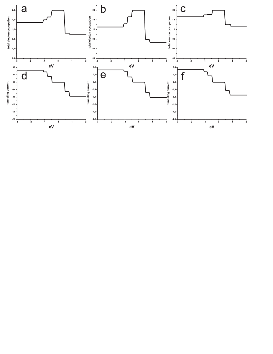
Figure 3: The dependencies of total electron occupation of the QDs a).-c). and tunneling current d).-f). on the applied bias voltage for both single electron energy levels located below the sample Fermi level. Parameters $\varepsilon/\Gamma=-0.5$, $T/\Gamma=0.3$, $U/\Gamma=1.0$ are the same for all cases. a).,d). $\Gamma_{k}=0.01$, $\Gamma_{p}=0.01$; b).,e). $\Gamma_{k}=0.02$, $\Gamma_{p}=0.01$; c).,f). $\Gamma_{k}=0.01$, $\Gamma_{p}=0.02$.

The behavior of the total electron occupation of the coupled QDs $n_{el}(eV)$ and $I-V$ characteristics strongly depends on the parameters of the tunneling contact: energy levels position, the value of the Coulomb interaction and the relation between tunneling rates. The general features of the obtained results is the step-like $I-V$ characteristics with non-equidistant steps related to the energies of the different multi-electron states in the QDs and multiple charge redistribution between the two electron states with different spin configurations (singlet state and triplet state) which appears for the particular range of the system parameters and applied bias voltage.

We first analyze the behavior of the the total electron occupation of the QDs $n_{el}(eV)$ and $I-V$ characteristics of the considered system for different single electron levels positions relative to the sample Fermi level and various tunneling rates to the contact leads (Fig. 1-3). The bias voltage in our calculations is applied to the sample. Consequently, if both single electron levels are above(below) the Fermi level, all the specific features of the total electron occupation and tunneling current characteristics can be observed at negative(positive) values of $eV$. In the case when both single electron energy levels are situated above the sample Fermi level (Fig.1) we observe the step-like behavior of the total electron occupation both for the symmetric ($\Gamma_{k}=\Gamma_{p}$) and asymmetric ($\Gamma_{k}<\Gamma_{p}$) tunneling contact (Fig.1a,c). The width and height of the steps are determined by the relation between the system parameters $T$, $\varepsilon$ and $U$ and $\Gamma=\Gamma_{k}+\Gamma_{p}$.

In the particular range of the applied bias when condition $\Gamma_{k}>\Gamma_{p}$ is fulfilled the total electron occupation demonstrate significant jumps (Fig.1b).

The tunneling current is depicted in Figures 1d-f as a function of the applied bias (tunneling current amplitudes are normalized to $2\frac{\Gamma_{k}\Gamma_{p}}{\Gamma_{k}+\Gamma_{p}}$). In the asymmetric tunneling contact when condition $\Gamma_{k}<\Gamma_{p}$ is valid (Fig.1f) the tunneling current dependence on the applied bias has a step-like structure. In the presence of Coulomb interaction negative tunneling conductivity appears even for symmetric tunneling contact (Fig.1d). The negative differential conductivity is strongly pronounced in the asymmetric tunneling contact when the condition $\Gamma_{k}>\Gamma_{p}$ is fulfilled (Fig.1e).

In a QD without Coulomb interaction the total system occupation can only increase as applied bias increases and passes single electron levels. Quite different situation occurs in a system with strong Coulomb correlations. In the case when one of the single electron energy levels or both of them are situated below the sample Fermi level (Fig.2-3) the total electron occupation of QDs demonstrates pronounced decreasing with increasing of the applied bias (Fig. 2a-c; Fig.3a-c). Equilibrium occupation of two-electron states for zero bias leads to average occupation of one electron per spin (total occupation equal to 2). But when the increasing bias reaches the energies of multi-electron excited states, the total occupation begins to decrease. Using single-electron language we can say that additional tunneling electrons ”push out” electrons from the states below the Fermi level due to Coulomb repulsion. Or one can look at this effect as increasing of probability for electrons to leave the QD due to appearance of several non-elastic channels of tunneling (accompanied with changing of multi-electron states of the QD).

The tunneling current as a function of the applied bias for this case is depicted in Figures 2d-f;3d-f and reveals the monotonic step-like behavior. In both cases the upper single electron energy level ($\varepsilon_{0}+T$) does not appear as a step in the $I-V$ characteristics.

Another interesting feature which appears due to correlations is multiple charge redistribution between the two electron states with different spin configurations (singlet state and triplet state) as a function of the applied bias voltage (Fig.4-6).

In the case of both single electron energy levels situated above the sample Fermi level (Fig.4) several ranges of applied bias exist where the triplet state occupation exceeds the singlet state occupation both for the strong ($U/\Gamma\gg T/\Gamma$) and weak ($U/\Gamma\sim T/\Gamma$) Coulomb interaction. In the case of strong Coulomb interaction localized charge is mostly accumulated in the triplet state.

The occupation of the triplet state with the fixed value of the spin projection $S_{Z}$ is lower than the the occupation of the singlet state if Coulomb repulsion is weak ($U/\Gamma\sim T/\Gamma$) (Fig.4a-c). In the case of strong Coulomb interaction ($U/\Gamma\gg T/\Gamma$) four ranges exist where charge is quite equally distributed between the singlet state and triplet state with the fixed value of the spin projection (Fig.4d,e,f) for different ratios between the tunneling transfer rates.

Figure 5 demonstrates calculation results in the case when one single electron energy level is located above and the other - below the sample Fermi level. For the weak Coulomb interaction ($U/\Gamma\sim T/\Gamma$)the charge is quite completely localized in the singlet state both in the symmetric and asymmetric tunneling contact (Fig.5a-c).

In the case of strong Coulomb interaction ($U/\Gamma\gg T/\Gamma$) charge in the system is also mostly located on the singlet state for the wide range of applied bias (Fig.5d-f), but for some ranges of the applied bias occupation of the triplet state exceeds occupation of the singlet state. But for symmetric tunneling contact the triplet state with the fixed spin projection is always less occupied than the singlet state .

The situation when both single electron energy levels are positioned below the sample Fermi level is demonstrated in Fig.6. In the case of weak Coulomb interaction only one range of the applied bias exists where occupation of the triplet state is equal to or even exceeds the occupation of the singlet state (Fig.6a-c). Occupation of the triplet state with the fixed spin projection is always lower than the occupation of the singlet state. The increasing of the Coulomb interaction leads to the formation of several ranges of the applied bias where triplet state filling numbers exceed singlet state filling numbers (Fig.6d-f).

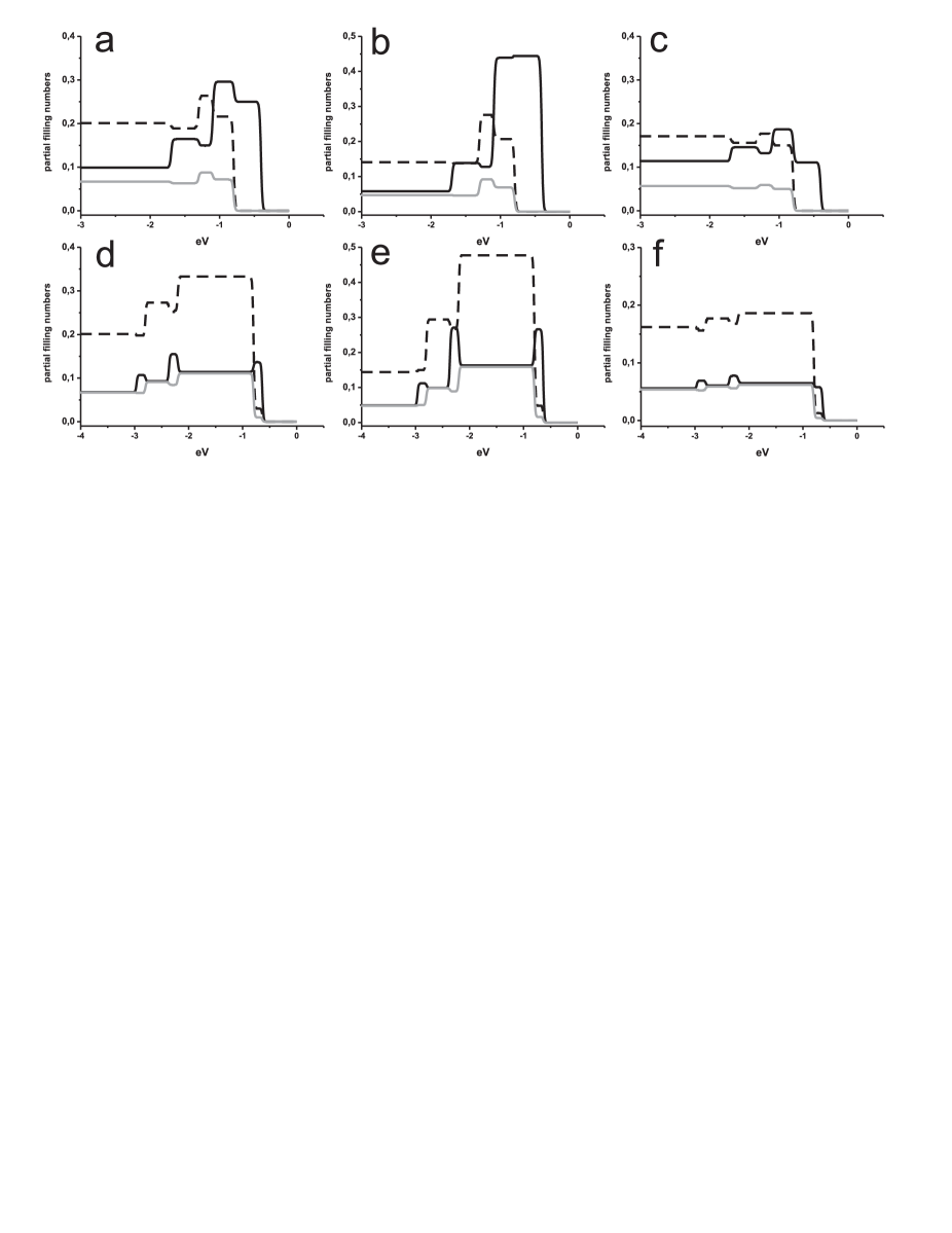
Figure 4: Occupation of two electron state for different spin configurations as a functions of the applied bias voltage for both single electron levels located above the sample Fermi level. Filling numbers in the singlet state are shown by the black line, filling numbers in the triplet state with the fixed projection of the spin are shown by the grey line, full filling numbers in the triplet state are shown by the black-dashed line. Parameters $\varepsilon/\Gamma=0.5$, $T/\Gamma=0.3$ are the same for all figures. a).,d). $\Gamma_{k}=0.01$, $\Gamma_{p}=0.01$; b).,e). $\Gamma_{k}=0.02$, $\Gamma_{p}=0.01$; c).,f). $\Gamma_{k}=0.01$, $\Gamma_{p}=0.02$. a).-c). $U/\Gamma=0.5$; d).-f). $U/\Gamma=2.0$.

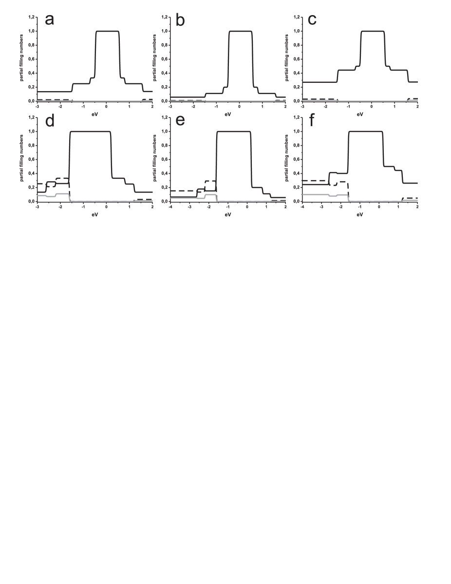
Figure 5: The dependence of two electron state filling numbers for different spin configurations on applied bias voltage when one of the single electron energy levels is located above and the other- below the sample Fermi level. Filling numbers in the singlet state are shown by the black line, filling numbers in the triplet state with the fixed projection of the spin are shown by the grey line, full filling numbers in the triplet state are shown by the black-dashed line. Parameters $\varepsilon/\Gamma=-0.3$, $T/\Gamma=0.5$ are the same for all figures. a).,d). $\Gamma_{k}=0.01$, $\Gamma_{p}=0.01$; b).,e). $\Gamma_{k}=0.02$, $\Gamma_{p}=0.01$; c).,f). $\Gamma_{k}=0.01$, $\Gamma_{p}=0.02$. a).-c). $U/\Gamma=0.5$; d).-f). $U/\Gamma=2.0$.

Figure 6: The same dependencies as on the Fig.4;5 but for both single electron energy levels located below the sample Fermi level. Filling numbers in the singlet state are shown by the black line, filling numbers in the triplet state with the fixed projection of the spin are shown by the grey line, full filling numbers in the triplet state are shown by the black-dashed line. Parameters $\varepsilon/\Gamma=-0.5$, $T/\Gamma=0.3$ are the same for all figures. a).,d). $\Gamma_{k}=0.01$, $\Gamma_{p}=0.01$; b).,e). $\Gamma_{k}=0.02$, $\Gamma_{p}=0.01$; c).,f). $\Gamma_{k}=0.01$, $\Gamma_{p}=0.02$. a).-c). $U/\Gamma=0.5$; d).-f). $U/\Gamma=2.0$.

IV Conclusion

We investigated tunneling through the system of two interacting QDs weakly coupled to the electrodes with Coulomb interaction between localized electrons. In the considered system if electrons number $N$ is changed due to the tunneling processes the modification of the energy spectrum is not reduced to the simple adding of Coulomb interaction $U$ per electron. One, two, three or four electrons can be localized in the coupled QDs , each state with fixed total charge and spin projection has it’s own energy. Transitions between these states were analyzed in terms of pseudo-particle operators with constraint on the possible physical states of the system. Filling numbers of different multi-electron states, total electron occupation of QDs and $I-V$ characteristics were investigated for different single electron levels positions relative to the sample Fermi level and various tunneling transfer rates.

It was shown that total electron occupation demonstrates in some cases significant decreasing with increasing of applied bias - contrary to the situation with no correlations.

We revealed that for some parameter range, the system demonstrates negative tunneling conductivity in certain ranges of the applied bias voltage due to the Coulomb correlations. A negative tunneling conductivity is well pronounced if both energy levels are located above the Fermi level. When energy levels are located on the opposite sites of the Fermi level or both of them are positioned below the Fermi level negative tunneling conductivity was not observed.

Coulomb correlations result in multiple charge redistribution between the two-electron states with different spin configurations (singlet and triplet states) with changing of applied bias voltage. It was found that for particular range of the system parameters the triplet-state occupation can exceed the singlet-state occupation (the inverse occupation takes place).

So tunneling properties of correlated electron systems can be correctly described only in terms of multi-electron states, which allows to find some unexpected effects.

This work was partly supported by the RFBR and Leading Scientific School grants. The support from the Ministry of Science and Education is also acknowledged.

References

• (1) A.N. Vamivakas, C.-Y. Lu, C. Matthiesen et.al., Nature Letters, 467, (2010), 297.
• (2) E.A. Stinaff, M. Scheibner, A.S. Bracker et.al., Science, 311, (2006), 636.
• (3) J.M. Elzerman, K.M. Weiss, J. Miguel-Sanchez et.al., Phys. Rev. Lett., 107, (2011), 017401.
• (4) G. Munoz-Matutano, M. Royo, J.I. Climente et.al., Phys. Rev. B, 84, (2011), 041308(R).
• (5) J. Peng, G. Bester, Phys. Rev. B, 82, (2010), 235314.
• (6) B. Szafran, F.M. Peeters, Phys. Rev. B, 76, (2007), 195442.
• (7) N.S. Wingreen, Y. Meir, Phys. Rev. Lett., 49, (1994), 040.
• (8) S.E. Barnes, J. Phys. F: Met. Phys., 6, (1976), 1375.
• (9) S.E. Barnes, J. Phys. F: Met. Phys., 7, (1977), 2637.
• (10) P. Coleman, Phys. Rev. B, 29, (1984), 3035.
• (11) P. Coleman, Phys. Rev. B, 35, (1987), 5072.
• (12) N. Read, D.M. Newns, J. Phys. C, (1983), 3273.
• (13) N. Read, D.M. Newns, Adv. Phys., 36, (1988), 799.
• (14) N.E. Bickers, Rev. Mod. Phys., 59, (1987), 845.
• (15) P.A. Orellana, G.A. Lara, E.V. Anda, Phys. Rev. B, 65, (2002), 155317.
• (16) J. Paaske, A. Rosch, P. Wolfle, Phys. Rev. B, 69, (2004), 155330.
• (17) J. Paaske, A. Rosch, J. Kroha, P. Wolfle, Phys. Rev. B, 70, (2004), 155301.
• (18) A. Kaminski, Yu. Nazarov, L. Glazman, Phys. Rev. B, 62, (2000), 8154.
• (19) R. Lopez, R. Aguado, G. Platero, Phys. Rev. B, 69, (2004), 235305.
• (20) K. Kikoin, Y. Avishai, Phys. Rev. Lett., 86, (2001), 2090.
• (21) K. Kikoin, Y. Avishai, Phys. Rev. B, 65, (2002), 115329.
• (22) Y. Goldin, Y. Avishai, Phys. Rev. B, 61, (2000), 16750.
• (23) J. Paaske, A. Rosch, J. Kroha et.al, Phys. Rev. B, 70, (2004), 155301.
• (24) P.W. Anderson, Phys. Rev., 164, (1967), 352.
• (25) R. Aguado, D.C. Langreth, Phys. Rev. Lett., 85, (2000), 1946.
• (26) C.A. Busser, E.V. Anda, A.L. Lima et.al., Phys. Rev. B, 62, (2000), 9907.
• (27) P.I. Arseyev, N.S. Maslova, V.N. Mantsevich, JETP, xx, (2012), xx.
• (28) P.I. Arseyev, N.S. Maslova, V.N. Mantsevich, JETP Letters, 94, (2011), 390.