The linewidth-size relationship in the dense ISM of the Central Molecular Zone

Abstract

The linewidth ($\sigma$) – size ($R$) relationship of the interstellar medium (ISM) has been extensively measured and analysed, in both the local ISM and in nearby normal galaxies. Generally, a power-law describes the relationship well with an index ranging from 0.2 – 0.6, and is now referred to as one of “Larson’s Relationships.” The nature of turbulence and star formation is considered to be intimately related to these relationships, so evaluating the $\sigma-R$ correlations in various environments is important for developing a comprehensive understanding of the ISM. We measure the linewidth-size relationship in the Central Molecular Zone (CMZ) of the Galactic Centre using spectral line observations of the high density tracers N₂H⁺, HCN, H¹³CN, and HCO⁺. We construct dendrograms, which map the hierarchical nature of the position-position-velocity (PPV) data, and compute the linewidths and sizes of the dendrogram-defined structures. The dispersions range from $\sim$ 2 – 30 km s^-1 in structures spanning sizes 2 – 40 pc, respectively. By performing Bayesian inference, we show that a power-law with exponent 0.3 – 1.1 can reasonably describe the $\sigma-R$ trend. We demonstrate that the derived $\sigma-R$ relationship is independent of the locations in the PPV dataset where $\sigma$ and $R$ are measured. The uniformity in the $\sigma-R$ relationship indicates that turbulence in the CMZ is driven on the large scales beyond  $\buildrel>\over{\sim}$ 30 pc. We compare the CMZ $\sigma-R$ relationship to that measured in the Galactic molecular cloud Perseus. The exponents between the two systems are similar, suggestive of a connection between the turbulent properties within a cloud to its ambient medium. Yet, the velocity dispersion in the CMZ is systematically higher, resulting in a scaling coefficient that is approximately five times larger. The systematic enhancement of turbulent velocities may be due to the combined effects of increased star formation activity, larger densities, and higher pressures relative to the local ISM.

1 Introduction

Turbulence is observed on all scales larger than the size of the densest star forming cores ($\sim$0.1 pc), and is considered a key process influencing star formation in the interstellar medium (ISM, see Mac Low & Klessen, 2004; McKee & Ostriker, 2007, and references therein). Atomic and molecular line observations provide detailed information about the morphological, thermal, chemical, and dynamical state of the ISM, such as the masses, velocities, and sizes of a variety of structures, from the densest star-forming cores, larger molecular clouds (MCs), and the surrounding, volume filling diffuse gas (e.g. Young & Scoville, 1991; Kalberla & Kerp, 2009; Fukui & Kawamura, 2010, and references therein). Accurately measuring these properties and the relationships between them is necessary for developing a complete understanding of turbulence in the ISM, including its role in the star formation process.

Spectral line observations of the ISM show strong power-law correlations between the mass $M$ and linewidth $\sigma$ with their projected size $R$. Observations of Milky Way MCs generally exhibit exponents $\sim$2 and $\sim$ 0.2 – 0.6 for the mass-size and linewidth-size relationship, respectively (Larson, 1981; Solomon et al., 1987; Leisawitz, 1990; Falgarone et al., 1992; Caselli & Myers, 1995; Kauffmann et al., 2010a, b; Beaumont et al., 2012). Similar trends are observed for extragalactic clouds (Bolatto et al., 2008; Sheth et al., 2008). These results are interpreted as evidence that MCs are virialized objects, and are generally referred to as “Larson’s Relationships.”

That the $M-R$ and $\sigma-R$ relationships portray similar power law scalings across a range in environments suggests that the underlying physical processes driving ISM dynamics is “universal” (e.g. Heyer & Brunt, 2004). However, it is not clear if this “universality” applies to systems significantly different than the Milky Way or Local Group GMCs, as it has not been possible to sufficiently resolve the ISM in external systems. Measuring these relationships in varying environments, such as (ultra) luminous infrared galaxies ([U]LIRGs) or similar starbursting regions like the Galactic Centre, is required to comprehensively understand the ISM throughout the universe.

To understand the nature of turbulence in a starbursting environment, we investigate the linewidth-size relationship of high density structures in the Central Molecular Zone (CMZ) of the Galactic Centre (GC). The CMZ is denser than the ISM outside the GC, with densities comparable to the star forming cores within MCs (see Morris & Serabyn, 1996, and references therein). The star formation rate in the CMZ is $\sim$1.5 orders of magnitude higher than the rate measured in the solar neighborhood (Yusef-Zadeh et al., 2009). Therefore, the star formation activity in the GC is in many ways similar to starbursting systems like LIRGs. Given its relatively close proximity ($\sim$ 8 kpc), the GC affords us the best opportunity to resolve the structure of the ISM in starbursting environments, and probe the nature of the dynamic ISM.

In this work, we measure the linewidth-size relationship in the CMZ using Mopra observations of dense gas tracers. Miyazaki & Tsuboi (2000) and Oka et al. (1998, 2001) present an analysis of the Larson scaling relationships from Nobeyama observations of CS and ¹²CO, respectively. They show that the $\sigma-R$ relationship in the CMZ is similar to that in the Milky Way disk, but with enhanced velocities. We extend their analysis by considering four high density tracers, N₂H⁺ and H¹³CN with low opacity, as well as HCN and HCO⁺ with high opacity. Further, the Mopra coverage of the CMZ is fully (Nyquist) sampled, allowing for thorough and systematic identification of dense clouds. By constructing hierarchical structure trees, or dendrograms (Rosolowsky et al., 2008), we identify contiguous features in the observed position-position-velocity (PPV) cubes of the CMZ. One key difference between our study and previous efforts is the manner in which “clouds” are identified. Dendrograms map the full hierarchy of structures, such that ISM structures which are not necessarily part of the densest clouds are included in our analysis. We assess the linewidth-size relationship of the ensemble of these structures, and compare it to the well known $\sigma-R$ trends found in the local ISM.

This paper is organised as follows. The next section describes the observations of high density tracers in the CMZ. In Section 2.3, we describe the method we use to identify contiguous structures in the observed data. Section 3 presents the linewidth-size relationship. In Section 4 we discuss how the measured $\sigma-R$ relationship relates to the underlying turbulent velocity field, and compare it to the trend in the Milky Way molecular cloud Perseus. We summarise our findings in Section 5.

2 Observations and Analysis Technique

2.1 Mopra survey of the CMZ

In our analysis of the linewidth-size relationship of the CMZ, we use the observations from the 22 metre Mopra millimetre-wave telescope, which is operated by the Australia Telescope National Facility (ATNF). The Mopra CMZ survey covers the 85-93 GHz window, covering 20 spectral lines including a number of dense gas tracers like the HCN, HNC and HCO⁺ molecules, as well as the cold core species N₂H⁺ (Jones et al., 2012). The total area covered by the survey is 2.5$\times$0.5 deg², with 40″ spatial resolution ($\sim$2 pc at a distance of 8 kpc), and spectral resolution $<$ 0.9 km s^-1. For our analysis, we use smoothed datasets with 3.6 km s^-1 spectral resolution of observations of the lowest rotational transitions of four molecules: N₂H⁺ (rest frequency 93.173 GHz), HCN (88.632 GHz), H¹³CN (86.340 GHz), and HCO⁺ (89.189 GHz). Further information about the Mopra CMZ survey, including reduction techniques, intensity maps, and velocity structure, is described in Jones et al. (2012).

2.2 ¹³CO FCRAO observations of the Perseus molecular cloud

In Section 4.4, we compare the linewidth-size relationships in the CMZ to the Milky Way molecular cloud Perseus. We use the ¹³CO J=1–0 line (110.201 GHz) data from the COMPLETE Survey (Ridge et al., 2006). The data are approximately Nyquist sampled, with a pixel size of 23″ (.028 pc at a distance of 250 pc), and have a velocity resolution of 0.066 km s^-1. Ridge et al. (2006) describes the COMPLETE observations of Perseus, including ¹²CO and ¹³CO, as well as HI, dust extinction and emission maps of the cloud.

2.3 Measuring the linewidth-size relationship

In order to measure the linewidth and sizes of structures, we first need to identify the relevant structures using a well defined criterion. One rather simple definition of a structure is any contiguous region with (approximately) constant density. Unfortunately, we only have information about the intensity of a number of spectral lines at a range of velocities, along lines of sight (LoS) through the CMZ. As the CMZ has extremely dense structure throughout its volume, velocity integrated intensity maps would merge a number of dense features along the LoS, thereby smoothing out the intrinsic structure of the ISM in the resulting 2-dimensional (2D) map (e.g. Pichardo et al., 2000; Ballesteros-Paredes & Mac Low, 2002; Gammie et al., 2003; Shetty et al., 2010). Accordingly, contiguous regions in the 3-dimensional (3D) PPV space should be able to more accurately identify distinct structures. As the ISM contains hierarchical structure, direct clump decomposition methods may not accurately identify different levels of substructure, especially in high density, turbulent environments. We thus employ the dendrogram decomposition technique (Rosolowsky et al., 2008) to identify and characterize contiguous structures from the PPV cubes of the CMZ.

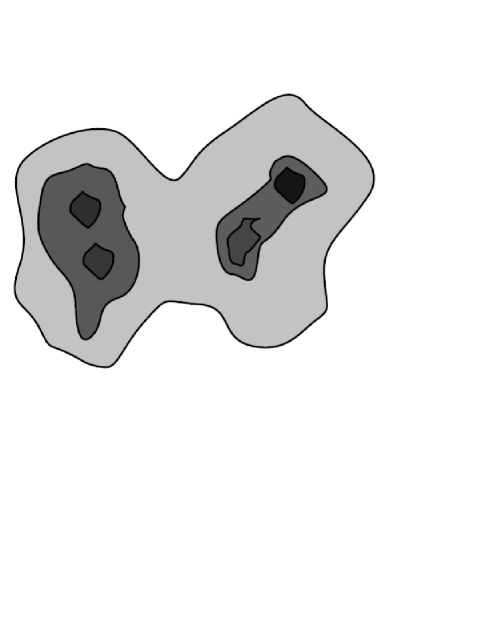
Figure 1: Dendrogram of a hierarchical cloud. Left: simple cloud with three levels of hierarchical substructure. Right: Dendrogram, or structure tree, of the cloud. Each distinct (closed contour) region, is identified as a structure (vertical lines). Structures on the top of the tree are “leaves.” The structures which enclose multiple higher level contours are “branches,” and the structure which encloses all other structures is a “root.”

We provide a brief overview of dendrograms here, and refer the reader to Rosolowsky et al. (2008) for a more detailed description of the structure decomposition algorithm. Dendrograms provide a “structure tree” which quantifies the hierarchical nature of any dataset. Consider the cloud depicted in Figure 1. The cloud is composed of three different levels, or intensities, with the base level (light blue structure) enclosing all higher levels. Each structure at a given level is distinguishable from adjacent structures if a closed iso-intensity contour can enclose the whole structure. As the intensities of the features do not merge in a contiguous manner, they are identified as separate structures. Both structures in the second level encloses higher intensity regions, which are themselves separated into two distinct structures.

The structure tree in Figure 1 maps the hierarchical nature of the model cloud. Each vertical line corresponds to a distinct structure in the cloud. Those on the top of the tree are referred to as “leaves.” The lowest level is the “root” of the tree. Any level which encloses multiple structures requires “branches” to accommodate the hierarchy. The leaves at top of the tree shows the highest density structures which do not enclose any further substructure.

The mapping illustrated in Figure 1 can also be performed for 3D data, such as a PPV cube. Each structure corresponds to an iso-intensity region in PPV space. Additional information can be derived from the dendrogram-identified regions. As the structures from a PPV cube demarcate iso-intensity regions, the velocity dispersions $\sigma$ of this structure may be directly computed. We compute the intensity weighted velocity dispersion of each structure

$$\sigma=\left[\frac{\sum{I_{v}(v-\bar{v})^{2}}}{\sum{I_{v}}}\right]^{\frac{1}{2}},$$ (1)

where the summations are taken over all zones of the identified structures, $I_{v}$ is the line intensity, $v$ is the LoS velocity, and and $\bar{v}$ is the intensity weighted mean velocity, $\sum(I_{v}v)/\sum I_{v}$. We also define the size $R$ of each structure using the projected area, $R=(N_{\rm proj}\Delta x\Delta y/\pi)^{\frac{1}{2}}$, where $N_{\rm proj}$ is the number of projected pixels, and $\Delta x\Delta y$ is the area of the resolution element.

To ensure that the dendrogram defined structures are well resolved, we exclude any features with $R<2$ pc, and $\sigma<2$ km s^-1. Since we are interested in the dispersion of the contiguous and distinct structures, and not the whole ISM in the CMZ, we also only consider features with $R<40$ pc. Such a size limit may further minimise contamination from the superposition of features along the LoS. Finally, we also exclude any region which occurs within three voxels (zones in a PPV dataset) from the boundary of the PPV cubes. Under these conditions, we minimise the likelihood of identifying features dominated by observational noise, resulting in well defined and contiguous structures PPV space. We have adopted a uniform “dendrogramming” strategy such that each structure contains at least 50 voxels. This condition ensures that the dendrogram identifies real extended structures in the PPV cube, which are unlikely to be purely noisy features. From the measured value of $\sigma$ and $R$, we can now assess the linewidth-size relationship of the ensemble of dendrogram defined structures.

Figure 2: Linewidth-size relationship in the CMZ, as measured within dendrogram identified structures in N₂H⁺, HCN, H¹³CN, and HCO⁺. Filled symbols correspond to “leaves” which do not enclose additional higher level structures. Open symbols are structures which do contain higher level structures. Lines show the best ($\chi^{2}$) power-law fits.

3 The linewidth-size relationship in the CMZ

Figure 2 shows the $\sigma-R$ relationship of the dendrogram defined structures from the N₂H⁺, HCN, H¹³CN, and HCO⁺ observations of the CMZ. The largest structures identified in each tracer all have dispersions of 20–30 km s^-1, which is equivalent to the global linewidth of the CMZ. These structures generally enclose higher level, brighter features. Towards smaller scales, the dispersions systematically decrease, reaching $\sim$2 km s^-1 in structures with $R$$\sim$2 pc. The open symbols in Figure 2 are regions which contain at least one higher level structure. The closed symbols correspond to the leaves on the top of the structure tree (see Fig 1). The ensemble of structures exhibit a systematic decrease in linewidths from the largest scale structures to the smallest, brightest features in all the observed lines.

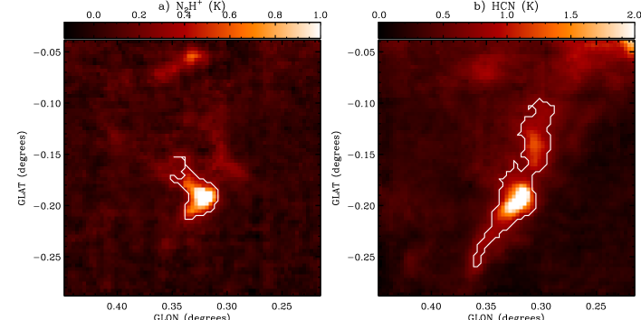
Figure 3: A single a) N₂H⁺ and b) HCN channel map (corresponding to velocity $V_{\rm LSR}\sim$140 km s^-1) showing a dense filamentary region near to the Galactic Centre. White contours show the cross-section of one dendrogram defined iso-intensity surface at this velocity. The linewidths and sizes of the whole dendrogram structures are 2.8 km s^-1 and 2.8 pc in N₂H⁺, and 2.1 km s^-1 and 5.1 pc in HCN, respectively.

That the structures in all tracers span a limited region in $\sigma-R$ space, as well as depict similar trends, provides confidence that the apparent $\sigma-R$ relationship in Figure 2 is real. N₂H⁺ has a critical density of $\sim$$10^{5}$ cm^-3, and is a good tracer of cold, dense cores. HCN and HCO⁺ traces more extended dense gas in the ISM (see Figure 2 in Jones et al. 2012), with similar critical densities for each $J$=1-0 emission lines. They can be moderately optically thick in the CMZ, as analysed by Jones et al. (2012). Hence, we perform the analysis on the weaker, but optically thin H¹³CN line, obtaining essentially the same results; this indicates that optical depth has not significantly biased the trends. Both HCN and N₂H⁺ exhibit hyperfine splitting, being split over $\sim$14 km s^-1 into 3 groups of lines in the ratio 3:5:1. Though this is less than the typical turbulent width for the gas in the CMZ, multiple smaller scale dendrogram structures in N₂H⁺ and HCN may actually be part of a single feature. On the other hand HCO⁺, which is not split into any sub-components, produces very similar results, indicating that the derived linewidth-size relation of the ensemble is not significantly affected by line splitting.

There are some differences between the linewidth-size trends from the various tracers shown in Figure 2. Most notably, the HCN and HCO⁺ have a number of larger scale structures with $R$  $\buildrel>\over{\sim}$ 3 pc and $\sigma$ $\buildrel<\over{\sim}$ 5 km s^-1 that do not occur in N₂H⁺. These differences can be largely attributed to the relative extents of the different tracers, and for some structures the foreground absorption of HCN and HCO⁺ emission.

For some of the large $R$ and low $\sigma$ points, a closer inspection of these structures reveals that they are further divided into separate features in the N₂H⁺ dataset. Figure 3 shows an example of one such structure in N₂H⁺ and HCN. The HCN dendrogram-defined contour corresponds to the leaf with the lowest $\sigma$= 2.1 km s^-1, with $R$= 5.1 pc. The dendrogram of the N₂H⁺ feature, on the other hand, is more compact with $R$= 2.8 pc and $\sigma$= 2.8 km s^-1. N₂H⁺ traces cold, dense cores, and as it can be destroyed by reactions with CO, it is expected to be present in the densest and most quiescent regions where CO is depleted (see Bergin & Tafalla, 2007, and references therein). N₂H⁺ is also found to be less extended than HCN and HCO⁺ (Purcell et al., 2006, 2009). In addition, the HCN and HCO⁺ line emission has higher optical depth. Hence the dendrogram of an HCN and HCO⁺ structure may therefore demarcate a larger region surrounding a dense peak than does N₂H⁺, as shown in Figure 3. Consequently, an extended HCN structure may be found to break up into a number of compact N₂H⁺ features, with similar measured linewidths. The discrepancies in the $\sigma$ and $R$ provided by the different tracers may not necessarily reflect morphological variations of the gas, but rather diversity in chemical abundances. The subdivision of features in the N₂H⁺ observations results in a more uniform $\sigma-R$ relationship, and correspondingly a better defined trend for a larger range in sizes.

As discussed by Jones et al. (2012), there are strong foreground absorption features in the HCN and HCO⁺ datasets, possibly due to the presence of the spiral arms along the LoS. The sharp drop in intensity of some of the large scale features across the velocity channels corresponding to -52, -28, and -3 km s^-1 leads the dendrogram algorithm to identify multiple structures. Consequently, such an extended feature only spans a limited range in velocity, thereby resulting in a structure with large $R$ but low $\sigma$. The division of large scale structures due to foreground absorption along the LoS does not occur as much in N₂H⁺ and H¹³CN, as those molecules are not as pervasive, resulting in substructure that can be more easily differentiated from its background, as described above.

The $\sigma-R$ trends shown in Figure 2 indicate that there is a large range of possible dispersions for a given size, reaching  $\buildrel>\over{\sim}$ 7 km s^-1 in the HCN dataset. Several factors can affect the amount of substructure and measured properties from any observation, including signal-to-noise ratio, resolution, chemical abundance inhomogeneities, and radiative transfer effects (opacity, sensitivity to temperature and density). Further, local systematic effects may influence some regions of the ISM more than others. For instance, Rodriguez-Fernandez & Combes (2008) suggest that infalling gas along spiral arms and through the large cloud complex at longitude 1.3^o lead to the asymmetry of the CMZ. We find that the measured linewidths in this region are not particularly discrepant from the ensemble, as the values of $\sigma$ and $R$ measured in that complex fall within the range provided by the other structures. The intrinsic scatter of the measured $\sigma$ for structures with similar sizes may be reflective of the differences in environmental conditions across the ISM.

Despite the numerous physical processes that likely influence the gas dynamics in the CMZ, Figure 2 shows that the linewidths are correlated with the sizes. The Pearson’s correlation coefficient of the N₂H⁺, HCN, H¹³CN, and HCO⁺ linwidth-size data (in log space) are 0.84, 0.58, 0.86, and 0.72, respectively. The ensemble may thereby be described as power-law relationships. To quantify the power-law, we fit

$$\left(\frac{\sigma}{\rm km\,s^{-1}}\right)=A\left(\frac{R}{\rm pc}\right)^{b}$$ (2)

in log space to the dendrogram derived linewidths and sizes. The fit estimates the power law index $b$ and coefficient $A$. We first employ a $\chi^{2}$ fit, and in order to comprehensively account for the uncertainties, we also perform a Bayesian linear regression analysis.

3.1 Least squares ($\chi^{2}$) fit

As a first estimate of the power-law index and coefficient, we apply a standard $\chi^{2}$ fit. Each panel in Figure 2 shows the $\chi^{2}$ fit lines, and Table 1 provides the best fit parameters. The maximum error in the best fit slopes is 0.06, obtained from the HCO⁺ structures. This error is the formal $\chi^{2}$ error, and in this case is primarily driven by the large number of points which results in rather low values. The resulting error estimates suggest that to a high degree of probability (3$\sigma$) the N₂H⁺ and HCN features have different slopes. In principle, it is possible that different molecules exhibit different $\sigma-R$ slopes, since they may span different regions in the ISM. Such disparity may be expected when considering tracers of different densities (e.g. ¹²CO vs. HCN), which would correspond to regions with variable extents. However, in this study we are focusing only on high density tracers, and a direct comparison of the structures in the PPV datacubes do not show obvious signs that the tracers span regions of variable spatial extents. Additionally, Figure 2 suggests significant overlap of $\sigma$ and $R$ for each of the tracers. Therefore, the low error estimate in the $\chi^{2}$ fit may not accurately characterize the uncertainty in the linewidth-size relationship. In order to rigorously account for the errors, as well as ascertain the full range of possible best fit parameters, we employ a Monte Carlo analysis and a Bayesian linear regression fit for estimating the coefficient and power-law index.

Table 1: Best ($\chi^{2}$) fit parameters of linewidth-size relationship¹

Tracer	N2H+	HCN	H13CN	HCO+
Power law index $b$	0.67	0.46	0.78	0.64
Coefficient $A$	2.6	3.8	2.6	2.1

3.2 Uncertainties in the dendrograms

Dendrograms identify contiguous structures in the PPV cubes based on the intensity at each position and LoS velocity. Any uncertainties in the intensities may lead to inaccurate identification of structures, and thereby an erroneous $\sigma-R$ relationship. To assess the magnitude of these uncertainties, we perform a simple bootstrapping analysis.

For this analysis we use the N₂H⁺ dataset, which has a well defined $\sigma-R$ relationship. We estimate a 1$\sigma$ uncertainty 0.04 K from a region far from any significant emission. For each realization in the Monte Carlo simulation, we modify each voxel in the PPV cube by an additive factor $\epsilon$, where $\epsilon$ is drawn from a normal distribution with 0 mean and 0.04 K standard deviation. After constructing the structure tree, we fit the linewidths and sizes as described above.

After performing this exercise 100 times, we measure a standard deviation in the best fit parameters $b$ and $A$ to be  $\buildrel<\over{\sim}$ 0.01. This value is lower than the errors returned by the $\chi^{2}$ fit of the original unperturbed dataset. This test indicates that the variance in the number of structures, as well as the uncertainty in the estimated linewidths and sizes due to noise, hardly influences the fit $\sigma-R$ relationship. We have performed a similar analysis on the other three datasets, and as with the N₂H⁺ analysis, we find that the range in the best fit parameters to be smaller than the errors computed in the $\chi^{2}$ fit. We can thus be confident that the dendrograms of the original dataset are not sensitive to noise in the PPV datacubes. We now turn our attention to the affect of resolution, for which we employ a Bayesian linear regression analysis.

3.3 Bayesian regression fit

One of the primary advantages of Bayesian inference is that the uncertainties in the measured data are rigorously and self-consistently treated (e.g. Gelman et al., 2004; Kruschke, 2011). A Bayesian fit considers the error in each measured quantity, in our case $\sigma$ and $R$, to be drawn from some a priori defined distribution. The choice of the distribution should reflect the uncertainties in the measurement. Commonly, Bayesian inference utilizes Markov Chain Monte Carlo (MCMC) routines to sample the probability distribution of the fit parameters, given the measured data and the assumed uncertainties. The result of the Bayesian inference is a joint probability $-$ or posterior $-$ distribution of the regression parameters. This probability distribution function (PDF) accounts for the assumed measurement error distributions, and therefore provides well defined uncertainty estimates on each of the fit parameters, as well as the correlations between them. We refer the reader to Kelly (2007) for details of the Bayesian fitting algorithm we use in our analysis.

For our estimate on the uncertainties in the size we use the effective spatial resolution of the observational datasets. For the error estimate in the velocity dispersion, we choose a conservative value of 2 km s^-1, which is about twice the resolution of the original observations. Note that though the resolution of the smoothed datacube (3.6 km s^-1) is larger, any given contiguous region in a PPV cube may produce a dispersion lower than the effective resolution, as the dispersion is simply a measure of the deviation from the mean value. The smoothing primarily affects the very smallest features with narrow lines, which are excluded from our analysis given our criteria described in Section 2.3.

In deriving the linewidths and sizes, we extract contiguous regions in PPV space defined by the dendrogram algorithm. Though this process introduces additional sources of error, we have shown in Section 3.2 that these uncertainties are minimal, and hardly affect the $\sigma-R$ relationship. Therefore, in our Bayesian fit we only consider the uncertainties due to resolution (e.g. beam smearing). We are thus effectively assuming that resolution is the dominant source of uncertainty, and that the errors in log($\sigma$) and log($R$) are normally distributed, with dispersions 2 km s^-1 and 2 pc, respectively.

Figure 4 shows the Bayesian fit of the N₂H⁺ $\sigma-R$ relationship. The peak of the posterior, corresponding to $\sigma=2.2R^{0.78}$, is shown as the blue line. As expected, this line is similar to the $\chi^{2}$ fit. The gray lines in Figure 4 are five random draws from the Bayesian posterior. The inset plot shows the marginal probability distribution of $b$. The 95% (2$\sigma$) highest density interval, or HDI, is marked by the vertical dashed lines, $b\in$ 0.41 $-$1.13. This HDI provides a quantitative prediction of the range in possible $b$, given the uncertainties in the measurements of $\sigma$ and $R$. The distribution of $b$ inferred by the Bayesian fit is six times larger than the uncertainty in the $\chi^{2}$ estimate.

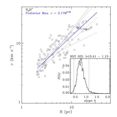
Figure 4: Bayesian regression of linewidth-size relationship in N₂H⁺ structures. Open circles are the dendrogram derived linewidths and sizes. The blue line corresponds to the fit with the highest probability. The gray lines show five random draws from the Bayesian posterior. The inset shows the marginal probability distribution $P(b)$ of the power-law index. Vertical dashed lines indicate the 95% highest density interval (HDI), which ranges from 0.41 $-$ 1.13.

Figure 5 provides the marginal PDFs of the fit indices for all four tracers. The H¹³CN PDF is noticeably wider, reflective of the lower number of identified structures in that tracer (Fig. 2). Table 2 indicates the parameters from the peak of the posterior and in the 95% HDI for all the tracers. There is substantial overlap between the PDFs from the different tracers, in both the coefficient and the exponent. It is common practice in Bayesian inference to consider the full 95% HDI as the reasonable range of fit parameters, rather than any single “best-fit” point estimate, so that the measurement uncertainties are taken into account. Under this framework, we cannot conclude that the evidence suggests a different $\sigma-R$ relationship for the various tracers.

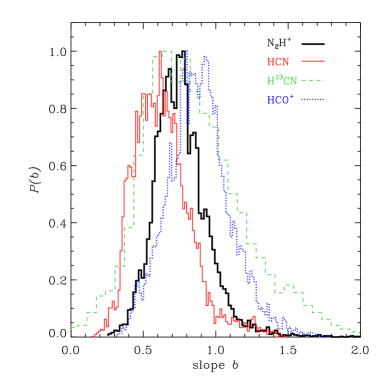
Figure 5: Marginal distributions of the index $b$ from the Bayesian regression analysis of the $\sigma-R$ relationship from N₂H⁺ (thick black), HCN (thin red), H¹³CN (dashed green), and HCO⁺ (dotted blue). Table 2 provides the mode and the 95% highest density intervals of these PDFs.

Table 2: Results from Bayesian inference of linewidth-size parameters

Tracer	N2H+	HCN	H13CN	HCO+
Highest probability for $b$	0.78	0.62	0.66	0.79
95% HDI of $b$	0.41$-$1.13	0.27$-$1.02	0.21$-$1.66	0.45$-$1.30
Highest probability for $A$	2.2	2.7	2.9	1.7
95% HDI of $A$	0.9$-$3.8	1.1$-$4.7	0.0$-$5.8	0.5$-$2.7

4 Discussion

4.1 Do the growth of structures affect the $\sigma-R$ relationship?

The uniform $\sigma-R$ trend over the full range in spatial scale shown in Figure 2 suggests some connection between the densest structures and the larger scale ISM in the GC. As we discuss further in Section 4.4, this trend is also observed for clouds in the Milky Way disk, and provides evidence for large-scale turbulent driving. One closely related question is whether the growth of dense structures within a turbulent medium influences the underlying velocity field.

To investigate the impact of dense clouds on the linewidth-size relationship, we perform a similar analysis to that described in Section 2.3, but with a few modifications. First, we assess the role of intensity weighting, simply by excluding the weighting factor $I_{v}$ in Equation 1. Next, we also measure the linewidth in random locations in the PPV cubes, using the dendrogram defined contours placed at different locations throughout the PPV cubes. For the latter exercise, we shift the contours to a different random location, such that the contours no longer demarcate iso-intensity surfaces. As a result, the shape of the contour is preserved, but the PPV region within the shifted contour may consist of a number of dense complexes, diffuse gas, or some combination of both. To ensure that results are statistically robust, we perform numerous realizations of this exercise. Through these modified analyses, we can investigate the extent which the growth of dense structures and their internal processes influences the $\sigma-R$ relationship.

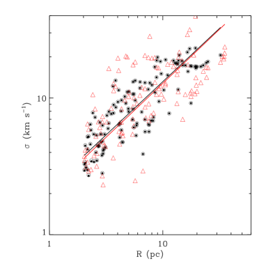
Figure 6: Linewidth-size relationship of the N₂H⁺ points. Black open circles are the original N₂H⁺ measurements, and the black line is the most probable Bayesian inferred fit $\sigma=2.2R^{0.78}$. Black solid circles show the linewidths computed without any intensity weighting. Red triangles are the measurements from random locations in the PPV cube, using dendrogram defined contours. The red line is the most probable Bayesian inferred fit, $\sigma=2.1R^{0.79}$.

Figure 6 shows the results from this modified analysis. The open circles are the original intensity weighted N₂H⁺ $\sigma-R$ points, and the solid line shows the fit derived from the maximum of the Bayesian posterior discussed previously and presented in Figure 4. The smaller solid circles are the measurements where there is no intensity weighting. There is almost no difference between these two sets of points, since the intensity range within a given structure is limited.

The red open triangles in Figure 6 show the results of one realization where the original dendrogram contours have been randomly shifted to a different PPV location. For this particular realization, the contours have been shifted by a minimum of 50 voxels in each of the three dimensions of the PPV cube, plus an additional random value drawn from a uniform distribution between 0 and 20. There is still a clear trend of increasing linewidth with increasing size, with slightly more scatter than the original $\sigma-R$ distribution. The solid red line shows $\sigma=2.1R^{0.79}$, which corresponds to the maximum of the Bayesian posterior for this dataset. This result is very similar to the original N₂H⁺relationship, and the HDIs for the two PDFs almost completely overlap. We have performed ten different realizations of such a random shifting of the dendrogram contours, varying the amount by which the contours are shifted, and each one produces very similar results which are statistically indistinguishable from the original N₂H⁺ relationship. We have also performed this analysis on the HCN, HCO⁺, and H¹³CN datasets, and find the resulting $\sigma-R$ relationships to be statistically indistinguishable from the corresponding original results.

As clouds begin to grow, self-gravity and other internal process will begin to play a role in their subsequent dynamics. If internal processes dominate the ensuing dynamics of the clouds, we should find a distinct difference between the $\sigma-R$ computed from the dense structures, and that measured from random regions irrespective of the presence of dense structures. That the measured $\sigma-R$ relationship can be reproduced regardless of the precise locations (in PPV space) where the linewidths are measured indicates that the dense cloud dynamics is predominantly governed by the underlying turbulent flow, with little contribution from internal sources of turbulence.

In fact, a very similar analysis was carried out by Issa et al. (1990), who concluded that the interpretation by Solomon et al. (1987) that GMCs are bound arises due to the spatial and spectral crowding of clouds, in combination with the method employed to identify clouds in PPV cubes. Our analysis is in agreement with Issa et al. (1990). The measured $\sigma-R$ relationship cannot fully reveal the dynamical state of the dense clouds. These results indicate that turbulence within dense clouds are driven on the largest scales in the ISM, a topic we further discuss in Section 4.4.

Besides revealing that turbulence must be driven on the largest scales, the measured $\sigma-R$ relationships may delineate a lower limit to the turbulent driving scale. Applying different statistical tools on numerical simulations, such as structure functions and $\Delta$-variance, Ossenkopf & Mac Low (2002) showed that beyond the driving scale $\sigma$ will remain nearly constant with increasing $R$. Moreover, dendrograms are capable of identifying the flattening of the linewidth-size relationship towards the scales at which turbulence is injected, as shown by Shetty et al. (2010) and Shetty et al. (2011, see their Fig. 13) using numerical simulations. Although the N₂H⁺, HCN, and HCO⁺ $\sigma-R$ pairs show some semblance of a decrease in $b$ at the largest scales (Fig. 2), there is no strong evidence for such flattening. Since $\sigma$ increases with $R$ up to the largest scales in our analysis, we conclude that turbulence in the CMZ is predominantly driven on scales  $\buildrel>\over{\sim}$ 30 pc. Note that though turbulence is driven on the large scales, it produces a velocity field which must be coherent on much smaller scales. Quantifying this coherence may further reveal additional properties of the turbulent ISM.

4.2 The relationship between the shape of dense structures and the $\sigma-R$ relationship

So far, we have defined the contiguous structures in PPV space via dendrograms. That is, their shapes are governed by the morphology and velocity extent of the structures in the ISM. In the analysis described above, we have shown that the measured linewidths are rather insensitive to the location in PPV space where they are measured. We now consider whether the precise shape of the defined structures affect the linewidth measurement by analysing regions with arbitrary shapes. We consider two simple cases, one in which the linewidths are measured in spherical regions, and one using cubic regions from the PPV cube.

Figure 7 shows the result of this exercise, comparing the spherical and cubic derived linewidths to a representation of the original dendrogram derived relationship from the N₂H⁺ observations. To portray the original measurement, we employ a “posterior prediction” from the Bayesian regression of the N₂H⁺ dataset shown in Figure 4. Posterior prediction is a straightforward way of comparing the Bayesian fit with new data. In other words, it can “predict” new (or future) measurements based on the model derived from the existing data (see e.g. Gelman et al., 2004; Kruschke, 2011). From the Bayesian posterior, at each MCMC step we can draw a large sample of $\sigma$ for chosen values of $R$. Due to the uncertainties and the dispersion about the regression line, the posterior defines a range in possible $\sigma$ values. The 95% HDI of the predicted $\sigma$ values from the dendrogram derived $\sigma-R$ relationship is shown by the green lines in Figure 7, and the short horizontal lines show the mean value. Subsequent data that fall within the extent of the vertical lines are considered to be consistent with the Bayesian inferred $\sigma-R$ relationship.

The blue circles in Figure 7 show the measured linewidths in randomly extracted spherical regions in the N₂H⁺ PPV cube. The sizes of the spheres are determined by the chosen value of the radius. There are up to three spheres for each size considered, but as the measured linewidths of each one are nearly identical, it is difficult to distinguish the multiple structures. The red squares are measurements extracted from cubic regions. The sizes $R$ of the squares are computed in the same manner used to define the sizes of the dendrogram structures, $R=\sqrt{{\rm A}/\pi}=L/\sqrt{\pi}$, where $L$ is the length of one side of a face of the cube lying on the 2D plane spanning the spatial dimensions of the PPV cube. The extent of the spheres and cubes along the velocity dimension of the PPV cube is rather arbitrarily chosen. The measured velocity dispersion simply scales with the velocity extent over which it is measured. For the cubes considered in Figure 7, we simply set the extent in the number of channels to be equal to the number of spatial pixels defining the cube. Similarly, for the sphere the number of spatial pixels defining the “radius” sets the extent in velocity. Had we increased the extent in velocity, the cube would instead be a cuboid (a 3D rectangle), and the sphere would be a cylindrical region oriented parallel to the velocity axis, with semi-spherical ends. Yet, the size would remain the same, due to its working definition. Clearly, for the cubes and spheres in Figure 7 as we have defined them the measured linewidths are dependent on the spectral resolution of the dataset.

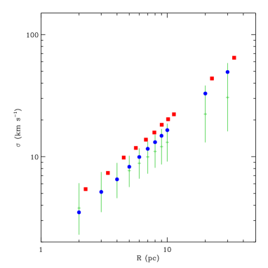
Figure 7: Linewidth-size relationship of spherical (blue circles) and cubic (red squares) regions measured in the N₂H⁺ PPV dataset. For comparison, the horizontal green dashes are the predicted mean values of $\sigma$ from the Bayesian posterior (see Fig. 4). The green vertical lines show the 95% HDI of the predicted values of $\sigma$ for each $R$.

In general, the precise manner in which the sizes are defined will affect any inferred $\sigma-R$ relationship, as discussed previously by Ballesteros-Paredes & Mac Low (2002) and Shetty et al. (2010). Therefore, such caveats must not be ignored in interpreting any apparent relationship. Bearing these caveats in mind, Figure 7 still reveals a few interesting properties.

First, the $\sigma-R$ relationship measured using spheres is similar to that derived from dendrograms on the smaller scales where $R$ $\buildrel<\over{\sim}$ 5 pc, but diverges at larger scales. Given our definition of a sphere and cube, along with our uncertainty estimates of the size (2 pc) and dispersion (2 km s^-1), $\sigma$ scales (almost exactly) linearly with $R$. The $\sigma-R$ relationship recovered from the spheres falls within the 95% HDI of the Bayesian predicted $\sigma$ values. Given the Mopra resolution, it is therefore difficult to distinguish a $\sigma-R$ relationship obtained using the projected morphology of the structures, where the most likely index $b<1$, from that derived through randomly extracted spherical regions as we have defined it here, which results in an index $b\approx$1. Indeed, that a linear relationship falls within the 95% HDI of all the tracers (see Tab. 2) already alludes to this conclusion. Within the uncertainties, the indistinguishability between the $\sigma-R$ trends measured using the projected morphology of structures or using simple spheres indicates that there is some class of shapes - which relates the spatial and spectral extent of clouds - which would all recover the underlying linewidth-size relationship. This may be why previous efforts using different structure identification schemes of GC clouds have found similar results (e.g. Miyazaki & Tsuboi, 2000; Oka et al., 1998, 2001).

Second, the cubic $\sigma-R$ relationship systematically recovers higher linewidths than the spherical case, though the trend is still linear. These linewidths occur beyond the 95% HDI, suggesting that linewidth measured in cubic region cannot reproduce the original dendrogram derived $\sigma-R$ relationship. The offset by itself is not surprising, since the cubic regions contain a larger number of zones at velocities towards the edges of the defined region, thereby increasing the number of velocities with large differences from the mean value, correspondingly increasing the dispersion. But, taken together with the offset between the spherical and dendrogram defined regions, there is an unambiguous decrease in linewidth from the cubes to the dendrograms. The variation may be reflective of the role of turbulence, and the coherent velocities it generates, in sculpting the dense structure in the ISM.

The shapes of structures formed in the ISM are likely to be governed by the nature of the turbulence. We have shown that it would be difficult to distinguish between the $\sigma-R$ relationship derived considering spherical structures or a more standard approach using the morphology of the structures. But, as shown in Figure 7, the shape of the structures do matter, and arbitrary shapes with similar sizes cannot generally reproduce the observed trend. Detailed analysis of the shapes of the structures, perhaps including more robust definitions of the “size,” may shed light on this issue. One possible avenue is the use of a “volume” instead of size, for which 3D simulations of the ISM may aid in understanding how the shapes and extents of structures in the PPV cube are correlated with the true spatial morphology.

4.3 Comparison with Milky Way GMCs

Since the seminal work by Larson (1981), the linewidth-size relationship of the local ISM has been extensively measured. It has played a central role in theoretical efforts to explain the star formation process (e.g. Krumholz & McKee 2005; Padoan & Nordlund 2011, see Mac Low & Klessen 2004; McKee & Ostriker 2007 and references therein). Given the uniform trends shown in Figure 2, along with the results from local ISM studies, we are in a position to perform a comparison between the two environments.

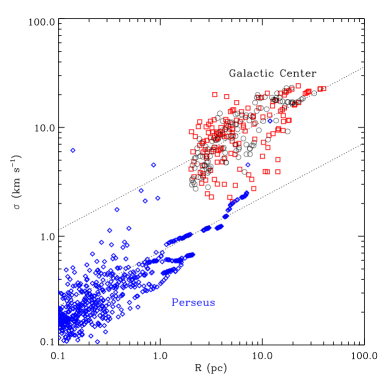
Figure 8: Comparison of the linewidth-size of structures traced by N₂H⁺ (black circles) and HCN (red squares) in the Galactic Centre with ¹³CO features from the Milky Way molecular cloud Perseus. Lower dashed line is the best fit relationship from Solomon et al. (1987), $\sigma=0.7R^{0.5}$. Upper dashed line is the same relationship, but where the coefficient is 3.6.

As a first comparison, and to validate our measurement approach, we compute the size-linewidth relationship from the dendrograms of ¹³CO observations of the Perseus molecular cloud. Optically thin ¹³CO emission traces both the diffuse molecular gas, as well as dense filaments and cores, within GMCs. It is therefore analogous to the dense gas tracers we consider for the CMZ, within which molecular gas is pervasive. Figure 8 shows the N₂H⁺ and HCN $\sigma-R$ relationship in the CMZ, along with the trend measured in Perseus. The ($\chi^{2}$) best fit line to the Perseus data is $\sigma=0.62R^{0.54}$. This relationship is similar to the best fit derived by Solomon et al. (1987), $\sigma=0.7R^{0.5}$, and is shown as the lower dashed line in Figure 8.

Clearly, the $\sigma$ – $R$ trend in the GC is similar to the local ISM, in that a comparable power-law index can account for the relationship across a range in spatial scale $R$ $\in 2-40$ pc. Yet, there is a systematic enhancement in dispersions, resulting in a coefficient that is about five times larger than the local ISM value (see Table 1). The upper dashed line in Figure 8 shows the local $\sigma$– $R$ relationship, enhanced by a factor of five. There is a reasonable agreement between this line and the linewidth-size trend measured in the GC, in agreement with the analysis by Oka et al. (1998, 2001) of individual and distinct CO clouds.

4.4 Interpreting the linewidth-size relationship

The agreement between the $\sigma$ – $R$ trend within a MC and between individual MCs has been interpreted as evidence for the “universality” of turbulence by Heyer & Brunt (2004). Namely, Heyer & Brunt (2004) suggest that turbulence observed in MCs originates on the largest scale in the ISM (see also Ossenkopf et al., 2001; Ossenkopf & Mac Low, 2002; Brunt et al., 2009). In their description, colliding flows in the diffuse ISM lead to the formation of MCs. While the MCs form at the interfaces of these colliding flows, they inherit the turbulent characteristics of the ambient ISM, leading to the observed “universal” $\sigma$ – $R$ relationship; smaller scale turbulence injection within MCs, e.g. due to internal supernovae or stellar winds, appear not to contribute substantially to the overall dispersions.

As we derive the linewidths in both the densest clouds and their surrounding medium, we can assess the relationship of the clouds and its environment. The relatively uniform linewidth-size trend in the CMZ, extending over an order of magnitude in spatial scales, may indeed reflect a scenario in which the dense clouds inherit the dynamic properties of the surrounding gas. Further, our analysis of the linewidths irrespective of the position within the PPV cubes (in Section 4.1) advocates for large scale driving as the primary source of turbulence. These results suggest that the transfer of turbulent energy across spatial scales in the CMZ occurs in a similar manner as in the more diffuse and quiescent ISM in the main disc of the Milky Way.

Nevertheless, the larger coefficient in the $\sigma-R$ relationship attests to some fundamental difference in the CMZ and the local ISM. The measured star formation rate in the CMZ is $\sim$50 times larger than the rate in the solar neighborhood (Yusef-Zadeh et al., 2009). Correspondingly, there is a higher rate of supernovae occurring in this starbursting environment. The variations in star formation activity are tied to the differences between the environmental properties of the main disk and CMZ. Namely, the total ISM density, vertical oscillation period (see e.g. Ostriker et al., 2010; Kim et al., 2011), and perhaps even shear levels set by the rotational velocity at a given Galactocentric radius, result in shorter dynamical times in the CMZ, and the associated cloud formation and destruction timescales. In the dense CMZ, the crowded sites of star formation and supernovae result in a higher frequency of colliding streams, relative to the main disc. These distributed supernovae may be a primary source of turbulence (Ostriker & Shetty, 2011; Shetty & Ostriker, 2012), which would be external to any given dense cloud. In the main disc, GMCs are relatively isolated from each other, so that supernovae are not distributed, resulting in a lower frequency of colliding shells. Coupled with the larger densities and temperatures, the ambient pressure in the CMZ is higher than the rest of the Milky Way. The enhanced turbulent velocity, and correspondingly the larger coefficient in the linewidth-size relationship, is likely associated to the higher degree of star formation activity in the CMZ.

The relationship between turbulent velocities, cloud sizes, masses, and the other physical properties of the ISM is germane for developing theoretical descriptions of the star formation process. Recent theoretical efforts have focused on the role of turbulence in regulating star formation (e.g. Krumholz et al., 2012; Ostriker et al., 2010; Ostriker & Shetty, 2011). Numerical simulations of self-regulating starbursting systems where distributed supernovae driven feedback balances the vertical weight of the disk produce turbulent velocities in dense gas of order 5 – 10 km s^-1 (Shetty & Ostriker, 2012), similar to the dispersion of the (presumably densest) clouds occurring on the smallest scales in Figure 2. In these models, the large scale dynamics drives the evolution of gas on smaller scales, including the velocity dispersion and ultimately star formation in dense gas. Quantifying the dynamical properties of the ISM will further constrain the numerical simulations and the affiliated description of star formation in similar starbursting environments.

As more observations resolve the structure and dynamics of a variety of environments, a direct comparison of characteristics of the local ISM will undoubtedly unfold. Dust and/or spectral line observations from lower density tracers will allow for estimates of the masses of the structures in the CMZ (e.g. Longmore et al., 2012). Combined with the $\sigma-R$ relationship, the full dynamic state of the clouds and ambient ISM should emerge. ALMA will be ideal for carrying out such an analysis, and reveal the similarities and differences between starbursting regions like the CMZ and the more quiescent environments, ultimately leading to a thorough understanding of the ISM.

5 Summary

We have measured the linewidths and sizes of structures in the observed N₂H⁺, HCN, H¹³CN, and HCO⁺ PPV cubes of the CMZ. Iso-intensity contours in the PPV cubes identify contiguous structures, from which we measure the linewidths and projected sizes. The ensemble of structures clearly portrays a linewidth $\sigma$ which increases with size $R$, with $\sigma$ $\sim$ 2 – 30 km s^-1 for structures with $R$ $\in$ 2 – 40 pc.

Employing a Bayesian regression analysis, we showed that the four tracers all produce similar linewidth-size power-law relationships. Fits from the tracers with the lowest noise levels, optically thin N₂H⁺ and optically thick HCN, produce indices $b\in 0.3-1.1$, and coefficients $A\in 0.9-4.7$ (Section 3).

By randomly shifting the iso-intensity contours within which $\sigma$ is measured, we demonstrated that the measured $\sigma-R$ trend is rather independent of the presence of dense structures. Therefore, turbulent velocities are predominantly driven on the largest scales in the CMZ, in agreement with interpretations of the ISM in the Milky Way disk. That there is no strong evidence for a flattening of the $\sigma-R$ relationship in the CMZ suggests that turbulence is driven on scales  $\buildrel>\over{\sim}$ 30 pc (Section 4.1). We also discussed that the morphology of structures and its velocities is (to some extent) likely to be determined by the nature of the underlying turbulent but coherent velocity field (Section 4.2).

We compared the $\sigma-R$ trend in the CMZ to that derived from Perseus. A power law linewidth-size relationship with index 0.5, which describes the local ISM well, reasonably captures the characteristics derived in the CMZ. This may be suggestive of the similarity in which star forming clouds inherit the turbulent properties of the ambient gas out of which they form. However, the relationship in the CMZ requires a factor of five enhancement in the coefficient relative to the local $\sigma-R$ power-law (Section 4.3). The starbursting nature of the CMZ, along with its higher densities, temperatures, and the associated pressure increase may be responsible for the larger magnitudes in turbulent velocities.

References

- Ballesteros-Paredes & Mac Low (2002) Ballesteros-Paredes J., Mac Low M.-M., 2002, ApJ, 570, 734
- Beaumont et al. (2012) Beaumont C., Goodman A., Alves J., Lombardi M., Roman-Zuniga C., Kauffmann J., Lada C., 2012, ArXiv e-prints 1204.2557
- Bergin & Tafalla (2007) Bergin E. A., Tafalla M., 2007, ARA&A, 45, 339
- Bolatto et al. (2008) Bolatto A. D., Leroy A. K., Rosolowsky E., Walter F., Blitz L., 2008, ApJ, 686, 948
- Brunt et al. (2009) Brunt C. M., Heyer M. H., Mac Low M.-M., 2009, A&A, 504, 883
- Caselli & Myers (1995) Caselli P., Myers P. C., 1995, ApJ, 446, 665
- Falgarone et al. (1992) Falgarone E., Puget J.-L., Perault M., 1992, A&A, 257, 715
- Fukui & Kawamura (2010) Fukui Y., Kawamura A., 2010, ARA&A, 48, 547
- Gammie et al. (2003) Gammie C. F., Lin Y.-T., Stone J. M., Ostriker E. C., 2003, ApJ, 592, 203
- Gelman et al. (2004) Gelman A., Carlin J. B., Stern H. S., Rubin D. B., 2004, Bayesian Data Analysis: Second Edition. Chapman & Hall
- Heyer et al. (2009) Heyer M., Krawczyk C., Duval J., Jackson J. M., 2009, ApJ, 699, 1092
- Heyer & Brunt (2004) Heyer M. H., Brunt C. M., 2004, ApJL, 615, L45
- Issa et al. (1990) Issa M., MacLaren I., Wolfendale A. W., 1990, ApJ, 352, 132
- Jones et al. (2012) Jones P. A. et al., 2012, MNRAS, 419, 2961
- Kalberla & Kerp (2009) Kalberla P. M. W., Kerp J., 2009, ARA&A, 47, 27
- Kauffmann et al. (2010a) Kauffmann J., Pillai T., Shetty R., Myers P. C., Goodman A. A., 2010a, ApJ, 712, 1137
- Kauffmann et al. (2010b) Kauffmann J., Pillai T., Shetty R., Myers P. C., Goodman A. A., 2010b, ApJ, 716, 433
- Kelly (2007) Kelly B. C., 2007, ApJ, 665, 1489
- Kim et al. (2011) Kim C.-G., Kim W.-T., Ostriker E. C., 2011, ApJ, 743, 25
- Krumholz et al. (2012) Krumholz M. R., Dekel A., McKee C. F., 2012, ApJ, 745, 69
- Krumholz & McKee (2005) Krumholz M. R., McKee C. F., 2005, ApJ, 630, 250
- Kruschke (2011) Kruschke J. K., 2011, Doing Bayesian Data Analysis. Elsevier Inc.
- Larson (1981) Larson R. B., 1981, MNRAS, 194, 809
- Leisawitz (1990) Leisawitz D., 1990, ApJ, 359, 319
- Longmore et al. (2012) Longmore S. N. et al., 2012, ApJ, 746, 117
- Mac Low & Klessen (2004) Mac Low M., Klessen R. S., 2004, Reviews of Modern Physics, 76, 125
- McKee & Ostriker (2007) McKee C. F., Ostriker E. C., 2007, ARA&A, 45, 565
- Miyazaki & Tsuboi (2000) Miyazaki A., Tsuboi M., 2000, ApJ, 536, 357
- Morris & Serabyn (1996) Morris M., Serabyn E., 1996, ARA&A, 34, 645
- Oka et al. (1998) Oka T., Hasegawa T., Hayashi M., Handa T., Sakamoto S., 1998, ApJ, 493, 730
- Oka et al. (2001) Oka T., Hasegawa T., Sato F., Tsuboi M., Miyazaki A., Sugimoto M., 2001, ApJ, 562, 348
- Ossenkopf et al. (2001) Ossenkopf V., Klessen R. S., Heitsch F., 2001, A&A, 379, 1005
- Ossenkopf & Mac Low (2002) Ossenkopf V., Mac Low M.-M., 2002, A&A, 390, 307
- Ostriker et al. (2010) Ostriker E. C., McKee C. F., Leroy A. K., 2010, ApJ, 721, 975
- Ostriker & Shetty (2011) Ostriker E. C., Shetty R., 2011, ApJ, 731, 41
- Padoan & Nordlund (2011) Padoan P., Nordlund Å., 2011, ApJ, 730, 40
- Pichardo et al. (2000) Pichardo B., Vázquez-Semadeni E., Gazol A., Passot T., Ballesteros-Paredes J., 2000, ApJ, 532, 353
- Purcell et al. (2006) Purcell C. R. et al., 2006, MNRAS, 367, 553
- Purcell et al. (2009) Purcell C. R., Longmore S. N., Burton M. G., Walsh A. J., Minier V., Cunningham M. R., Balasubramanyam R., 2009, MNRAS, 394, 323
- Ridge et al. (2006) Ridge N. A. et al., 2006, AJ, 131, 2921
- Rodriguez-Fernandez & Combes (2008) Rodriguez-Fernandez N. J., Combes F., 2008, A&A, 489, 115
- Rosolowsky et al. (2008) Rosolowsky E. W., Pineda J. E., Kauffmann J., Goodman A. A., 2008, ApJ, 679, 1338
- Sheth et al. (2008) Sheth K., Vogel S. N., Wilson C. D., Dame T. M., 2008, ApJ, 675, 330
- Shetty et al. (2010) Shetty R., Collins D. C., Kauffmann J., Goodman A. A., Rosolowsky E. W., Norman M. L., 2010, ApJ, 712, 1049
- Shetty et al. (2011) Shetty R., Glover S. C., Dullemond C. P., Ostriker E. C., Harris A. I., Klessen R. S., 2011, MNRAS, 415, 3253
- Shetty & Ostriker (2012) Shetty R., Ostriker E. C., 2012, ArXiv e-prints 1205.3174
- Solomon et al. (1987) Solomon P. M., Rivolo A. R., Barrett J., Yahil A., 1987, ApJ, 319, 730
- Teuben (1995) Teuben P., 1995, in ASP Conf. Ser. 77: Astronomical Data Analysis Software and Systems IV, Shaw R. A., Payne H. E., Hayes J. J. E., eds., pp. 398–+
- Young & Scoville (1991) Young J. S., Scoville N. Z., 1991, ARA&A, 29, 581
- Yusef-Zadeh et al. (2009) Yusef-Zadeh F. et al., 2009, ApJ, 702, 178