Study of internal wave breaking dependence on stratification

Abstract

Mixing effect in a stratified fluid is considered and examined. Euler equations for incompressible fluid stratified by a gravity field are applied to state a mathematical problem and describe the effect. It is found out that a system of Euler equations is not enough for a formulation of correct generalized problem. Some complementary relations are suggested and justified. A numerical method is developed and applied for study of processes of vortex destruction and mixing progress in a stratified fluid. The dependence of vortex destruction on a stratification scale is investigated numerically and it is shown that the effect increases with the stratification scale. It is observed that the effect of vortex destruction is absent when the fluid density is constant. Some simple mathematical explanation of the effect is suggested.

1 Introduction

The system of Euler equations for an incompressible fluid stratified by a gravity field is considered. It is known that internal gravity waves can propagate within fluids stratified by density in a gravity field. Internal wave breaking is one of interesting nonlinear effects, which is characterized by disintegration of waves with formation of typical spots with intensive small-scale convection inside them. The spots are often termed convective or turbulent ones because the convection inside them looks like turbulence. Static stability in the fluid becomes recovered with the course of time, but the density inside the spot remains different from the surrounding stratification. The phenomenon of internal wave breaking going with formation of a convective spot often is termed ”internal wave mixing”.

The effect of internal wave breaking is often observed in the ocean. The phenomenon is registered in the atmosphere [5] as well. Broken down internal waves reorganize stratification with time. Therefore, it is impossible to understand and explain stratification of the ocean or the atmosphere without taking into account the effect. Intensive intermixing of water by internal waves creates good nutrient medium for plankton in the ocean. Regions of the ocean, where wave breaking happens, are generally places of heightened biological productivity. It stimulates growing interest to them and to the physical effect, being cause of heightened biological productivity.

Many papers are dedicated to experimental study of the phenomenon [6, 7, 8, 9, 10]. In McEwan’s experimental papers, the phenomenon has been studied by means of thin laser measurements. Internal waves were excited in a laboratory tank with sizes of $25\,\text{cm}\times 50\,\text{cm}\times 25\text{cm}$ filled with a stratified fluid. Stratification is formed by dependence of water saltiness on height. The liquid density in the tank varied with height only by 4%. Therefore, it is possible to term this stratification as a weak one. The composite experimental equipment including two lasers has allowed to watch very small-scale density fluctuations originated owing to vortex destruction in the stratified fluid and to discover many details of the effect under study. Observation of small-scale structures had been based on dependence of refraction index of light on liquid density. McEwan has discovered and studied different stages of evolution of wave breaking and mixing [9], [10]: overturning, development of interliving microstructure, restoring of static stability. According to experiments [9], [10], the initial phase of evolution of a nonlinear wave finishes formation of tongues of more heavy liquid inside more light, and vice versa. Further, the effect of overturning develops, and tongues disintegrate into waves of much smaller scales. The static stability is restored in course of time, but the fluid stratification becomes changed.

Let us discuss reasons of formation of tongues. The velocity field within a local vortex is inhomogeneous, and top speeds are achieved at some distance from the vortex center. It leads to formation of the tongue of a heavy liquid, permeating into strata of a light liquid, and of the tongue of a light fluid, permeating into strata of a heavy liquid. Different fluid particles cover different path lengths for the same time, and difference of path lengths increases with time. If we neglect influence of gravity, such fluid movement within a vortex of an elliptic shape leads to distortion of isopycnic lines (lines of equal density) and to reeling of isopycnic lines onto an ellipse. The ellipse semiaxes are determined by distances from the vortex center up to particles having top speeds in the vortex. Some thin layer structure in which stratums of light and heavy fluids are alternating is an outcome of local rotating fluid movement. Imposed gravity field gives birth to wave processes, and it entails breaking down of the regular thin layer structure. So, we observe mixing of the fluid.

Due to the phenomenon mechanism, whatever weak the stratification would be, the density gradients will become arbitrary large with the course of time. Therefore, when we start mathematical modeling of the phenomenon, it is natural to presume a solution of nonlinear fluid equations may be nonsmooth and may contain discontinuities. It seems to be of interest to study nondifferentiable, generalized solutions of hydrodynamic equations of a stratified incompressible fluid placed into a gravity field.

Further, the fluid is supposed to be an ideal one. Estimates show that dissipative effects are important at late stages of evolution. Therefore, the nondissipative problem is of certain interest. To be sure, taking into account of dissipative terms should increase solution smoothness. The smoothing action of dissipation is explained by inhibition of waves with scales smaller than some minimally possible scale dependent on dissipative constants. At numerical modeling, the smoothing action of dissipation shows one’s worth only if the grid step is less than the minimally possible scale. Often it is not advantageous or impossible to increase resolution up to a minimally possible scale. It is one more argument for study of a nondissipative problem.

Processes of mixing in viscous two-layer $3D-$ fluids with unstable stratification were numerically explored in [11], [12] (see also the literature quoted there). Authors for raising productivity of computations have utilized parallelizing of calculations. The present paper essentially differs from [11], [12] because in mentioned papers the instability develops at the expense of unstable stratification (a heavy liquid has been initially placed above a light one). In the present paper, the stratification is continuous and stable; but in time the instability develops in itself, that is, under other mechanism than in [11], [12]. The instability is shaped by an initial vortex as it occur in occur in experiments of [9], [10]. Furthermore, the problem under consideration is a two-dimensional one, and dissipative processes are not taken into account, excepting (3.6). As against the mentioned papers, we are interested not only in simulation outcomes, but also in substantiation of mathematical statement of the problem and in admissible numerical methods. It is explained by nontrivial items in the problem. Researched questions are important for viscous liquid as well.

Monographies [13], [14], and papers [15], [16], [17], [18], [19], [20] are dedicated to mathematical research of linear equations for small-amplitude internal waves. As for nonlinear Euler equations for incompressible fluid, correctness of many problems is not proved yet [21]. Multimode approach [2], in a finite-mode model directly related to McEwan experiment demonstrates important role of nonlinear dispersion [3] We study nonlinear equations and show that a system of Euler equations is not enough for statement of a correct generalized problem in case of a stratified fluid. The effects of wave overturning and fluid mixing are simulated numerically.

The study of dependence of phenomenon of vortex destructions on a stratification scale is another purpose of the research. By means of numerical experiments, we shall demonstrate the decreasing of overturning effects with diminution of stratification scale $H$. On the contrary, the effect grows with increasing stratification scale $H$. Nevertheless, it have been discovered that if we take a limiting case when the fluid density is a constant, the effect of vortex destruction is absent.

2 Basic system of equations

We suppose a fluid behavior is described by Euler equations for an incompressible fluid

$$\frac{\partial\rho}{\partial t}+\frac{\partial\rho u}{\partial x}+\frac{\partial\rho w}{\partial z}=0,\qquad\frac{\partial\rho u}{\partial t}+\frac{\partial\rho u^{2}}{\partial x}+\frac{\partial\rho uw}{\partial z}=-\frac{\partial p}{\partial x},$$ (2.1)

$$\frac{\partial\rho w}{\partial t}+\frac{\partial\rho uw}{\partial x}+\frac{\partial\rho w^{2}}{\partial z}=-\frac{\partial p}{\partial z}-\rho g,\qquad\frac{\partial u}{\partial x}+\frac{\partial w}{\partial z}=0\text{.}$$

Here $\rho$ is the density, $p$ is the pressure, $u$ and $w$ are the horizontal and vertical mass velocities of the fluid, $t$ is time, $x,z$ are the horizontal and vertical coordinates respectively, $g$ is the free fall acceleration.

It is supposed as well that the nonperturbed fluid is stratified in density exponentially:

$$\rho_{0}(z)=\rho_{00}\exp\left(-\frac{z}{H}\right),\qquad H=6.23\,\text{m},\qquad\rho_{00}=1000\,\text{kg}/{\text{m}}^{3}.$$

The chosen value of $H$ approximately corresponds to the one for McEwan’s experiments [9], [10]. In considered McEwan’s experiments, the density stratification was linear, but the stratification scale was much greater than the size of the tank; therefore, the linear and exponential stratifications are practically indiscernible. An exponential stratification is more convenient for mathematical research of the equations.

The boundary condition is $\left(\textbf{v},\textbf{n}\right)=0$ at the boundary $\partial\Omega$ of the domain $\Omega$, where $\textbf{v}=\left(u,w\right)$ and n is a normal line to the boundary. Keeping in mind McEwan’s experiments, we take a rectangle with horizontal dimension $50\,\text{ cm}$ and vertical dimension $25\;\text{ cm}$ as the domain $\Omega$.

3 Statement of the generalized problem

3.1 Preliminary analysis

One of tested methods of numerical integration of Euler equations (2.1) was based on Galerkin method [22]. The solution was searched for as a series in terms of functions dependent on vertical coordinate $z$ and belonging to a complete orthogonal system of functions, the expansion coefficients were dependent on horizontal coordinate $x$ and time $t$. From Euler equations, by known recipe we have deduced the equations for expansion coefficients [3]. We term these equations as a set of equations for wave modes. The set of equations for wave modes have been solved numerically, and then the velocity and density have been calculated using the series.

In such a way we successfully simulated an initial phase of evolution of the nonlinear wave, which was finished with formation of tongue of a heavy liquid inside a light one, and vice-versa. A typical scale of the tongues is about $2\,\text{cm}$. Formation of such tongues is (observed) watched in laboratory experiments as well. In laboratory experiments, these tongues further disintegrate into waves of very small scales. However, we have miscarried this effect, though formally it is possible to obtain solution of the problem for all time.

In-depth study of the problem has given the discovery that it is impossible to simulate correctly the nonlinear process under study within the framework of a standard Galerkin method. The reason is that partial derivatives do not exist for functions with discontinuities. In such cases we should search for the nondifferentiable solution as a generalized, nonclassical one. In 1954, Lax, considering quasilinear equations, has shown that nonlinear equations admit definition of different, nonequivalent classes of generalized solutions [23], [24], [25], [26], (see also [27]).

It is explained by the fact the main equations are crashed at discontinuity surfaces, so we need some additional conditions to match solutions on discontinuity surfaces. However, the conditions surface may be taken different, if we consider the question only from a mathematical standpoint. Therefore, convergence and stability of the numerical method yet do not guarantee that an obtained generalized solution is valid from the physical point of view. Moreover, only one of possible definitions of a generalized solution may fit the physical sense. Sufficient conditions of physical validity of the generalized solution are not formulated yet, but necessary requirements are obvious. A generalized solution being adequate to the physical sense, should meet the condition of conservation of mass, momentum and energy.

The considered equations for incompressible fluid differ from surveyed by Lax (in what sense), but Lax’s argumentation is applicable to them as well. Analysis has shown that the conventional Galerkin method does not allow achieving simultaneous conservation of mass, momentum and energy for an obtained nondifferentiable solution. May be it is possible to correct somehow conventional Galerkin method that would allow to simulate correctly solutions with discontinuities. However, the authors cannot offer acceptable adjusting of a Galerkin method. At the same time, finite-difference methods give major freedom that permits choosing a numerical scheme ensuring warranted realization of fundamental conservation laws.

3.1.1 Energy functionals in the theory of linearized hydrodynamic equations for the stratified fluid

First, we remind how the theorems of existence, uniqueness and stability for linear problems are proved. Ordinarily linear wave equations possess some quadratic functional conserved over solutions. This conserved quadratic functional is called a wave energy functional. For example, if we linearize equations (2.1) with respect to a background density, we come to known equations of the theory of small-amplitude internal waves for which the law of wave energy conservation is (particular in [4, 28]):

$$\frac{dH_{lin}}{dt}=0,\qquad H_{lin}=\frac{1}{2}\int_{\Omega}\rho_{0}\left(z\right)\left[\left(\,u^{2}+w^{2}\right)+g\,H\,\phi^{2}\right]\,\,d\,\Omega$$ (3.1)

Here the function $\phi(x,z,t)$ is defined by the formula $\rho\left(x,z,t\right)=\rho_{0}\left(z\right)\left(1+\phi(x,z,t)\right)$. In (3.1) the term containing velocities means a kinetic energy, and the term containing $\frac{1}{2}g\,H\,\phi^{2}$ is a potential energy. Functional (3.1) is of great importance in mathematical theory of equations for small-amplitude waves: proofs of theorems of existence, uniqueness, stability for the linearized hydrodynamic equations essentially uses conservation of functional $H_{lin}$ over solutions.

The linearized fluid equations also possess other conservative functional of energy

$$E_{lin}=\int_{\Omega}\rho_{0}\left(z\right)\left[\frac{1}{2}\left(\,u^{2}+w^{2}\right)+g\,z\,\phi\right]\,\,d\,\Omega$$ (3.2)

We will name this functional a functional of hydrodynamic energy [29]. In (3.2), the term containing velocities means the kinetic energy and the term containing $g\,z\,\phi$ is the potential energy.

Here both conservative energy functionals are written to underline their distinction. Different formulas for energy functional are possible because energy is determined up to a constant. If we add any other conservative functional to the energy functional, we obtain a conservative functional again, which we may term an energy functional, but the expression for energy density becomes other. Therefore, different formulas for energy functional exist.

We have selected the form of wave energy functional (3.1) so that the energy to be zero at lack of waves. For this reason, functional (3.1) is named wave energy functional. Functional (3.2) is more known, but not possesses necessary mathematical properties.

3.1.2 Wave energy functional for nonlinear equations

Having the purpose to develop a theory for nonlinear equations, it is naturally to extend wave energy functional (3.1) to nonlinear case. The following theorem is valid.

Theorem 1.

Let a solution to equations (2.1) be differentiable. Then the functional

$$H_{nonl}=\int\limits_{\Omega}\left[\rho\,\frac{u^{2}+w^{2}}{2}+\rho\,g\,z+\,g\,H\,\left(\rho\,\ln\left(\frac{\rho}{\rho_{0}\left(0\right)}\right)+\,\left(\rho_{0}(z)-\rho\right)\right)\right]\,\,d\,\Omega\qquad$$ (3.3)

is conserved on solutions. The integrand in (3.3) is strictly non-negative at $\rho\geq 0$. The functional (3.3) turns into the functional (3.1), when we take the small-amplitude limit.

Proof.

Conservation of the functional (3.3) follows the fact that it is the sum of conservative functionals of the hydrodynamic energy $\int\limits_{\Omega}\left(\rho\,\frac{u^{2}+w^{2}}{2}+\rho\,g\,z\right)\,\,d\,\Omega$, of the mass $\int\limits_{\Omega}\rho\,\,d\,\Omega$, and of the conservative functionals $\int\limits_{\Omega}$ $\rho\,\ln\rho\,\,d\,\Omega$ and $\int\limits_{\Omega}q(z)\,\,d\,\Omega$. Nonnegativity of the term $\rho\,\frac{u^{2}+w^{2}}{2}$ is obvious at $\rho>0$. To prove nonnegativity of remaining summands of the integrand, we consider

$$a=\rho\,g\,z+\,g\,H\,\left(\rho\,\ln\left(\frac{\rho}{\rho_{0}\left(0\right)}\right)+\,\left(\rho_{0}(z)-\rho\right)\right)$$

We substitute $\rho=\rho_{0}(z)\,\left(1+\eta\right)$. To be sure, the requirement $\rho>0$ is equivalent to $\eta>-1$. For derivative with respect to variable $\eta$, it is valid:

$$\frac{\partial a}{\partial\eta}=H\,ln(1+\eta)\,\rho_{0}(z)\,g,\qquad\frac{\partial^{2}a}{\partial\eta^{2}}=H\,\frac{1}{(1+\eta)\,}\,\rho_{0}(z)\,g\;>0\qquad\text{ at }\eta>-1.$$

Unique minimum of the function $a(\eta)$ corresponds to $\eta=0$. It is enough to be convinced that in the limit of small-amplitude waves the functional under study turns into (3.1). ∎

We term the functional (3.3) as a generalized functional of wave energy because in a small-amplitude limit it turns into wave energy functional (3.1) for linearized equations. At lack of wave disturbances, the integrand in 3.3) is equal zero. The idea of functional (3.3) form, is taken from the Hamilton formalism explained in [4]. Nevertheless, nonnegativity of the integrand, also some other important mathematical properties of the functional are discovered anew.

Let us generalize (3.3) to a case when a solution may be nondifferentiable. The functionals of mass and hydrodynamic energy from which the functional is constructed (3.3), should be conserved for nondifferentiable solutions; it follows from their physical sense. However the functional
$\int\limits_{\Omega}\left[\,g\,H\,\left(\rho\,\ln\left(\frac{\rho}{\rho_{0}\left(0\right)}\right)\right)\right]\,\,d\,\Omega$ is not conserved in a case if the density field is nondifferentiable. Therefore, we demand that the following inequality have to be fulfilled

$$\frac{dH_{nonl}}{dt}\leq 0.$$ (3.4)

The sign ”$\leq$” is chosen because the sign ”$>$” in (3.4) leads to an unstable problem. We will use (3.3) and (3.4) as a basis of the theory of generalized solutions to nonlinear equations. Inapplicability of Hamilton formalism for considering of solutions with discontinuities of density follows from (3.3), (3.4).

3.1.3 Generalized solutions to the nonlinear problem

Preliminary analysis.

The equations (2.1) are written in a conservative form, in the form of fundamental conservation laws. From the physical point of view, the set of equations (2.1) is incomplete because it does not include the energy conservation law. Let $\omega\subset\Omega$ be an arbitrary star domain with piecewise smooth boundary, and let $S(\omega)$ be a boundary surface of the domain $\omega$, $d\textbf{S}=dS\,\textbf{n}$, where $dS$ is a surface element of $S(\omega)$, and n is an outer normal vector to $S(\omega)$. We write an integral relation for energy

$$\int\limits_{\omega}e(x,z,t)d\Omega-\int\limits_{\omega}e(x,z,0)d\Omega-\int\limits_{0}^{t}\oint\limits_{S\left(\omega\right)}e(x,z,t)\,\textbf{v}(x,z,t)\,d\textbf{S}\,dt=0,\quad e=\rho\left(\frac{u^{2}+w^{2}}{2}+gz\right)$$ (3.5)

If the solution of our problem is differentiable, then (3.5) follows from (2.1); but if the solution does not belong to a class of differentiable functions, then relation (3.5) does not follow (2.1). Therefore, permitting nondifferentiable solutions, we have to include (3.5) into the system of general equations as an individual equation.

Eqations (2.1), (3.5) are not enough for statement of a correct problem. For stability of the nonlinear problem, relation (3.4) should be fulfilled as well. As conservation of energy functional (3.5) is postulated, the inequality

$$\frac{\partial}{\partial t}\left(f\left(\rho\right)\right)+\nabla\left(f\left(\rho\right)\textbf{v}\right)=\nu\leq 0,\qquad f\left(\rho\right)=\rho\ln\left(\rho\right),$$ (3.6)

follows (3.4) and (3.5). Apparent requirement of compatibility of the relation (3.6) with the continuity equation (2.1) results in conclusion that $\nu$ may be nonzero only at the points where $\rho$ is nondifferentiable.

Further we shall use $f\left(\rho\right)=\rho\ln\left(\frac{\rho}{\rho_{0}(0)}\right)$, where $\rho_{0}(0)$ is the maximum value of the density (on the bottom),

use of the function $f$ of fixed sign is more convenient.

Definition of a generalized solution.

Using the set of equations (2.1), we routinely build some integral relations for definition of a generalized solution

$$\int\limits_{\Omega}\rho_{s}(x,z,0)\rho(x,z,0)\,d\Omega+\int\limits_{Q_{T}}\left(\rho\frac{\partial\rho_{s}}{\partial t}+\rho u\frac{\partial\rho_{s}}{\partial x}+\rho w\frac{\partial\rho_{s}}{\partial z}\right)\,dQ_{T}=0,$$ (3.7)

$$\int\limits_{\Omega}u(x,z,0)\rho(x,z,0)\,u_{s}(x,z,0)\,d\Omega+\int\limits_{\Omega}w(x,z,0)\rho(x,z,0)w_{s}(x,z,0)\,\,d\Omega+$$

$$\int\limits_{Q_{T}}\left[\rho u\,\frac{\partial u_{s}(x,z,t)}{\partial t}+\rho u^{2}\,\frac{\partial u_{s}(x,z,t)}{\partial x}+\rho uw\,\frac{\partial u_{s}(x,z,t)}{\partial z}\right]\,\,dQ_{T}$$

$$+\int\limits_{Q_{T}}\left[\rho w\frac{\partial w_{s}(x,z,t)}{\partial t}+\rho uw\frac{\partial w_{s}(x,z,t)}{\partial x}+\rho w^{2}\frac{\partial w_{s}(x,z,t)}{\partial z}+\rho gw_{s}(x,z,t)\right]dQ_{T}=0.$$

The relations should be fulfilled for any $\rho_{s}(x,z,t)\in C_{0}^{\infty}\left(\Omega\right)\times C^{\infty}[0,T]$, $u_{s}(x,z,t)=\frac{\partial\psi_{s}}{\partial z}$, $w_{s}(x,z,t)=-\frac{\partial\psi_{s}}{\partial x}$, $\psi_{s}(x,z,t)\in C_{0}^{\infty}\left(\Omega\right)\times C^{\infty}[0,T]$, $\rho_{s}(x,z,T)=\psi_{s}(x,z,T)=0$. In equations (3.7), $Q_{T}=\Omega\times\left[0,T\right]$. For the basic functions (velocity components and density), it is convenient to introduce the stream function, $u(x,z,t)=\frac{\partial\psi(x,z,t)}{\partial z}$, $w(x,z,t)=-\frac{\partial\psi(x,z,t)}{\partial x}$, where $\psi$ is a curve in $\mathring{W}_{2}^{1}(\Omega)$ parameterized with time $t$ [25], [30], [31].

However, the above integral relations are not sufficient for unambiguous definition of a generalized solution. To be sure, we should supply the equations (3.7) with the relation (3.5) and the equation (3.6) in an integral form:

$$\int\limits_{\omega}f\left(\rho\left(x,z,t\right)\right)\,d\Omega-\int\limits_{\omega}f\left(\rho\left(x,z,0\right)\right)\,d\Omega+\int\limits_{0}^{t}\oint\limits_{S(\omega)}f\left(\rho\left(x,z,t\right)\,\right)\textbf{v}\left(x,z,t\right)\,d\textbf{S}\,dt=\int\limits_{0}^{t}\int\limits_{\omega}\nu\left(x,z,t\right)d\Omega dt\leq 0.\qquad$$ (3.8)

Here $S(\omega)$ is a surface of star domain $\omega$ with smooth boundary. Below, we formulate working definition of the generalized solution.

We construct here a definition of a generalized solution, which should be acceptable from physical point of view and mathematically correct. From the previous reviewing, it is evident that (3.7) is not enough to find uniquely a physically justified generalized solution. It is necessary to supply (3.7) with requirements (3.5), (3.8), or with equivalent ones. If

$$\rho(x,z,t),\,\rho(x,z,t)u^{2}(x,z,t),\,\rho(x,z,t)w^{2}(x,z,t)\,\in L_{1}\left(Q_{T}\right),$$ (3.9)

$$\rho(x,z,0),\,\rho(x,z,0)u^{2}(x,z,0),\,\rho(x,z,0)w^{2}(x,z,0)\,\in L_{1}\left(\Omega\right),$$

then relations (3.7) have clear mathematical sense. Requirements (3.9) seem to be natural. Therefore, at analysis of (3.5), (3.8), we assume that requirements (3.9) are fulfilled. If the solution is piecewise-continuous and restricted in $Q_{T}$, then all integrals in (3.8), (3.5) exist; and it follows (3.8), that (3.5)

$$\int_{\Omega}e\left(x,z,t\right)\,d{\Omega}=\int_{\Omega}e\left(x,z,0\right)\,d{\Omega}.$$ (3.10)

$$\int\limits_{\Omega}f(x,z,t_{1})d\Omega\leq\int\limits_{\Omega}f(x,z,t_{2})d\Omega\qquad\text{for \; all}\quad t_{1}>t_{2},$$ (3.11)

A hypothetical case when requirements (3.9) are fulfilled but the solution belongs to a class of functions, for which the surface integral in (3.5) is not defined, deserves special examination. In this case, it is possible to try to interpret a surface integral in (3.5) as a pair of functionals ( $x$ and $z$ components). It is important that these functionals exist for any star-shaped domain $\omega$ with smooth boundary $S(\omega)$ and the functionals are additive ones. That is, if $\omega=\omega_{1}\cup\omega_{2}$, $\omega_{1}\cap\omega_{2}=\emptyset$, then a functional over surface $S(\omega)$ is equal to sum of functionals over surfaces $S(\omega_{1})$ and $S(\omega_{2})$, and relations (3.10) and (3.5) are fulfilled. One can easily be convinced that if requirements (3.9) and (3.10) are fulfilled, then such functionals can always be defined. Therefore, for definition of the generalized solution, we demand realization of (3.9), (3.10); at the same time, relation (3.5) is not utilized in explicit form. Analogous analysis reveals that condition (3.11) has to play an important role in definition of the generalized solution, but it is possible to not use (3.8) resulted in (3.11).

Definition 1.

Let $\textbf{v}(x,z,t)=\left(u(x,z,t),w(x,z,t)\right)$. We term $\lambda(x,z,t)=\left(\begin{array}[]{c}\rho(x,z,t)\\ \textbf{v}(x,z,t)\end{array}\right)$ as a generalized solution of equations (2.1), if $u(x,z,t)=\frac{\partial\psi(x,z,t)}{\partial z}$, $w(x,z,t)=-\frac{\partial\psi(x,z,t)}{\partial x}$, $\left.\psi\right|_{\partial\Omega}=0$ and if (3.7) (3.9), (3.10), (3.11), are fulfilled for any $\rho_{s}(x,z,t)\in C_{0}^{\infty}\left(\Omega\right)\times C^{\infty}[0,T]$, $u_{s}(x,z,t)=\frac{\partial\psi_{s}}{\partial z}$, $w_{s}(x,z,t)=-\frac{\partial\psi_{s}}{\partial x}$, $\psi_{s}(x,z,t)\in C_{0}^{\infty}\left(\Omega\right)\times C^{\infty}[0,T]$, $\rho_{s}(x,z,T)=\psi_{s}(x,z,T)=0$.

Remark 1.

For Navier-Stokes equations, the energy conservation law is not included into the system of constitutive equations, but the solution belongs the class $\mathring{V}_{2}\left(Q_{T}\right)$ [32]; and the energy relation follows Navier-Stokes equations for functions belonging to $\mathring{V}_{2}\left(Q_{T}\right)$ [32], [33]. In our case, an energy relation does not follow from integral relations (3.7), and the energy relation is imposed independently. Per se, we apply the condition of conservativeness (conservation of mass, energy) widely used in gas dynamics. In fact only the condition (3.11) important for inhomogeneous liquid, is novel. The condition (3.11) is important for viscous liquid as well. Fluid of constant density $\rho\equiv 1$ was studied in known monographs [32], [33].

4 Simulation of vortex destruction

We take the initial condition:

$$\rho\left(x,z,0\right)=\rho_{0}\left(z\right),\qquad\psi\left(x,z,0\right)=A\,\exp\left\{-\left[\left(\frac{x-x_{0}}{l_{x}}\right)^{2}+\left(\frac{z-z_{0}}{l_{z}}\right)^{2}\right]\right\},\qquad$$ (4.1)

where $l_{x}=0.16\;\text{m}$, $l_{z}=0.052\;\text{m}$, $A=-0.0095\;\text{m}^{2}/\text{s}$, $x_{0}=0.5\;\text{m}$, $z_{0}=0.125\;\text{m}$. This initial condition approximately corresponds to the disturbance created from an oscillating paddle in the tank in MackEwan’s experiments [9], [10]. The horizontal scale is approximately twice more than the vertical one. The amplitude of a vertical velocity is of $5\;\text{cm/s}$, the amplitude of a level velocity is of $16\;\text{cm/s}$. The top speed of internal wave propagation in the tank within a linear approximation is $c=10\;\text{cm/s}$. That is, the fluid velocity amplitude exceeds the limit of linear wave propagation speed.

The solution procedure was grounded on numerical integration of the system of Euler equations (2.1) by finite-difference method. The fluid density for $t=3\,\text{s}$, $7\,\text{s}$, $8\,\text{s}$ is shown in fig. 1, 2, 3.

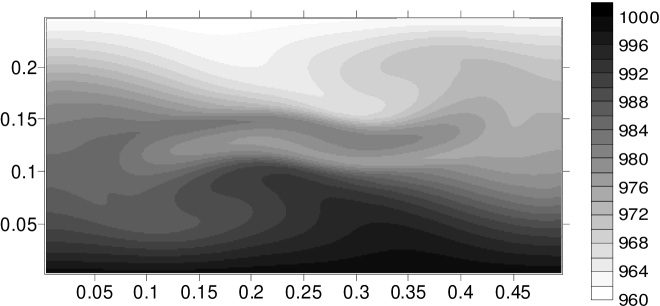
Figure 1: Fluid density at $t=3\,\text{s}$. $H=6.23\,\text{m}$, $h=0.25\,\text{cm}$.

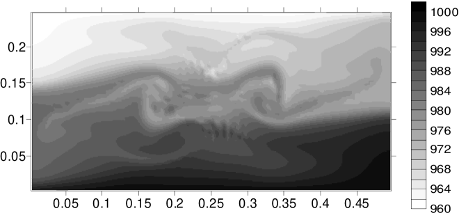
Figure 2: Fluid density at $t=7\,\text{s}$. $H=6.23\,\text{m}$, $h=0.25\,\text{cm}$.

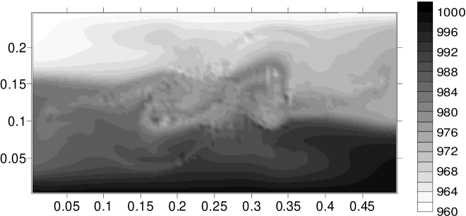
Figure 3: Fluid density at $t=8\,\text{s}$. $H=6.23\,\text{m}$, $h=0.25\,\text{cm}$

The overturning and formation of small-scale structures is advancing by formation of a tongue of a heavy liquid, penetrating into strata of a light liquid. Some layer structure containing segments with inverse density is generated as a result. At $t=5\,\text{s}$, abruptions arise in tongues, and isolated fragments of a light liquid arise inside a heavy liquid. At $t=7\,\text{s}$, the process of breaking becomes intensive. At $t=9\,\text{s}$, about $10\%$ of fluid in the tank is retracted in intensive small-scale convection. The vortex is atomized and the square of the convective spot slowly increases. However, with the course of time, small-sized blobs of a heavy liquid subside downwards, and blobs of a light fluid go upward. As a result, stable stratification is practically restored to the moment $t=14\,\text{s}$.

As a whole, the picture of wave breaking qualitatively coincides with the one circumscribed in [9], [10]. However, the last stage of reestablishing of continuous stratification is absent. It is explained by ignoring dissipative effects in the model.

The flow function is shown in figs. 4, 5.

Figure 4: Lines of the flow function at $t=3\,\text{s}$. $H=6.23\,\text{m}$, $h=0.25\,\text{cm}$

Figure 5: Lines of the flow function at $t=7\,\text{s}$. $H=6.23\,\text{m}$, $h=0.25\,\text{cm}$

At the first stage, the disturbance behavior is typical for internal waves and is perfectly explained by the theory of small-amplitude internal waves: left-hand and right-hand waves arise from this vortex. Because of the initial density perturbation is equal zero, the field of density perturbation is antisymmetric, and the field of a flow function is centrally symmetric. The symmetry is maintained in good approximation even when irregular movement is developed.

Irregular structures in the flow function appear later than in the density. Perhaps, it is explained by the fact that a flow function is an integral of velocity, hence it is the most smooth of considered physical fields. Two opposite jet flows are formed at $t=3\,\text{ s}$, and then they in unison create considerable velocity shift. The energy of small-scale waves is scooped from a considerable kinetic energy of the vortex due to instability development. It explains great intensity of the developed small-scale convection.

To verify exactness of our simulation, the outcomes of simulation with larger spatial step $h=0.5\,\text{cm }$ are shown for comparison in fig. 6, 7.

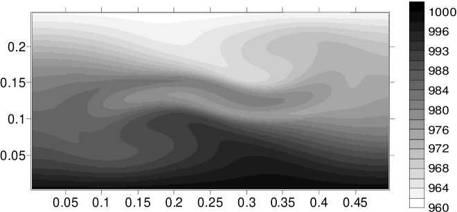
Figure 6: Fluid density at $t=3\,\text{s}$. $H=6.23\,\text{m}$, $h=0.5\,\text{cm}$

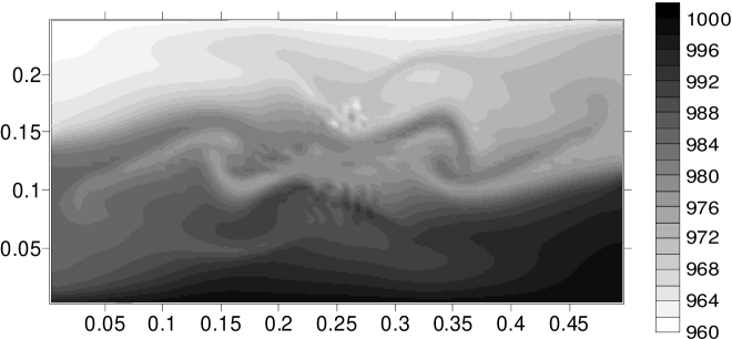
Figure 7: Fluid density at $t=7\,\text{s}$. $H=6.23\,\text{m}$, $h=0.5\,\text{cm}$

At $t\lessapprox 3\,\text{s}$, the simulation with the grid step $h=0.5\,\text{cm}$ coincide with the simulation with the scale $h=0.25\,\text{cm}$. At $t=5\,\text{ s}$, some small-scale structures arise, and simulations with different steps differ a little. The distinctions increase with time. However, rather high concurrence of the outcomes is kept. All large-scale details coincide.

4.1 Study of dependence of a vortex destruction on a stratification scale

Identical simulations of a vortex destruction for stratifications with doubled and twice diminished $H$ have been carried out for study of dependence of the phenomena on a stratification scale. Some outcomes for $H=3.1\,\text{m}$ are shown in fig. 8, 9. We see that when we decrease $H$, the evolution becomes an usual wave process. Fluid movement becomes more horizontal. The effect of wave breaking is starting later in spite of the fact that the inverse Brunt–Väisälä frequency is less. The wave breaking develops more slowly, and destruction runs languidly. Regular wave motion of the fluid is maintained as a whole, and only separate ”winged nuts”   are generated.

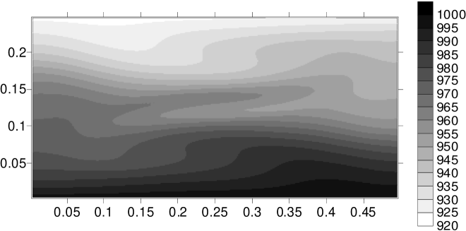
Figure 8: Fluid density in the tank at $t=3\,\text{s}$. $H=3.1\,\text{m}$, $h=0.25\,\text{cm}$

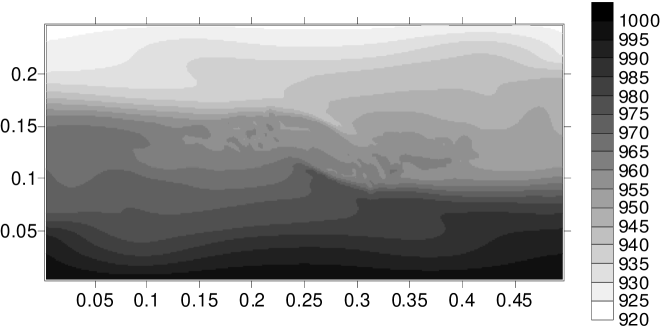
Figure 9: Fluid density in the tank at $t=7\,\text{s}$. $H=3.1\,\text{m}$, $h=0.25\,\text{cm}$

In fig. 10, 11, some outcomes of simulation of the same wave, but for stratification with doubled value of $H$, are shown. Comparison between the simulations relating to normal value of $H$ and the simulations relating to diminished twice $H$ displays that the phenomenon of vortex destruction and generation of small-scale convection is increased as $H$.

Figure 10: Field density in the tank at $t=3\,\text{s}$. $H=12.4\,\text{m}$, $h=0.25\,\text{cm}$

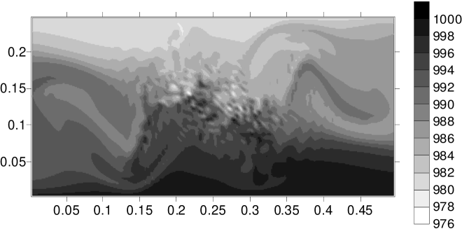
Figure 11: Fluid density in the tank at $t=7\,\text{s}$. $H=12.4\,\text{m}$, $h=0.25\,\text{cm}$

Therefore, we see that the vortex destruction effect grows with $H$, and a case of almost homogeneous fluid may be of interest. To consider the almost homogeneous fluid, we have carried out test simulation of evolution of the starting vortex for a stratification with very large $H=311,5\,\text{m}$. The considered fluid is almost homogeneous and the density is varied only by 0.08 %. The simulation outcomes are shown in Fig. 12, 13, 14. We see the wave collapses, and the time of starting of wave breakdown is the same as in case $H=12.4$ m. Therefore, for large $H$, the time of wave breakdown is determined not so much by value of $H$, as by starting conditions. If we consider the flow function, we discover the effect of formation of oppositely directed jet flows with velocity shear between them. Due to appearing this velocity shear, the instability arises. Small-scale fluctuations appear in the density field, and with some retardation, they appear in the flow function.

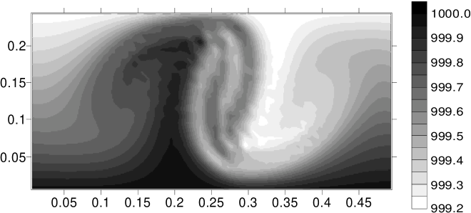
Figure 12: Fluid density in the tank at $t=3\;$ s. $H=311.5$ m. $h=0.25$ cm.

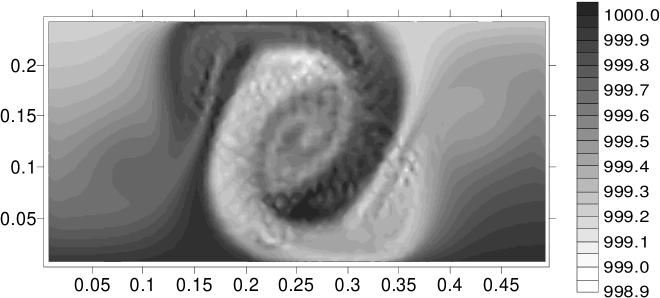
Figure 13: Fluid density in the tank at $t=6\;\text{s}$. $H=311.5$ m. $h=0.25$ cm.

Figure 14: The flow function lines at $t=7\;\text{s}$ in a stratication with $H=311.5$ m. $h=0.25$ cm.

Some late instant of evolution of the flow function for the same initial vortex, but in the fluid of a constant density, is shown in fig. 15. The fluid density is constant and is equal to the typical water density. We see that the vortex breakdown and formation of small-scale convection is absent in a strictly homogeneous medium, and only the vortex has become more symmetric. Perhaps, it is explained by the fact that any function $\psi(R)$, $R=\sqrt{(}x^{2}+z^{2})$ gives stationary solution to equations for homogeneous fluid. Therefore, the vortex takes a symmetric form in time.

Numerical simulations reveal that the phenomenon of breakdown becomes more and more brightly with increase of stratification scale $H$. Nevertheless, the phenomenon of vortex destruction is absent, when the fluid density is strictly a constant. It points out that continuous limit from a stratified fluid to the case of a fluid of constant density is absent for our initial conditions. The approximation of constant density is out of the physical sense in such cases, even if density variations are very small.

Figure 15: The flow function lines at $t=7\;\text{s}$ in a homogeneous fluid.

5 Explanation of the effect

Below we try to explain why evolution of a vortex in fluid of strict-constant density qualitatively differs from evolution of a vortex in fluid whose density is almost constant and varies within very narrow range.

Let us take $\rho\equiv 1$ for simplicity. Then the set of equations follows from (2.1)

$$\frac{\partial\xi}{\partial t}+u\,\frac{\partial\xi}{\partial x}+w\,\frac{\partial\xi}{\partial z}=0,$$ (5.1)

$$\frac{\partial^{2}\psi}{\partial x^{2}}+\frac{\partial^{2}\psi}{\partial z^{2}}=\xi.$$ (5.2)

In (5.1), $\xi=\frac{\partial u}{\partial z}-\frac{\partial w}{\partial x}$, $u(x,z,t)=\frac{\partial\psi}{\partial z}$, $w(x,z,t)=-\frac{\partial\psi}{\partial x}$. We assume that $\xi(x,z,0)$ is a continuous function, and $\max(|\xi(x,z,0)|)\leq M$. At the first step, we formally write a solution to (5.1) using a characteristic method and supposing the functions $u(x,z,t)$, $w(x,z,t)$ being known. The characteristic method gives us that $|\xi(x,z,t)|<sup(|\xi(x,z,0)|)$ and $\xi(x,z,t)\in L_{p}(\Omega)$ for any $p>0$. Applying the corollary of Sobolev embedding theorem [30], [31], we arrive at conclusion that the function $\psi(x,z,t)$ is continuous with respect to spatial variables, and $u(x,z,t)$, $w(x,z,t)$ are bounded ones. Moreover, the characteristic method also shows that all evolution of the starting vortex is only vortex deformation, but vortex destruction is impossible.

In case of weakly stratified fluid, the equation for $\xi$ is like this

$$\frac{\partial\xi}{\partial t}+u\frac{\partial\xi}{\partial x}+w\frac{\partial\xi}{\partial z}=Q,$$ (5.3)

$$\rho\,Q=g\frac{\partial\rho}{\partial x}-\frac{\partial\rho}{\partial z}\left[\frac{\partial u}{\partial t}+u\frac{\partial u}{\partial x}+w\frac{\partial u}{\partial z}\right]+\frac{\partial\rho}{\partial x}\left[\frac{\partial w}{\partial t}+u\frac{\partial w}{\partial x}+w\frac{\partial w}{\partial z}\right].$$

The equation for $\psi$ is the same, as (5.2). The right-hand terms containing square brackets are small against the first right-hand term in $Q$. Therefore, we ignore them and we consider only the approximation $\rho\,Q\approx g\frac{\partial\rho}{\partial x}$. We discussed at beginning of the paper that a starting vortex in a stratified fluid by all means shapes tongues of light and heavy fluids which become very thin in time. Therefore, very thin density structures arise in time. So, after some evolution, the term $|g\frac{\partial\rho}{\partial x}|$ becomes essential. This source $Q$ is of small scales and the one generates new vortices of smaller scales. These new small-scale vortices arise in weakly stratified fluid, and they should generate vortices of smaller scales in due time by means of the mechanism they arisen themselves. Therefore, we have a cascade process of generation of vortices of more and more small scales.

Example 1.

Any function $\psi\left(R\right)$, where $R=\sqrt{x^{2}+z^{2}}$ and $\psi\left(R\right)$ vanishes at infinity, satisfies (5.1,5.2). It gives a stationary solution. For example, we can take

$$\psi\left(R\right)=-\sqrt{\frac{g}{L}}\left(R+L\right)\exp\left(-\frac{R}{L}\right)\,,$$ (5.4)

where $L$ is a positive constant. We can easily do some analytical evaluations this such a function $\psi$. This current function describes rotation of the fluid with velocity $v\left(R\right)=\frac{d\psi}{dR}=\sqrt{\frac{g}{L}}\frac{R}{L}\exp\left(-R/L\right)$ dependent on the distance from the vortex center. This velocity field has maximum at $R=L$. We can consider (5.4) as approximate solution to (5.3), when we neglect of the term $\rho\,Q\approx g\frac{\partial\rho}{\partial x}$. Then we substitute (5.4) in continuity equation and calculate

$$\rho\left(x,z,t\right)=\rho_{0}\left(z-R*\sin\left(\frac{v(R)t}{2\pi R}\right)\right)=\rho_{0}\left(z-R*\sin\left(\sqrt{\frac{g}{L}}\frac{\exp\left(-R/L\right)t}{2\pi L}\right)\right).$$ (5.5)

At the following step, we calculate the source

$$\rho\,Q\approx g\frac{\partial\rho}{\partial x}=g\rho_{0}^{\prime}\left(z-R*\sin\left(\sqrt{\frac{g}{L}}\frac{\exp\left(-R/L\right)t}{2\pi L}\right)\right)*$$ (5.6)

$$\left[-\frac{x}{R}*\sin\left(\sqrt{\frac{g}{L}}\frac{\exp\left(-R/L\right)t}{2\pi L}\right)+\cos\left(\sqrt{\frac{g}{L}}\frac{exp\left(-R/L\right)t}{2\pi L}\right)*\left(\sqrt{\frac{g}{L}}\frac{\exp\left(-R/L\right)tx}{2\pi L}\right)\right]$$

Let stratification be linear and $\frac{d\rho_{o}}{dz}=-a$. We see that spacial derivatives of $\rho$ increase in time up to infinite values, and it is the reason we have used a technique of generalized solutions. For small $t$ we can neglect of the terms $u\frac{\partial\xi}{\partial x}+w\frac{\partial\xi}{\partial z}$ in ( 5.3) and integrate the equation ( 5.3):

$$\xi=\xi_{0}+\xi_{1}$$

$$\xi_{0}=-\sqrt{\frac{g}{L}}\left(2-\frac{R}{L}\right)\exp\left(-\frac{R}{L}\right)$$

$$\xi_{1}=-\frac{agx}{RL}\left\{2\pi\left(R+L\right)\left[\cos\left(\frac{\exp\left(-\frac{R}{L}\right)t}{2\pi}\right)-1\right]\exp\left(\frac{R}{L}\right)+Rt\sin\left(\frac{\exp\left(-\frac{R}{L}\right)t}{2\pi}\right)\right\}$$ (5.7)

Here $\xi_{0}$ corresponds to (5.4), and $\xi_{1}$ describes generation of new vortices. The expression for $\xi_{1}$ contains growing term $-\frac{agxt}{L}\sin\left(\frac{\exp\left(-\frac{R}{L}\right)t}{2\pi}\right)$, and due to presence of $\sin\left(\frac{\exp\left(-\frac{R}{L}\right)t}{2\pi}\right)$ this term starting some t is a function changing sign as a function of coordinates. It displays generation of new vortices in time owing to stratification influence.

We also note that other right-hand terms in $Q$ in (5.3) take into account inertial forces arising in flow moving with acceleration. This inertia forces are equivalent to presence of some gravity field. That is, the effect of cascade vortex destruction in a nonuniform fluid can start without gravity field, but when we apply accelerated movement to vortex motion.

6 Basic outcomes and conclusion

The system of Euler equations for an incompressible stratified fluid was studied. A non-negative nonincreasing functional extending wave energy functional of the theory of linearized Euler equations is suggested. The functional value is conserved over differentiable solutions, and diminishes if density discontinuities are present. Functional properties have allowed using it for analysis of statement of a generalized problem. It is shown that Euler equations are not enough for statement of a correct generalized problem in case of a stratified fluid in the gravity field. Some auxiliary conditions are formulated and justified. One of them is an energy conservation law, and the second is a special requirement for density (3.6). The statement of a generalized problem is formulated. The finite-difference problem-solving procedure is developed. Existence of a weak solution is proved.

The phenomenon of destruction of starting vortex in conditions of McEwan’s laboratory experiments [9], [10] has been simulated and studied. Qualitative concurrence of the simulated effect with the one observed in laboratory experiments, is good, but the last stage of restoring of smooth stratification is absent due to usage of an ideal liquid model. Some new data about the phenomenon, difficult for laboratory measurement, are obtained, and evolution of the flow function is studied. It is shown that large gradients appear in the velocity field at the expense of nonlinear effects and they may play an important role in development of instability.

By means of numerical experiments, dependence of the solution on a stratification scale $H$ is studied. It is revealed that the effects of vortex destruction and formation of small-scale convection grows with $H$ for strongly nonlinear waves. On the contrary, when we decrease $H$, the effect of wave destruction becomes weak. The wave breakdown is starting from the density field and some later formation of small-scale structures in the flow function is observed. The effect of vortex destruction is not observed when the fluid density is strictly a constant.

References

- [1] Kshevetskii S.P. Analytical and numerical investigation of nonlinear internal gravity waves. Nonlinear Processes in Geophysics. 2001. v.8. 37–53.
- [2] S. Leble Nonlinear Waves in Waveguides with stratification (Springer-Verlag, 1991),164p.
- [3] A. Halim, S. Kshevetskii, S. Leble Approximate solution for Euler equations of stratified water via numerical solution of coupled KdV system. IJMMS v 2003 N63, pp 3979-3993.
- [4] Miropolskii Yu.Z. Dynamics of internal gravity waves in the ocean. Leningrad. Gidrometeoizdat. 1981.
- [5] Pfister L., Starr W., Craig R., Lewenstein M., Legg M. Small-scale motions observed by aircraft in the tropical lower stratosphere: evidence for mixing and its relationship to large-scale flows. Journal of Atmospheric Sciences. 1986. v.43. 3210–3225.
- [6] Silva I.P.D.De, Imberger J., Ivey G.N. Localized mixing due to a breaking internal wave ray at a sloping bed. J. Fluid Mech. 1997. v.350. 1–27.
- [7] Silva I.P.D.De, Fernando H.J.S. Experement on collapsing turbulent regions in stratified fluid. J. Fluid Mech. 1998. v.358. 29–60.
- [8] Mason D.M., Kerswell R. Nonlinear evolution of the elliptical instability: an example of internal wave breakdown. J. Fluid Mech. 1999. v.396. P.73–108.
- [9] McEwan A.D. Degeneration of resonantly-excited standing internal gravity waves. J. Fluid Mech. 1971. v.50. 431– 448.
- [10] McEwan A.D. The kinematics of stratified mixing through internal wavebreaking. J.Fluid Mech. 1983. v.128. 47–57.
- [11] Zhmaylo V.A., Sin’kova O.G., Sofronov V.N., Statsenko V.P., Yanikin Yu. V., Guzhova A.R., Pavlunin A.S. Numerical study of gravitational turbulent mixing in alternating-sign acceleration. Parallel Computational Fluid Dynamics. Advanced numerical methods and applications. Elsevier. 2004. 235–241.
- [12] Tishkin V.F., Zmitrenko N.V., Ladonkina M.Ye., Proncheva N.G., Garina S.M. A study of a gravity-gradient mixing properties by means of direct numerical modelling. Advanced numerical methods and applications. Elsevier. 2004. 197–204.
- [13] Gabov S.A., Sveshnikov A.G. Linear problems of the theory of non-stationary internal waves. Moscow. Science. 1990.
- [14] Gabov S.A., Sveshnikov A.G. Problems of dynamics of stratified fluids. Moscow. Science. 1986.
- [15] Garipov R.M. On linear theory of gravity waves: theorem of existence and uniqueness. Arch. Rat. Mech. Anal. 1967. v.24, 352–362.
- [16] Gabov S.A., Sveshnikov R.A. About some problems linked with oscillations of stratified fluids. Differential equations. 1982. v.18, 1150–1156.
- [17] Gabov S.A., Malysheva G.J., Sveshnikov A.G., Shatov A.K. About some equations originating from dynamics of rotated, stratified and compressible fluid. Computational Mathematics and Mathematical Physics. 1984. v 24, 1850–1863.
- [18] Kopachevskij N.D., Temnov A.N. Free oscillation of ideal stratified fluid in a vessel. Computational Mathematics and Mathematical Physics. 1984. v.24, 109–123.
- [19] Kopachevskij N.D., Temnov A.N. Oscillation of stratified fluid in basin of arbitrary shape. Computational Mathematics and Mathematical Physics. 1986. v. 26, 734–755.
- [20] Gabov S.R. To the theory of internal waves at presence of free surface. Computational Mathematics and Mathematical Physics. 1988. v.28, 335–345.
- [21] Zeytounian R.Kh. Correctness of problems of dynamics of fluids (hydrodynamic point of view). Successes of Mathematical Sciences. 1999. v.54. 3–92.
- [22] Fletcher C.A.J. Computational Galerkin methods. Springer-Verlag. 1984.
- [23] Lax P.D. Weak solutions of nonlinear hyperbolic equations and their numerical computation. Comm. of Pure and Appl. Math. 1954, 159–193.
- [24] Lax P.D. Hyperbolic systems of conservation laws. II. Comm. Pure Appl. Math. 1957. v.10. 537–566.
- [25] Richtmayer R.D., Principles of advanced mathematical physics, V.1. Springer-Verlag, 1978.
- [26] Richtmayer R.D., Morton K.W. Difference Methods for initial-value problems. Interscience publishers. 1967.
- [27] Neumann J., Richtmyer R. A method for numerical calculation of hydrodynamic shocks. Journal of Applied Physics. 1950. V.21 232–237.
- [28] Monin A. Fundamental theory of geophysical hydrodynamics. Leningrad. Gidrometeoizdat. 1988.
- [29] Landau L.D., Lifshits E.M. Theoretical physics. v. 6. Hydrodynamics. Moscow. Science. 1988.
- [30] Sobolev S.L. Some applications of the functional analysis to mathematical physics. Moscow. Science. 1988.
- [31] Ladyzenskaya O.A. Boundary value problems of mathematical physics. M.: Science. 1973.
- [32] Ladyzenskaya O.A. Mathematical problems of dynamics of viscous incompressible fluid. Moscow. Science. 1970.
- [33] Temam R. Navier-Stokes equations. The theory and a numerical analysis. Moscow. World. 1981.
- [34] Kshevetskii S.P. Study of vortex breakdown in a sratified fluid. Computational mathematics and mathematical physics. 2006, v. 46, 11, pp. 2081-2098.