Time and frequency transfer with a microwave link in the ACES/PHARAO mission

Abstract

The Atomic Clocks Ensemble in Space (ACES/PHARAO mission), which will be installed on board the International Space Station (ISS), uses a dedicated two-way Micro-Wave Link (MWL) in order to compare the timescale generated on board with those provided by many ground stations disseminated on the Earth. Phase accuracy and stability of this long range link will have a key role in the success of the ACES/PHARAO experiment. SYRTE laboratory is heavily involved in the design and development of the data processing software : from theoretical modelling and numerical simulations to the development of a software prototype. Our team is working on a wide range of problems that need to be solved in order to achieve high accuracy in (almost) real time. In this article we present some key aspects of the measurement, as well as current status of the software’s development.

I Introduction

The ACES/PHARAO mission is an international metrological space mission aiming at realizing a time scale of high stability and accuracy on board the International Space Station (ISS). Relative frequency stability (ADEV) should be better than $\sigma_{y}=10^{-13}\cdot\tau^{-1/2}$, which corresponds to $3\cdot 10^{-16}$ after one day of integration (see fig.1); time deviation (TDEV) should be better than $2.1\cdot 10^{-14}\cdot\tau^{1/2}$, which corresponds to 12 ps after one day of integration (see fig.2). Absolute frequency accuracy should be around $10^{-16}$.

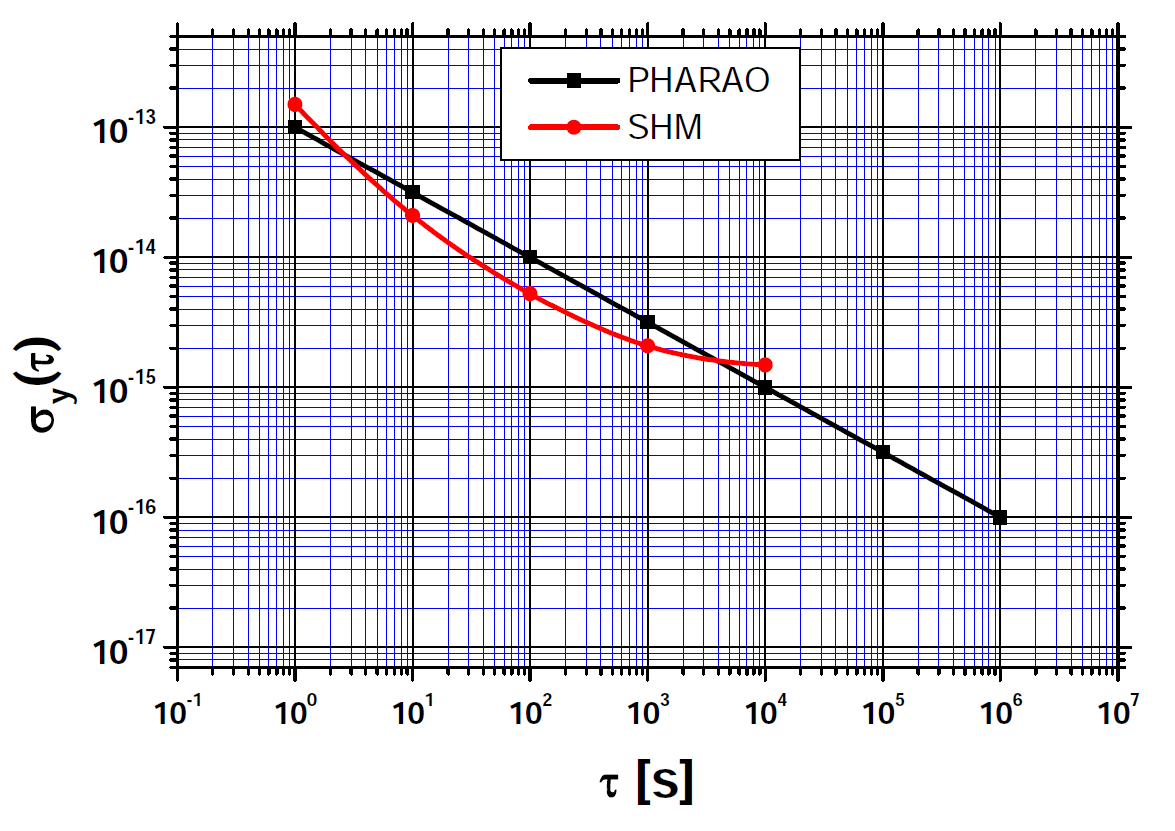
Figure 1: PHARAO (Cesium clock) and SHM (hydrogen maser) expected performances in Allan deviation.

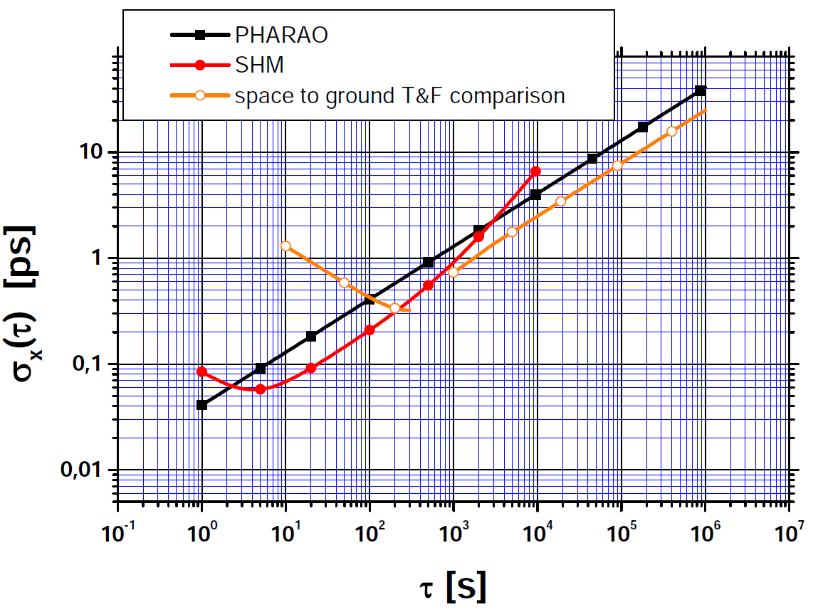
Figure 2: Performance objective of the ACES clocks and the ACES space-ground time and frequency transfer expressed in time deviation.

This mission is an international cooperation of more than 150 people. PI laboratories are SYRTE/Paris Observatory, LKB/ENS and Neuchâtel Observatory, and leading space agencies are the European Space Agency and CNES, the French space agency. Many industries are involved, the main ones being EADS/Astrium, TimeTech and Thales. All are working together to meet the scientific objectives of the mission:

• Demonstrate the high permformance of the atomic clocks ensemble in the space environment and the ability to achieve high stability on space-ground time and frequency transfer.

• Compare ground clocks at high resolution on a world-wide basis using a link in the microwave domain. In common view mode, the link stability should reach around 0.3 ps after 300 s of integration; in non-common view mode, it should reach a stability of around 7 ps after 1 day of integration (see fig.2).

• Perform equivalence principle tests. It will be possible to test Local Lorentz Invariance and Local Position Invariance to unprecedent accuracy by doing three types of tests: a test of gravitational red-shift, drift of the fine structure constant and of anisotropy of light.

Besides these primary objectives, several secondary objectives can be found in [1]. For example, if the theory of general relativity is considered as exact, then the measurement of gravitational redshifts can be used to measure gravitational potential differences between different clock locations. It is a new type of geodetic measurements using clocks called relativistic geodesy.

In this article we describe in details the Micro-Wave Link (MWL) used in the ACES/PHARAO mission, and developed by TimeTech (TT). First we describe one-way and two-way links theoretically and introduce the SYRTE Team (ST) observables. In the second part we describe how works the TT modem, and what is the link between the modem observables (TT observables) and the ST observables. Finally we present the status of the data analysis software and of the simulation we are developing.

II The Micro-Wave Link (MWL)

The Micro-Wave Link (MWL) will be used for space-ground time and frequency transfer. A time transfer is the ability to synchronize distant clocks, i.e. determine the difference of their displayed time for a given coordinate time. The choice of time coordinate defines the notion of simultaneity, which is only conventional. A frequency transfer is the ability to syntonize distant clocks, i.e. determine the difference of clock frequencies for a given coordinate time. Here we suppose that all clocks are perfect, i.e. their displayed time is exactly their proper time. Proper time $\tau$ is given in a metric theory of gravity by relation:

$$c^{2}{\text{d}}\tau^{2}=-g_{\alpha\beta}{\text{d}}x^{\alpha}{\text{d}}x^{\beta},$$ (1)

where $g_{\alpha\beta}$ is the metric, $c$ the velocity of light, $\{x^{\alpha}\}$ the coordinates and Einstein summation rule is used. We use in this article the notation $[.]$, which is the coordinate / proper time transformation obtained from eq.(1), and $T_{ij}=t_{j}-t_{i}$ for coordinate time intervals.

The MWL is composed of three signals of different frequencies: one uplink at frequency $\simeq 13.5$ GHz, and two downlinks at $\simeq 14.7$ GHz and 2.2 GHz. Measurements are done on the carrier itself and on a code which modulates the carrier. The link is asynchronous: a configuration can be chosen by interpolating observables. In the following we give a formal description of one-way and two-way links for code observables. The principle for carrier observables is the same except that periods cannot be identified, leading to a phase ambiguity.

II-A One-way link

II-A1 Experiment

(a) Sequence of events

(b) Space-time diagram

Figure 3: Schematic representation of the one-way link.

let’s consider a one-way link between a ground and a space clock represented respectively by subscript $g$ and $s$. The sequence of events is illustrated on fig.3. At time coordinate $t_{1}$, clock $g$ displays time $\tau_{1}$ and modem Mg produces a code $C^{1}$. This code modulates a sinusoidal signal of frequency $f$ and sent at coordinate time $t_{2}$ by antenna $g$. The delay between the code production and its transmission by antenna $g$ is $\Delta^{g}=[T_{12}]^{g}$, expressed in local frame of clock $g$. Antenna $s$ receives signal $C^{1}$ at coordinate time $t_{3}$, and transmit it to modem Ms and clock $s$ which receives it at coordinate time $t_{4}$, with a delay $\Delta^{s}=[T_{34}]^{s}$. Clock $s$ displays time $\tau_{1}$ and modem Ms produces the code $C^{1}$ at coordinate time $t_{5}$.

We use superscript $g$ or $s$ on proper times $\tau$ for clocks $g$ or $s$, and we express proper time as a function of coordinate time. Then we can write

$$\tau_{1}=\tau^{g}(t_{1})=\tau^{s}(t_{5}).$$ (2)

We define the ST (SYRTE Team) observable $\Delta\tau^{s}$ given by modem Ms with:

$$\Delta\tau^{s}(\tau^{s}(t_{4}))=\tau^{s}(t_{5})-\tau^{s}(t_{4}).$$ (3)

This observable is dated with proper time of clock $s$ when this clock receives code $C^{1}$ from antenna $s$. It can be interpreted as the difference between the time of production of code $C^{1}$ by clock $s$, and time of reception of same code $C^{1}$ sent by clock $g$, all expressed in proper time of clock $s$.

II-A2 Desynchronisation

desynchronisation between clock $g$ and $s$ is written in an hypersurface characterized by coordinate time $t=\text{constant}$. From eqs.(2)-(3) it is straightforward to deduce it for coordinate time $t_{4}$:

$$\tau^{s}(t_{4})-\tau^{g}(t_{4})=-\Delta\tau^{s}\left(\tau^{s}(t_{4})\right)-\left[T_{23}+\left[\Delta^{g}+\Delta^{s}\right]^{t}\right]^{g}$$ (4)

Similar formulas can be obtained for the desynchronization at coordinate times $t_{1}$ and $t_{5}$. This expression has been obtained for the uplink, from ground to space. To obtain the desynchronisation with downlink observables, all you have to do is replace $g$ and $s$ in eq.(4).

II-B Two-way link

II-B1 Experiment

let’s consider now a link which is composed of two one-way links, between a ground and a space clock represented respectively by subscript $g$ and $s$. The two sequences of events are illustrated on fig. 4. The uplink (from ground to space) has a frequency $f_{1}$ and is represented by coordinate time sequence $(t_{1}^{0},t_{1},t_{2},t_{2}^{0},t_{7}^{0})$ (fig.4(a)). This link is defined with the relation:

$$\tau^{g}(t_{1}^{0})=\tau^{s}(t_{7}^{0}).$$

The downlink has a frequency $f_{2}$ and is represented by coordinate time sequence $(t_{3}^{0},t_{3},t_{4},t_{4}^{0},t_{8}^{0})$ (fig.3(b)). This link is defined with the relation:

$$\tau^{s}(t_{3}^{0})=\tau^{g}(t_{8}^{0}).$$

(a) Uplink sequence of events

(b) Downlink sequence of events

(c) Space-time diagram

Figure 4: Schematic representation of the two-way link.

II-B2 Desynchronisation in a two-way configuration

a two-way configuration is defined by $\tau^{g}(t_{1}^{0})=\tau^{s}(t_{3}^{0})$, i.e. the code $C^{1}$ of link $f_{1}$ is the same as code $C^{2}$ of link $f_{2}$, and they are locally produced and sent at the same time: $t_{1}^{0}=t_{8}^{0}$ (at clock $g$) and $t_{3}^{0}=t_{7}^{0}$ (at clock $s$). Then we calculate desynchronisation between clocks $g$ and $s$ at coordinate time $t^{0}_{1}$ as:

$$\tau^{s}(t_{1}^{0})-\tau^{g}(t_{1}^{0})=\frac{1}{2}\left[\left[\Delta\tau_{\text{mo}}^{g}(t_{4}^{0})-\Delta\tau_{\text{mo}}^{s}(t_{2}^{0})\right]^{t}+T_{34}-T_{12}\right]^{s}$$ (5)

where we introduced the corrected observables $\Delta\tau_{\text{mo}}^{g}$ and $\Delta\tau_{\text{mo}}^{s}$:

$$\begin{array}[]{lcl}\Delta\tau_{\text{mo}}^{g}(t_{4}^{0})&=&\Delta\tau^{g}\left(\tau^{g}(t_{4}^{0})\right)+\Delta^{g}_{2}+\Delta^{s}_{2}\\[7.22743pt] \Delta\tau_{\text{mo}}^{s}(t_{2}^{0})&=&\Delta\tau^{s}\left(\tau^{s}(t_{2}^{0})\right)+\Delta^{g}_{1}+\Delta^{s}_{1}.\end{array}$$ (6)

II-B3 Desynchronisation in a $\Lambda$ configuration

in the ACES/PHARAO mission we use the so-called $\Lambda$ configuration. This configuration minimizes the error coming from the uncertainty on ISS orbitography (in [2] it has been shown that in this configuration the requirement on ISS orbitography is around 10 m). The $\Lambda$ configuration is defined by $t_{2}=t_{3}$, i.e. code $C^{2}$ is sent at antenna $s$ when code $C^{1}$ is received at this antenna. This configuration is obtained by interpolating the observables. Then it can be shown that desynchronisation between clocks $g$ and $s$ at coordinate time $t_{2}$ is:

$$\tau^{s}(t_{2})-\tau^{g}(t_{2})=\frac{1}{2}\left(\Delta\tau_{\text{mo}}^{g}(t_{4}^{0})-\Delta\tau_{\text{mo}}^{s}(t_{2}^{0})+\left[T_{34}-T_{12}\right]^{g}\right).$$ (7)

II-C Approximations

II-C1 Coordinate / proper time transformation

in equation (7) remains one transformation from coordinate to proper time. We know that $T_{12}\sim T_{34}\sim 1$ ms. During this time interval we can consider that the gravitational potential and velocity of the ground station are constant. Therefore we can do the approximation:

$$\left[T_{34}-T_{12}\right]^{g}=(1-\epsilon_{g}(t_{2}))\left(T_{34}-T_{12}\right),$$ (8)

where

$$\epsilon_{g}(t)=\dfrac{GM}{r_{g}(t)c^{2}}+\dfrac{v_{g}^{2}(t)}{2c^{2}},$$

$M$ is the Earth mass, $r_{g}(t)$ and $v_{g}(t)$ are the radial coordinate and the coordinate velocity of the ground clock at coordinate time $t$. Orders of magnitude of these corrective terms are:

$$\dfrac{GM}{r_{g}c^{2}}T_{34} \sim 0.6\ \text{ps}$$

$$\dfrac{v_{g}^{2}}{2c^{2}}T_{34} \sim 0.002\ \text{ps}$$

The gravitational term is just at the limit of the required accuracy. The velocity term is well below, so we can neglect it. Final formula for desynchronisation is then:

$$\tau^{s}(t_{2})-\tau^{g}(t_{2})=\frac{1}{2}\left(\Delta\tau_{\text{mo}}^{g}(t_{4}^{0})-\Delta\tau_{\text{mo}}^{s}(t_{2}^{0})\right.$$

$$+\left.\left(1-\frac{GM}{r_{g}(t_{2})c^{2}}\right)\left(T_{34}-T_{12}\right)\right).$$ (9)

II-C2 $\Lambda$ configuration

in the $\Lambda$ configuration we suppose that $T_{23}=0$. However, this will never be exactly 0 and it will be known with a precision $\delta T_{23}$. This will add a supplementary delay $\delta(\tau^{s}-\tau^{g})$ to desynchronisation (7):

$$\delta(\tau^{s}-\tau^{g})(t_{2})=\left(\epsilon_{g}(t_{2})-\epsilon_{s}(t_{2})\right)\delta T_{23}$$

Orders of magnitude are:

$$\dfrac{GM}{c^{2}}\left(\dfrac{1}{r_{g}}-\dfrac{1}{r_{s}}\right) \sim 2.8\ \cdot 10^{-11}$$

$$\dfrac{v_{g}^{2}-v_{s}^{2}}{2c^{2}} \sim -3.3\cdot 10^{-10}$$

With the required accuracy on the MWL, $|\delta(\tau^{s}-\tau^{g})|\lesssim 0.3$ ps, we deduce the following constraint on $\delta T_{23}$:

$$\delta T_{23}\lesssim 0.9\ \text{ms}.$$

This constraint is much less constraining than the one coming from orbitography, which is $\delta T_{23}\lesssim 1~{}\mu\text{s}$ (see [2]).

II-D Atmospheric delays

The downlink is composed of two one-way links of frequencies $f_{2}$ and $f_{3}$, represented respectively by coordinate time sequence $(t_{3}^{0},t_{3},t_{4},t_{4}^{0},t_{8}^{0})$ and $(t_{5}^{0},t_{5},t_{6},t_{6}^{0},t_{9}^{0})$. These two links are affected by a ionospheric delay that depends on their respective frequencies, whereas the tropospheric delay does not depend on the link frequency (we neglect dispersive effects). We write:

$$T_{34} =\frac{R_{34}}{c}+\Delta^{\text{iono}}_{34}(f_{2})+\Delta^{\text{tropo}}_{34}$$

$$+\dfrac{2GM}{c^{3}}\ln\left(\dfrac{r_{\text{Tx}}(t_{3})+r_{\text{Rx}}(t_{4})+R_{34}}{r_{\text{Tx}}(t_{3})+r_{\text{Rx}}(t_{4})-R_{34}}\right)+\mathcal{O}(c^{-4})$$ (10)

$$T_{56} =\frac{R_{56}}{c}+\Delta^{\text{iono}}_{56}(f_{3})+\Delta^{\text{tropo}}_{56}$$

$$+\dfrac{2GM}{c^{3}}\ln\left(\dfrac{r_{\text{Tx}}(t_{5})+r_{\text{Rx}}(t_{6})+R_{56}}{r_{\text{Tx}}(t_{5})+r_{\text{Rx}}(t_{6})-R_{56}}\right)+\mathcal{O}(c^{-4})$$ (11)

where $R_{ij}=|\vec{x}_{\text{Rx}}(t_{j})-\vec{x}_{\text{Tx}}(t_{i})|$ is the range, $\vec{x}_{\text{Tx}}$ and $\vec{x}_{\text{Rx}}$ are respectively position vectors of space and ground antennas, $r_{\text{Tx}}=|\vec{x}_{\text{Tx}}|$ and $r_{\text{Rx}}=|\vec{x}_{\text{Rx}}|$.

Ionospheric and tropospheric delays are around or below 100 ns, whereas Shapiro delay (term in $c^{-3}$) is below 10 ps for the ACES/PHARAO mission (see [3] and fig.8).

II-D1 Ionospheric delay

in order to deduce ionospheric delays, we combine the two ground observables to be free of tropospheric delays. We obtain:

$$\begin{array}[]{l}\Delta\tau^{g}(\tau^{g}(t^{6}_{0}))-\Delta\tau^{g}(\tau^{g}(t^{4}_{0}))=\left[T_{34}-T_{56}\right]^{s}\\ +\left[T_{46}^{0}\right]^{s}-\left[T_{46}^{0}\right]^{g}+\Delta^{s}_{2}-\Delta^{s}_{3}+\left[\left[\Delta^{g}_{2}-\Delta^{g}_{3}\right]^{t}\right]^{s}\end{array}$$ (12)

Here we impose that $T_{46}^{0}=0$, ie. both signals are sent by clock $s$ at the same time. However, this will never be exactly zero, there will be a remaining $\delta T_{46}^{0}$ introducing a timing error $\delta T\simeq\left(\epsilon_{s}(t_{4}^{0})-\epsilon_{g}(t_{4}^{0})\right)\delta T_{46}^{0}$. With a required accuracy $\delta T\lesssim 0.3$ ps, we obtain the following constraint:

$$\delta T_{46}^{0}\lesssim 0.9\ \text{ms}.$$

We expect that $|T_{34}-T_{56}|\lesssim 100$ ns (see [3]); therefore we can neglect the coordinate to proper time transformation in eq.(12). We can also neglect this transformation for the delays. Then eq.(12) is equivalent to:

$$\Delta\tau_{\text{mo}}^{g}(t_{6}^{0})-\Delta\tau_{\text{mo}}^{g}(t_{4}^{0})=T_{34}-T_{56}$$ (13)

From eqs.(10), (11) and (13) we obtain:

$$\Delta^{\text{iono}}_{56}(f_{3})-\Delta^{\text{iono}}_{34}(f_{2})=\Delta\tau_{\text{mo}}^{g}(t_{4}^{0})-\Delta\tau_{\text{mo}}^{g}(t_{6}^{0})+\dfrac{R_{34}-R_{56}}{c}$$ (14)

where we neglected the difference of the Shapiro delays between the two downlinks, which can be shown to be completely negligable.

Now we can calculate $S$ the Slant Total Electron Content (STEC). The ionospheric delay affects oppositely code and carrier and may be approximated as follows:

$$\Delta_{\text{co}}^{\text{iono}}(f) =\frac{40.308}{cf^{2}}S+\frac{7527}{f^{3}}\int N_{e}\left(\vec{B}\cdot\vec{k}\right)\text{d}L$$ (15)

$$\Delta_{\text{ca}}^{\text{iono}}(f) =-\frac{40.308}{cf^{2}}S-\frac{7527}{2f^{3}}\int N_{e}\left(\vec{B}\cdot\vec{k}\right)\text{d}L$$ (16)

where $N_{e}$ is the local electron density along the path, STEC $S=\int N_{e}\text{d}L$, $\vec{B}$ is the Earth’s magnetic field and $\vec{k}$ the unit vector along the direction of signal propagation. It has been shown that higher order frequencies effect can be neglected for the determination of desynchronisation [3].

We suppose that for a triplet of observables $\{\Delta\tau^{s}(\tau^{s}(t_{2}^{0})),\Delta\tau^{g}(\tau^{g}(t_{4}^{0})),\Delta\tau^{g}(\tau^{g}(t_{6}^{0}))\}$, variations of the direction of signal propagation and of magnetic field along the line of sight does not change: $B\simeq B_{0}$. Then:

$$\Delta_{\text{co}}^{\text{iono}}(f) =\frac{40.308}{cf^{2}}S\left(1+\frac{7527c}{40.308f}B_{0}\cos\theta_{0}\right)$$ (17)

$$\Delta_{\text{ca}}^{\text{iono}}(f) =-\frac{40.308}{cf^{2}}S\left(1+\frac{7527c}{80.616f}B_{0}\cos\theta_{0}\right),$$ (18)

where $\theta_{0}$ is the angle between $\vec{B}$ and the direction of propagation of signal $f_{2}$ and $f_{3}$. Then we obtain:

$$\begin{array}[]{r}\left[\Delta^{\text{iono}}_{56}(f_{3})-\Delta^{\text{iono}}_{34}(f_{2})\right]_{\text{co}}=\dfrac{40.308}{c}\left(\dfrac{1}{f_{3}^{2}}-\dfrac{1}{f_{2}^{2}}\right)S\\ \times\left[1+\dfrac{7527c}{40.308}\dfrac{f_{2}^{3}-f_{3}^{3}}{f_{2}f_{3}\left(f_{2}^{2}-f_{3}^{2}\right)}B_{0}\cos\theta_{0}\right]\end{array}$$ (19)

$$\begin{array}[]{r}\left[\Delta^{\text{iono}}_{56}(f_{3})-\Delta^{\text{iono}}_{34}(f_{2})\right]_{\text{ca}}=-\dfrac{40.308}{c}\left(\dfrac{1}{f_{3}^{2}}-\dfrac{1}{f_{2}^{2}}\right)S\\ \times\left[1+\dfrac{7527c}{80.616}\dfrac{f_{2}^{3}-f_{3}^{3}}{f_{2}f_{3}\left(f_{2}^{2}-f_{3}^{2}\right)}B_{0}\cos\theta_{0}\right]\end{array}$$ (20)

These equations, together with equation (14), give the STEC $S$. The value of $S$ can then be used to correct the uplink ionospheric delay.

II-D2 Tropospheric delay and range

by adding ground and space observables of links $f_{1}$ and $f_{2}$ we obtain:

$$\begin{array}[]{l}\Delta\tau^{s}(\tau^{s}(t_{2}^{0}))+\Delta\tau^{g}(\tau^{g}(t_{4}^{0}))+\Delta^{g}_{1}+\Delta^{g}_{2}\\[7.22743pt] +\left[\left[\Delta^{s}_{1}+\Delta^{s}_{2}\right]^{t}\right]^{g}=\left[T_{23}^{0}\right]^{s}-\left[T_{23}^{0}\right]^{g}-\left[T_{12}+T_{34}\right]^{g}\end{array}$$

As in the previous section, it can be shown that $\left[T_{23}^{0}\right]^{s}-\left[T_{23}^{0}\right]^{g}=0$ if $T_{23}^{0}$ is known with a precision $\delta T_{23}^{0}\lesssim 0.9$ ms. We neglect the coordinate to proper time transformations for delays and obtain:

$$T_{12}+T_{34}=-\left(1+\dfrac{GM}{r_{g}(t_{2})c^{2}}\right)\left(\Delta\tau_{\text{mo}}^{s}(t_{2}^{0})+\Delta\tau_{\text{mo}}^{g}(t_{4}^{0})\right),$$

Then, neglecting Shapiro time delays we obtain:

$$\begin{array}[]{r}\dfrac{R_{12}+R_{34}}{c}=-\left(1+\dfrac{GM}{r_{g}(t_{2})c^{2}}\right)\left(\Delta\tau_{\text{mo}}^{s}(t_{2}^{0})+\Delta\tau_{\text{mo}}^{g}(t_{4}^{0})\right)\\[10.84006pt] -\left(\Delta^{\text{iono}}_{12}(f_{1})+\Delta^{\text{iono}}_{34}(f_{2})+\Delta^{\text{tropo}}_{12}+\Delta^{\text{tropo}}_{34}\right)\end{array}$$

This equation shows that range and tropospheric delays are degenerated. Range can be calculated with a model for tropospheric delay, and tropospheric delay can be calculated from an estimation of range.

III Micro-Wave Link modems

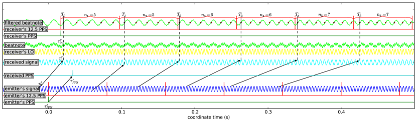
Figure 5: Both emitter’s and receiver’s signals are represented against coordinate time scale. Red dots on the filtered beatnote indicate zero crossings on ascending edge. $n_{m}$ is the number of red dots between two 12.5 PPS pulses. $T_{m-1}$ is the proper time of the first red dot in the same sequence. Propagation times are represented by black arrows. Here signal frequency is much lower than in reality, and Doppler effect is strongly magnified in order to show variation of $n_{m}$.

We explain here basic principles of the ground/space modems developed by TimeTech/Astrium for the ACES/PHARAO mission, that will be linked to the clocks and the antennas. This principle is illustrated on fig.5. At emitter and receiver are generated a PPS signal (one Pulse Per Second), a 12.5 PPS (one pulse every 80 ms, the period of measurements), and a periodic signal (either code at 100 MHz or carrier). Let $e$ be the emitter and $r$ the receiver. A PPS signal sent at local time $\tau_{\text{pps}}^{e}$ of the emitter is received at local time $\tau_{\text{pps}}^{r}$ of the receiver. Local time $\tau_{\text{pps}}^{r}$ is recorded by the modem for each received PPS.

When received, the periodic signal (blue) is mixed with a local oscillator (yellow) which frequency is not far from the received frequency, and filtered to obtain the low frequency part of the beatnote (green). The beatnote frequency is around 195 kHz for code and 729 kHz for carrier. The receiver modem records the time of the first ascending zero-phase of the beatnote signal after the 12.5 PPS signal. We call this observable $T_{m}$, where $m$ is the number of the 80 ms sequence. Finally, the modem counts the number of ascending zero-phase $n_{m}$ during sequence $m$.

$\tau_{\text{pps}}^{r}$, $T_{m}$, $n_{m}$ and $m$ are the basic observables of the modem, called TT observables, and are recorded for code and carrier signals. The modem internal clock is reset every 4 s. However, code observables can be linked to UTC time, which permits to solve the phase ambiguity between each passage for code observables.

III-A From TT to ST observables

Figure 6: Link between phase, emitter and receiver local times.

Let $\phi_{e}(\tau^{e})$ and $\phi_{r}(\tau^{r})$ be respectively the phase of emitted and received signals, changing with local time of emitter and receiver. Let’s consider two signals: one emitted at emitter local time $\tau^{e}_{0}$ and received at receiver local time $\tau^{r}_{0}$, and another one, emitted at $\tau^{e}_{1}$ and received at $\tau^{r}_{1}$ (see fig. 6). The phase increase between these two signals is equal at emitter and receiver:

$$\phi_{e}(\tau^{e}_{1})-\phi_{e}(\tau^{e}_{0})=\phi_{r}(\tau^{r}_{1})-\phi_{r}(\tau^{r}_{0}).$$ (21)

The received signal is mixed with a local oscillator signal such that the beatnote phase is:

$$\phi_{\text{b}}(\tau^{r})=\left\{\begin{array}[]{ll}\phi_{\text{L.O.}}(\tau^{r})-\phi_{r}(\tau^{r})&\text{(for code)}\\ \phi_{r}(\tau^{r})-\phi_{\text{L.O.}}(\tau^{r})&\text{\color[rgb]{1,0,0}(for carrier)}\end{array}\right.$$ (22)

Signs are different for code and carrier; we will write subsequent formulas in a compact way with the sign in black for code and red for carrier. We assume $\phi(\tau)=\omega\tau+\text{cst}$, where $\omega$ is the pulsation of the considered signal. Then, from eqs.(21) and (22) we deduce:

$$\tau^{e}_{1}-\tau^{e}_{0}=\dfrac{\omega_{\text{L.O.}}}{\omega_{e}}(\tau^{r}_{1}-\tau^{r}_{0})\stackrel{{\scriptstyle{\color[rgb]{1,0,0}+}}}{{-}}\dfrac{1}{\omega_{e}}(\phi_{\text{b}}(\tau^{r}_{1})-\phi_{\text{b}}(\tau^{r}_{0}))$$ (23)

We introduce the ST observable, which links local time of emission to local time of reception: $\Delta\tau^{r}(\tau^{r})=\tau^{e}-\tau^{r}$. From eq.(23) we get:

$$\begin{array}[]{ll}\Delta\tau^{r}_{1}(\tau^{r}_{1})-\Delta\tau^{r}_{0}(\tau^{r}_{0})=&\left(\dfrac{\omega_{\text{L.O.}}}{\omega_{e}}-1\right)(\tau^{r}_{1}-\tau^{r}_{0})\\[10.84006pt] &\stackrel{{\scriptstyle{\color[rgb]{1,0,0}+}}}{{-}}\dfrac{1}{\omega_{e}}(\phi_{\text{b}}(\tau^{r}_{1})-\phi_{\text{b}}(\tau^{r}_{0}))\end{array}$$ (24)

Let’s apply this formula to the MWL modem by introducing the TT obervables: $\tau^{r}_{0}=T_{m-1}$ and $\tau^{r}_{1}=T_{m}$. From definition of $T_{m}$ and $n_{m}$ observables we know that $\phi_{\text{b}}(T_{m})-\phi_{\text{b}}(T_{m-1})=2\pi n_{m}$. Then we deduce from eq.(24):

$$\begin{array}[]{ll}\Delta\tau^{r}_{m}(T_{m})=&\Delta\tau^{r}_{m-1}(T_{m-1})\\[10.84006pt] &+\left(\dfrac{\omega_{\text{L.O.}}}{\omega_{e}}-1\right)(T_{m}-T_{m-1})\\[10.84006pt] &\stackrel{{\scriptstyle{\color[rgb]{1,0,0}+}}}{{-}}\dfrac{2\pi n_{m}}{\omega_{e}}\end{array}$$ (25)

where $\Delta\tau^{r}_{m}$ is the ST observable corresponding to sequence $m$. This recursive formula allows to find all ST observables from TT observables, if the first term $\Delta\tau_{0}^{r}(T_{0})$ is known. We notice than in case of zero Doppler, the last two lines of the equation cancel, and the ST observable $\Delta\tau^{r}$ should be constant with local time.

Relative accuracy of ST observables during one passage of ISS is:

$$\begin{array}[]{lcl}\delta(\Delta\tau^{r}_{m})&\sim&\left|\dfrac{\omega_{\text{L.O.}}}{\omega_{e}}-1\right|\cdot\delta T_{m}\\[14.45377pt] &\sim&\left\{\begin{array}[]{ll}\frac{195~{}\text{kHz}}{100~{}\text{MHz}}\cdot 10~{}\text{ns}\sim 20~{}ps&\text{(code)}\\[7.22743pt] \frac{729~{}\text{kHz}}{13.5~{}\text{GHz}}\cdot 10~{}\text{ns}\sim 0.5~{}ps&\text{(carrier)}\end{array}\right.\end{array}$$

where accuracy of $T_{m}$ observables, $\delta T_{m}\sim 10$ ns, can be deduced from modem internal clock, which frequency is around $100$ MHz. However, $\delta T_{m}$ is underestimated here because other noise sources than the internal clock may count. The goal here is not to do a precise accuracy budget but rather get a lower limit.

III-B Initial term determination

What is the first term of the iterative series (25)? Our goal is to determine $\Delta\tau^{r}_{0}(T_{0})$ with an absolute accuracy $<100$ ps, which is required for ground-space time transfer. For frequency transfer, we should be able to bridge the gap between two passages with an accuracy depending on the duration between them, which can be read on fig.2 (e.g. 1.5 ps for two passages separated by one orbital period).

Let

$$\Delta\tau_{\text{pps}}^{r}(\tau_{\text{pps}}^{r})=\tau_{\text{pps}}^{e}-\tau_{\text{pps}}^{r}=\tau_{\text{ini}}^{r}-\tau_{\text{pps}}^{r}$$ (26)

be the ST observables linked to TT observables $\tau_{\text{pps}}^{r}$, and $\tau_{\text{ini}}^{r}$ be the receiver local time of generation of the PPS, which is by definition of the experiment equal to the local time of emission of the same PPS signal $\tau_{\text{pps}}^{e}$. As $\tau_{\text{pps}}^{e}$ can be guessed from a UTC tag, $\Delta\tau_{\text{pps}}^{r}(\tau_{\text{pps}}^{r})$ is known and can be linked to $\Delta\tau^{r}_{0}(\tau^{r}_{0})$ with the help of eq.(24):

$$\begin{array}[]{ll}\Delta\tau_{0}^{r}(\tau^{r}_{0})=&\Delta\tau_{\text{pps}}^{r}(\tau_{\text{pps}}^{r})+\left(\dfrac{\omega_{\text{L.O.}}}{\omega_{e}}-1\right)\left(\tau_{0}^{r}-\tau_{\text{pps}}^{r}\right)\\[10.84006pt] &-\dfrac{1}{\omega_{e}}(\Phi_{\text{b}}(\tau_{0}^{r})-\Phi_{\text{b}}(\tau_{\text{pps}}^{r}))\end{array}$$ (27)

From the values of $T_{m}$ and $n_{m}$ one can determine the beatnote phase at $\tau_{\text{pps}}^{r}$. The uncertainty in that determination is $\delta\Phi_{b}(\tau_{\text{pps}}^{r})\sim\omega_{b}\cdot\delta T_{m}\sim 0.012$ rad. The uncertainty of the two last terms on the rigth side of the equation is then $\sim 20$ ps, which is sufficient. However, $\Delta\tau_{\text{pps}}^{r}$ is known with the modem internal clock accuracy, i.e. $\delta(\Delta\tau_{\text{pps}}^{r})\sim 10$ ns. Even averaging on a complete data set is not sufficient, reaching $\sim 580$ ps accuracy with 300 points. Then we need a method to obtain a precise PPS observable.

III-B1 Precise PPS observable

the emitter PPS is phase coherent with the code phase and the receiver PPS is phase coherent with the local oscillator phase. Then we can use the internal counter and the code phase observables to follow the phase precisely and derive a more accurate pps observable that we call $\Delta\tau_{\text{ppps}}^{r}$.

The receiver local oscillator is phase coherent with the receiver PPS (it has a zero crossing at $\tau_{\text{ini}}^{r}$), then:

$$\Phi_{\text{L.O.}}(\tau_{\text{ini}}^{r})=2\pi N_{\text{L.O.}}$$ (28)

where $2N_{\text{L.O.}}$ is an integer. Similarly the emitted (and received) code is phase coherent with the emitted (received) PPS, so we have

$$\Phi_{e}(\tau_{\text{pps}}^{e})=\Phi_{r}(\tau_{\text{pps}}^{r})=2\pi N_{B}$$ (29)

where $N_{B}$ is an integer. Using eqs.(22), (26), (28) and (29) we obtain:

$$\Delta\tau_{\text{ppps}}^{r}(\tau_{\text{pps}}^{r})=\dfrac{1}{\omega_{\text{L.O.}}}\left(2\pi N-\phi_{\text{b}}(\tau_{\text{pps}}^{r})\right),$$ (30)

where $2N=2(N_{\text{L.O.}}-N_{B})$ is an integer. Provided we can determine the integer $2N$ exactly, the uncertainty on $\Delta\tau_{\text{ppps}}^{r}$ is $\delta\phi_{\text{b}}/\omega_{\text{L.O.}}\sim 20$ ps. The value of $N$ is determined by using the direct measurement $\Delta\tau_{\text{pps}}^{r}(\tau_{\text{pps}}^{r})$ in eq.(30) above:

$$N=\dfrac{1}{2\pi}\left(\omega_{\text{L.O.}}\Delta\tau_{\text{pps}}^{r}(\tau_{\text{pps}}^{r})+\Phi_{\text{b}}(\tau_{\text{pps}}^{r})\right)$$ (31)

Uncertainty of the second term in (31) is $\sim 0.012/(2\pi)\sim 2\cdot 10^{-3}$, therefore negligible. However, uncertainty of the first term is $\sim\omega_{\text{L.O.}}\cdot 10~{}\text{ns}/(2\pi)\sim 1$, which is insufficient. One solution is to average over all PPS measurements of a continuous passage, which should be sufficient for realistically useful passages (e.g. $>50$ s).

Finally using the precise PPS observable $\Delta\tau_{\text{ppps}}^{r}(\tau_{\text{pps}}^{r})$ calculated from eq.(30) in eq.(27) reaches the required accuracy for time transfer.

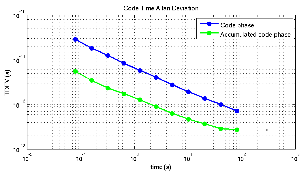
(a) Code observables

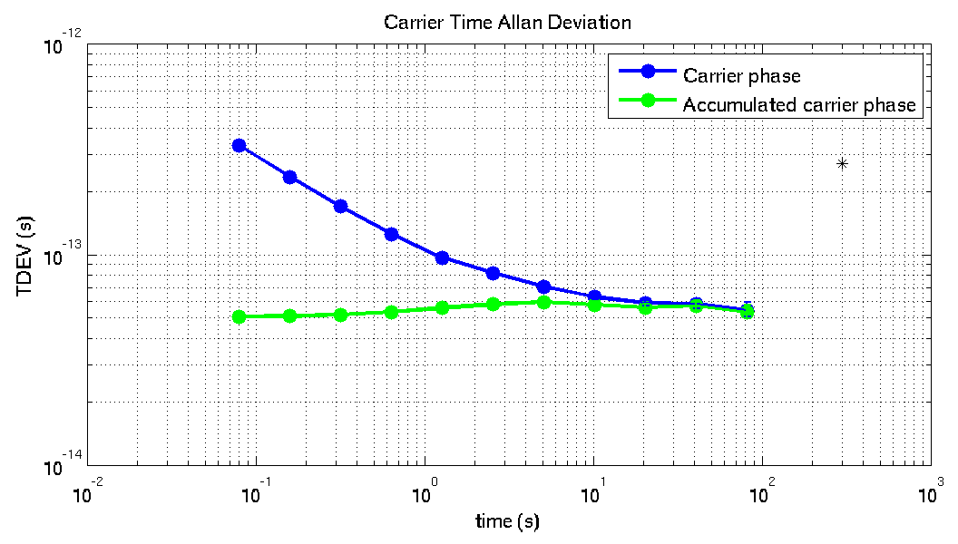
(b) Carrier observables

Figure 7: Short term stability (TDEV) of ST observables, derived from either code/carrier phase or accumulated code/carrier phase.

III-B2 Bridging the gap

to perform ground-space frequency comparisons on long term one needs to link observables from two different ISS passages. It is then necessary to determine precisely the time elapsed from one passage to another thanks to the TT observables. Let’s call $\Delta\tau_{0}(\tau_{0})$ and $\Delta\tau_{0}^{\prime}(\tau^{\prime}_{0})$ the initial terms of two different passages (in this section we omit the $r$ indices on ST observables $\Delta\tau^{r}$ and on local time $\tau^{r}$). The error on their absolute determination is $\sim 20$ ps. However we want to reach $\delta\left(\Delta\tau^{\prime}_{0}(\tau^{\prime}_{0})-\Delta\tau_{0}(\tau_{0})\right)\lesssim x$, where $x$ is a specification that depends on the duration separating the two passages and can be read from fig.2 (e.g. 1.5 ps for one orbital period separation). From eq.(24) we deduce:

$$\begin{array}[]{ll}\phi_{\text{b}}(\tau^{\prime}_{0})-\phi_{\text{b}}(\tau_{0})=&-\omega_{e}(\Delta\tau^{\prime}_{0}(\tau^{\prime}_{0})-\Delta\tau_{0}(\tau_{0}))\\[7.22743pt] &+\left(\omega_{\text{L.O.}}-\omega_{e}\right)(\tau^{\prime}_{0}-\tau_{0})\end{array}$$ (32)

Moreover, we know that $\phi_{\text{b}}(\tau^{\prime}_{0})-\phi_{\text{b}}(\tau_{0})=2\pi N_{g}$, where $N_{g}$ is an unknown integer. We deduce that:

$$\begin{array}[]{ll}N_{g}=\dfrac{1}{2\pi}&(-\omega_{e}(\Delta\tau^{\prime}_{0}(\tau^{\prime}_{0})-\Delta\tau_{0}(\tau_{0}))\\ &+\left(\omega_{\text{L.O.}}-\omega_{r}\right)(\tau^{\prime}_{0}-\tau_{0}))\end{array}$$ (33)

It can be shown that the accuracies of the different terms in this equation are sufficient to determine $N_{g}$ whithout ambiguity. Then we deduce:

$$\Delta\tau^{\prime}_{0}(\tau^{\prime}_{0})-\Delta\tau_{0}(\tau_{0})=\left(\dfrac{\omega_{\text{L.O.}}}{\omega_{e}}-1\right)(\tau^{\prime}_{0}-\tau_{0})-\dfrac{2\pi N_{g}}{\omega_{e}}$$ (34)

This equation links ST observables from two passages to $\sim$ 20 ps, which is not sufficient as can be seen from fig.2. Using several pairs of code observables to determine this quantity will not increase the accuracy, as the error for each data pairs will be correlated. Two solutions can be envisioned. One can use carrier phase observables. However, it remains to be seen if the phase ambiguity (integer $N_{g}$) can be solved for carrier phase. This will be studied in another article. Second solution would be to use another observable from the MWL modem: the accumulated phase $T^{\text{acc}}_{m}$, which is the sum of all dates of ascending zero-phase during sequence $m$.

In fig.7 is shown the short-term stability of ST observables, calculated either using $T_{m}$ or $T^{\text{acc}}_{m}$ observables, for code (fig.7(a)) and carrier (fig.7(b)). It can be seen that using $T^{\text{acc}}_{m}$ observables increases measurements accuracy. However, code accuracy is still not sufficient to bridge the gap between two passages: we assume that ST observables uncertainty is $\delta(\Delta\tau)\sim 3\times\text{TDEV}_{0}$, where $\text{TDEV}_{0}$ is the Time deviation for $\tau=0.08$ s, the period of measurements. Then, from fig. 7(a), $\delta(\Delta\tau)\sim 90$ ps for code phase and $\delta(\Delta\tau)\sim 18$ ps for accumulated code phase. This is not sufficient to bridge any gap. From fig. 7(b) we deduce $\delta(\Delta\tau)\sim 0.9$ ps for carrier phase and $\delta(\Delta\tau)\sim 0.15$ ps for accumulated code phase. Any of these two observable is sufficient to bridge a gap of 30 mn or larger. It remains to be seen how to solve the phase ambiguity for carrier phase, which will be studied in another article.

IV Simulation and data analysis

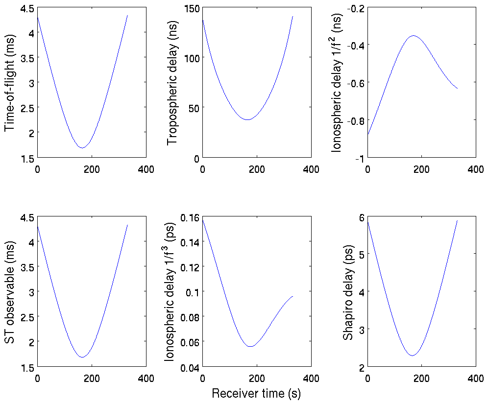
Figure 8: Contribution of atmospheric and Shapiro delays in the simulated time-of-fligth of the $f_{1}$ signal.

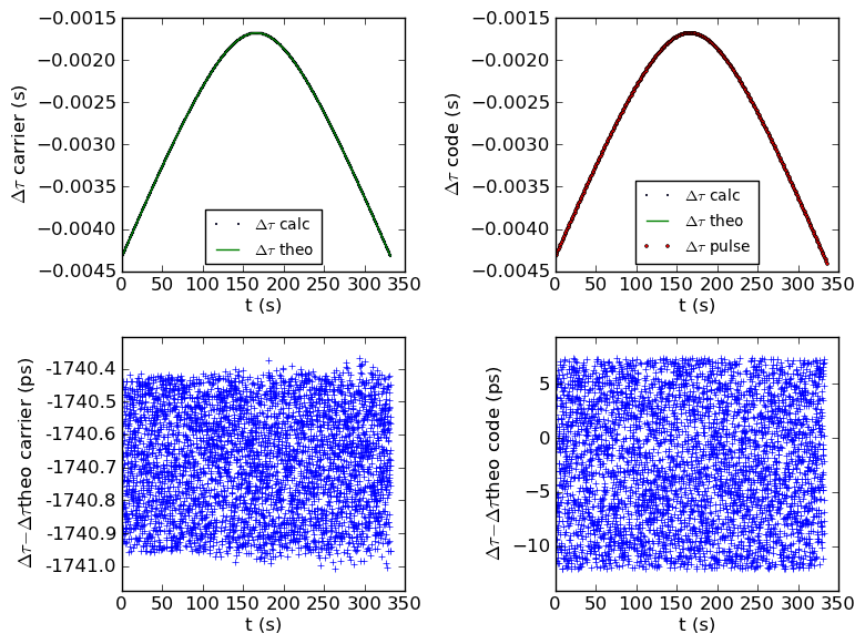
Figure 9: Pre-processing software: comparison between ST observables calculated from simulated TT observables, and theoretical ST observables, for carrier (left) and code (right).

The SYRTE team writes an independant data analysis software, in order to make the most of the ACES/PHARAO mission data. This software is written in Python language. In order to test it, we wrote a simulation that generates (noisy) TT observables, as well as theoretical ST observables. This simulation is written in Matlab language, and is as much as possible independant from the data analysis software.

IV-A Simulation

The simulation takes as input orbitography of the ISS and one Ground Station (GS) in a Celestial Reference System. From orbitography files it simulates the proper times given by ISS and GS clocks, and the time transfer between these two clocks, using a modelization of the MWL. Observables are given in terms of TT and ST observables. Moreover, theoretical values of the scientific products are given in order to test the data analysis software.

In fig.8 we have plotted different contributions included in the signal time-of-flight of signal $f_{1}\simeq 13.5$ GHz. Minimum elevation of ISS is taken as 10˚, and atmospheric parameters are temperature $T=298$ K, pressure $p=1$ bar and water vapor pressure $e=0.5$ bar. A sinusoidal variation is added to atmospheric parameters, with a period of 24 hours, and a Chapman layer model is used to calculate the STEC.

Tropospheric delay is dominant in the time-of-flight, with a value of several 10 ns. We used here a Saastamoinen model, which is not really reliable at low elevation of ISS. The dispersive part of troposphere has not been taken into account, and it remains to be seen if this is necessary. Ionosphere is dispersive such taht the ionospheric delay can be separated in two contributions: an effect that scales with $1/f^{2}$ and one that scales with $1/f^{3}$ (see eqs.(15)-(16)). The second order contribution is around 1 ns and the third contribution around 0.1 ps, below mission accuracy. However these effects are much larger for the $f_{3}=2.25$ GHz signal: around 40 ns for second order term and 20 ps for third order term. Then third order terms cannot be ignored. Finally the Shapiro delay of several ps is sligthly over the required accuracy.

IV-B Data analysis

An independant pre-processing software has been written, using equations from sec.III. It takes TT observables from the simulation, transform them to ST observables and compare the result to the theoretical ST observables coming from the simulation. One example can be seen on fig.9. It can be seen that ST observables are well recovered, with a noise which is coherent with previous estimations. However here the noise is underestimated because all noise sources has not be included (only the modem internal clock noise). The absolute value of the ST code observable is found thanks to the method of the initial term determination, with an uncertainty less than 20 ps (explaining why the data cloud is not centered on 0). The phase ambiguity for carrier observable has not been solved, explaining the constant bias between the recovered and the theoretical ST carrier observables.

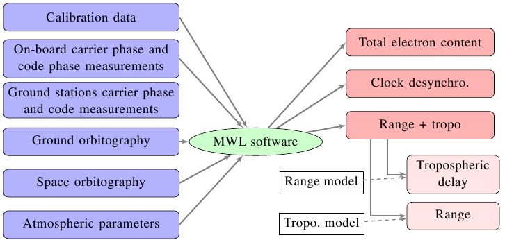
Figure 10: Full data analysis software: illustration of inputs and outputs.

The full data analysis software is being written but not finished yet. We explain its basic principle on fig.10. A special care is taken for file naming, data classifying, file formats and conventions. Indeed many data from several different sources will have to be used and these issues can be critical. The software design has been build in a modular way, and now most of the building blocks are written.

V Conclusion

We have written a theoretical description of one-way and two-way satellite time and frequency transfer and developed a model of the Micro-Wave Link in the frame of the ACES/PHARAO mission. This description has been used to write a data analysis software and a simulation to test it. The simulation is written in its first version, and used to assess our pre-proceesing software. The design of the data analysis software has been done in a modular way, and most of the building blocks are ready.

Several questions remains: how to solve the phase ambiguity for the carrier observable, what is the dispersive effect of the troposphere?

References

[1]
L. Cacciapuoti and C. Salomon, “Aces mission objectives and scientific
requirements,” ESA, Tech. Rep., 2010, aCE-ESA-TN-001, Issue 3 Rev 0.
[2]
L. Duchayne, F. Mercier, and P. Wolf, “Orbit determination for next
generation space clocks,” Astronomy and Astrophysics, vol. 504, pp.
653–661, Sept. 2009.
[3]
L. Duchayne, “Transfert de temps de haute performance : le lien micro-onde de
la mission ACES,” Ph.D. dissertation, Observatoire de Paris, France, 2008.
[Online]. Available: http://tel.archives-ouvertes.fr/tel-00349882/fr/