Driving kinetically constrained models into non-equilibrium steady states:
Structural and slow transport properties

Abstract

Complex fluids in shear flow and biased dynamics in crowded environments exhibit counterintuitive features which are difficult to address both at a theoretical level and by molecular dynamic simulations. To understand some of these features we study a schematic model of a highly viscous liquid, the two-dimensional Kob-Andersen kinetically constrained model, driven into non-equilibrium steady states by a uniform non-Hamiltonian force. We present a detailed numerical analysis of the microscopic behavior of the model, including transversal and longitudinal spatial correlations and dynamic heterogeneities. In particular, we show that at high particle density the transition from positive to negative resistance regimes in the current vs field relation can be explained via the emergence of nontrivial structures that intermittently trap the particles and slow down the dynamics. We relate such spatial structures to the current vs field relation in the different transport regimes.

I Introduction

Slow relaxation and anomalous diffusion are common features of disordered systems. In particular, viscous liquids and highly packed matter show dynamically arrested states (the glassy and the jammed state respectively) characterized by steeply increasing relaxation times and spatially heterogeneous and intermittent dynamics DH ; heterogeneities . Similar behavior has been also observed in sheared complex fluids and dense granular materials larson ; fragile ; jamming , though in these latter cases it is much more difficult to understand as it requires a full dynamical description, due to the absence of a Boltzmann-Gibbs framework.

The microscopic origin for these peculiar dynamically arrested states has been the subject of many studies. It has been shown that gels, colloids, and supercooled liquids generally exhibit rare mobility regions, and that an increase of mobility due to local relaxation events facilitates the dynamics, allowing other regions to participate cooperatively. Such facilitation mechanism has been supposed to be one of the reasons underlying the slow dynamics and is at the origin of a vast class of models called Kinetically Constrained Models (KCM), see Ritort-Sollich ; kcms for reviews.

These models are very simple from a thermodynamic point of view as they do not rely on any specific interaction potentials, but rather on particular dynamic evolution rules. They can be implemented under two closely related forms: facilitated spin systems or kinetically constrained lattice gases. In the first case, spins represent mobile (or active) regions that flip between two or more states depending on the status of the nearest neighbors, which can either facilitate or forbid some spin flip. In the second case, the particle dynamics on a lattice follows some specific kinetic rule facilitating or suppressing some particle moves depending on the nearby local particle density. In the spin case, the control parameter is the temperature defining the density of excited states, while in the second case the particle density (i.e the packing fraction) plays a central role. Both dynamic evolution rules aim at simulating the cage effect due to the steric hindrance among particles or spins belonging to the same dense region.

We consider here a specific case of the latter class of models, the two-dimensional (2D) Kob-Andersen model with an externally applied field, as introduced in Ref. sellitto .

In ref. sellitto , it has been shown by numerical simulation that at high density, the model features a crossover from a flowing (positive resistance) regime at a small field to a negative differential resistance regime at a larger field. The latter regime is accompanied by unusual transport properties, including non-monotonic field dependence of the structural relaxation time and rheological-like behavior sellitto . Notably, the asymptotic large-deviation limit in which the fluctuation relation holds is hardly attained on the simulation timescale sellitto2 ; TurciPitard . In ref. TurciPitard , the anomalous space-time behavior of the system has been quantified by providing a description in terms of a field dependent dynamical transition between a flowing and blocked phase with the use of the language of the thermodynamic of histories. This formalism has been used to evidence such a dynamical phase transition in undriven glassy systems histories . The present paper is an extended version of Refs. sellitto ; TurciPitard in which numerical simulation results (some of which were previously announced only) are now fully reported and are better understood in terms of a theoretical approach. In particular, we give a microscopic description in configuration space of the two transport regimes and describe the nontrivial dynamical heterogeneities induced by the driving force. The paper is organized as follows: in section II we present the description of the model, with the characterization of the relationship between the current, the density of particles and the driving field in section III; in section IV we discuss the role of heterogeneities; in section V we compute global space correlation functions and in section VI we relate the microscopic structure (traps and domain walls) to the current.

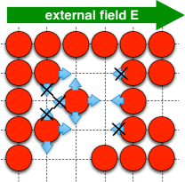
Figure 1: (color online) Scheme of the model rules and the role of the kinetic constraints: particles (red) can move and occupy empty sites if they have at least 2 empty neighbors before and after the move. The external field is uniform and biases the movement of the particles from left to right reducing the probability of backward moves.

II The model

We consider the model proposed by one of us in Ref. sellitto . It can be viewed either as the kinetically constrained version of a $2D$ Asymmetric Simple Exclusion Process (ASEP) or as the Kob-Andersen model in presence of an external (non Hamiltonian) field. In the absence of drive the model has been largely studied; see, e.g., Refs. KoAn ; KuPeSe ; FrMuPa ; ToBiFi ; MaPi ; ChSaKo ; PaPiCaCo . We take a $2D$ regular square lattice of size $L\times L$ with periodic boundary conditions, in which the particle density $\rho$ is a conserved parameter. The $N=\rho L^{2}$ particles are initially put at random on the lattice, and an external field $E$ is applied along the horizontal direction, from left to right, as illustrated in Fig. 1. In this situation, the probability that a particle moves against the field is $p_{back}={e}^{-E/k_{\scriptscriptstyle\rm B}T}$, while each other direction is equiprobable. We shall set the Boltzmann constant $k_{\scriptscriptstyle\rm B}$ to 1 throughout the paper and absorb the temperature $T$ in the field definition, as the system we consider is purely athermal and no additional energetic interaction among particles is considered.

The model dynamics is fully described by the following steps:

1. A particle is chosen at random uniformly.

2. The particle attempts to move along one of the four possible directions, by choosing one of its nearest neighbors site randomly with equal probability ($1/4$).

3. The particle motion to the randomly chosen site takes place only if the site is empty and the particle has at least 2 empty neighbors before and after the move. This latter condition is the so-called kinetic constraint.

4. If the previous condition is satisfied, the particle always moves provided that motion does not occur against the applied field; otherwise, if the particle attempts to move against the field, the motion occurs only if a random number uniformly chosen in the range $[0,1]$ is less than ${e}^{-E}$. This step is known as the Metropolis rule.

We measure time in unit of Monte Carlo sweep, corresponding to the random sequential update of the state of each particle on average. Using a Metropolis-like algorithm allows one to make contact with some standard results found in the literature on the ASEP and the Totally Asymmetric Simple Exclusion process (TASEP), which are recovered here in the absence of kinetic constraints and infinite field. The Metropolis choice maximizes the number of moves in the field direction, because every attempt to move a particle along the field in the unit time and by a lattice spacing is always accepted. It is however not evident a priori that the transport properties are qualitatively independent from the chosen evolution rule. Therefore we have implemented, as an alternative to the Metropolis algorithm, a Glauber-type dynamics according to which the probability to move a particle against or along the applied field depends on whether the random number, uniformly chosen in the range $[0,1]$, is less or larger than $(1+{e}^{E})^{-1}$, respectively. Results are pretty robust and confirm our expectation that the transport properties we found are generic: they are essentially due to the presence of kinetic constraints that cannot be violated, no matter the choice of transition probabilities. Finally, we notice that the local time reversibility of the microscopic dynamics is satisfied.

III Transport regimes: current vs field relation

The central quantity we focus on in this section is the particle current, $J$, which is defined as the number of jumps in the field direction minus the one in the opposite direction per lattice site and per unit time. It allows a first macroscopic characterization of the different transport regimes present in the system. We generally observe the existence of a threshold density $\rho_{\scriptscriptstyle\rm c}\simeq 0.79$, below which the current vs field relation is monotonic and above which the current exhibits a crossover from a linear (ohmic) regime to a negative differential resistance (non ohmic) regime at increasing field; see figs. 2 and 3.

III.1 Low density regime

In the small density regime, we expect that transport is weakly influenced by the presence of kinetic constraints: indeed numerical simulations show that the current vs field relation has a form much similar to the ASEP asep ; see Fig. 2. So we can set:

$$J(\rho,E)=A\,\frac{1}{4}\rho(1-\rho)(1-{e}^{-E}),$$ (1)

with the pre-factor $A$ accounting for a further possible dependence on $\rho$ and $E$ ascribed to the constrained dynamics. We can consider two limiting cases. In the absence of constraints, the pre-factor $A$ must be 1, consistently with the ASEP. When the field becomes very large, the current saturates to a finite value, which for the standard TASEP is $J_{\rm\scriptstyle sat}\sim\rho(1-\rho)$. When increasing the particles density the effect of the constraints is to reduce the number of accessible paths in the configuration space and to slow down the dynamics so that the current is smaller than what expected in the unconstrained case. Interestingly enough, even though the value of the pre-factor $A$ decreases continuously with increasing $\rho$, it does not depend on the applied field, so that Eq. (1) takes the same scaling form in the whole $\rho<\rho_{\scriptscriptstyle\rm c}\simeq 0.79$ regime, as far as its field dependence is concerned; see Fig. 2(b).

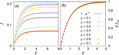
Figure 2: (color online) (a) Current $J$ vs field $E$ relation for subcritical densities, $\rho<\rho_{\scriptscriptstyle\rm c}\simeq 0.79$. The system size is $L^{2}=50^{2}$. The current is a monotonic function of the field, saturating at large field. Its behavior is qualitatively similar to the ASEP on a 2D square lattice. (b) The density dependence of the current vs field relation can be easily accounted for by rescaling $J(E)$ with the saturation current $J_{\rm\scriptstyle sat}(\rho)$. The current ratio $J/J_{\rm\scriptstyle sat}$ is exactly equal to the difference between forward and backward transition probabilities, $1-{e}^{-E}$.

The similarity between the two behaviors - with and without constraints - suggests that the density dependence of $A(\rho)$ can be estimated by the means of a mean-field approach that neglects the role of two-point and higher-order correlations. This approximation allows us to quantify the value of $A(\rho)$, writing

$$A(\rho)=(1-\rho^{3})^{2},$$ (2)

which implies

$$J(\rho,E)=\frac{1}{4}(1-{e}^{-E})\rho(1-\rho)(1-\rho^{3})^{2}.$$ (3)

The analysis of this expression is straightforward: the factor $1/4$ accounts for the four possible directions of motion on the $2D$ square lattice; the term $1-{e}^{-E}$ is the difference between the forward and backward transition probabilities; the product $\rho(1-\rho)$ gives the probability to find a particle on a certain site of the lattice with a nearby hole, if all correlations are neglected; in this approximation, the last term $(1-\rho^{3})^{2}$ simply accounts for the kinetic constraint: It reads as the probability to have at least two empty neighbors (which is equal to that one of not having three occupied neighbors), and is counted twice because of the local microscopic reversibility of the kinetic rule. In the strong field limit, $E\to\infty$, the current saturates to the value

$$J_{\rm\scriptstyle sat}(\rho)=\frac{1}{4}\rho(1-\rho)(1-\rho^{3})^{2}$$ (4)

As shown in Fig. 3(a), the mean-field approximation for the saturation current works well for small densities, suggesting the higher order correlations are negligible in that regime. When the density of particles increases, larger and larger correlations appear and above a certain density the mean field approach breaks down.

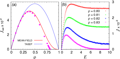
Figure 3: (color online) (a) The current as a function of the density for our model with the kinetic constraint in the limit of very strong fields. The peak is at $\rho\approx 0.4$ while for the classical TASEP (blue dashed line) the peak is at $\rho=0.5$. The mean-field formula (3) (red full line) shows a good qualitative agreement that becomes quantitative at densities below the peak value. (b) The most surprising property of the model: at high densities, $\rho>\rho_{\scriptscriptstyle\rm c}\simeq 0.79$, the simulations provide a current-field relation which is non-monotonic, as discussed in Ref. sellitto . Simulation data at $\rho>\rho_{\scriptscriptstyle\rm c}$ are obtained by using systems of size $L^{2}=400^{2}$.

Notice that in spite of the local microscopic time-reversibility of the kinetic rule and particle-hole symmetry, the interplay of the driving force and the kinetic constraints leads, in the limit of very strong fields, to an asymmetric current vs density relation as shown in Fig. 3(a). The emergence of global particle-hole broken symmetry can be understood as follows: the two limit situations where only one particle is present on the lattice and where there is only one hole do not lead to the same current: the first case has a finite current $J=\frac{1}{4}(1-{e}^{-E})/L^{2}$ while in the second case the current is strictly zero, due to the caging rules. One can compare the constrained model result at strong field with the TASEP, where the current is given by a parabola peaked in $\rho=0.5$. On the contrary, the constrained model is peaked around a smaller density ($\approx 0.4$) and shows an almost zero current region at particle density near 1.

III.2 High-density regime

At density above $\rho_{\scriptscriptstyle\rm c}$, see Fig. 3.(b), the non-monotonic behavior of $J(E)$ emerges as the signature of extra mechanisms producing a more complex transport dynamics. Such non-monotonic behavior is more and more pronounced with increasing density and is related to the growth of several orders of magnitude of the relaxation times of the system sellitto . At such high densities one can distinguish between two dynamical regimes: a positive resistance regime, where the current grows linearly with the field, and a negative resistance one, where the increase of the field corresponds to a decrease in the current, see Fig. 3.(b). The occurrence of non-monotonic transport can be qualitatively understood as a consequence of the decreasing probability of backword motion: at high density and increasing field, the particle rearrangements needed to remove obstruction to the flow, require more and more particle moves against, or normal to, the field direction, and this leads to a flow reduction. In particular, three distinct behaviors can be considered, as discussed in Ref. sellitto : (I) $J_{\rm\scriptstyle sat}$ is finite; (II) $J_{\rm\scriptstyle sat}$ is vanishingly small, if not zero; and (III) $J(E)$ vanishes above a finite driving force, $E>E_{\rm\scriptstyle c}$. Numerical results suggest that regime I occurs in the range $\rho_{\scriptscriptstyle\rm c}<\rho<0.83$ while regime II appears at a higher density. The existence of the jamming regime III cannot be obviously ascertained due to the strong finite-size effects related to bootstrap percolation. The characterization of these effects is notoriously difficult and so this jamming regime will not be discussed here. Rather, the main subject of this work will be the crossover between the linear and the non-monotonic transport regimes for a moderately large field and not too high particle densities.

IV Space and time heterogeneities

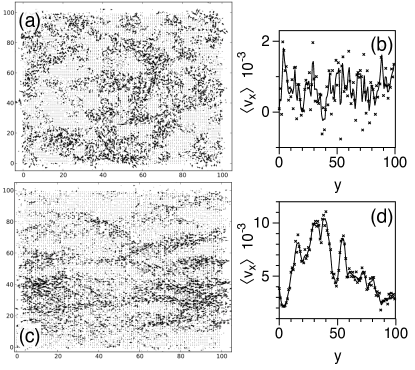
Figure 4: Average velocity field for an $L=100$ system at density $\rho=0.80$, with $E$ oriented left-to-right. In the top panels (a) and (b) the system is in the linear regime, $E=0.1$, while in the bottom panels (c) and (d) the system is in the negative differential resistance regime, $E=2.8$. The time window considered for the evaluation of the average speed is $t_{w}\approx 1\tau_{\scriptscriptstyle\rm rel}$. At small fields the dynamics is homogeneous, while in the negative resistance regime, shear bands appear. The boxes (b) and (d) represent the longitudinal projections of the velocity vectors averaged over each horizontal line of particles as a function of the transversal coordinate $y$.

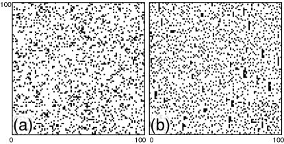
Figure 5: Snapshots of two steady-state configurations with particles (white) and holes (black) for a system of size $L=100$ and $\rho=0.82$ at (a) $E=0$ and (b) $E=5$ with $E$ being in the horizontal direction (left to right). One can notice the vertical (transversal to the field) structures arising in the strong field case (b).

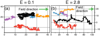
Figure 6: (color oline) Some examples of real space particle trajectories of equal duration $\tau=10^{4}$ in the two current regimes for a system of density $\rho=0.80$: (a) at small fields, $E=0.1$, and (b) large fields, $E=2.8$, corresponding to a negative resistance behavior. One can observe the mainly diffusive, brownian behavior (a) vs the directed behavior (b) where many steps are spent in wandering moves in the transversal direction. Each arrow corresponds to a directed step and the axes are in lattice spacing units.

The previous analysis suggests that the increase of the density beyond the critical value $\rho_{\scriptscriptstyle\rm c}$ corresponds to the switch between two qualitatively different transport regimes. The first step for the description of the high density regime is to analyze the configuration space, looking for a direct relationship between the non-monotonic behavior of $J(E)$ and changes in the typical arrangements of the particles, similarly to what has been done for other one-dimensional (1D) or 2D models (see, for example, JKGC ).

By the means of direct inspection, one can observe that the increase of the field leads to a transversal symmetry breaking in configuration space: not only do particles form longitudinal flowing bands along the field direction (see figure 4), but one can already visualize emerging structures composed by blocked and empty regions, inducing an intermittent dynamics for particles (fig. 5). Particles are trapped for very long times, wandering diffusively in the transversal direction, and occasionally make a fully directed jump in the field direction (fig. 6): such a behavior is responsible for the anomalous diffusion observed in previous works sellitto .

The inhomogeneities in the dynamics start to appear when the $J(E)$ peak is crossed and correspond to a coexistence between blocked and mobile trajectories. The average velocity field over time windows below the relaxation time of the system allows for a proper representation (fig. 4). Longitudinal bands of different mobility can be seen at large fields, while at small fields the spatial distribution of the velocity vectors is homogenous. In analogy with what is observed for sheared systems (i.e., shearbands ), we can call such structures shear bands. Nonetheless, these bands are not localized within the system, but have an intermittent and transient nature since the system is homogeneous if averaged over sufficiently long times. During the evolution, all the particles belong both to active and inactive bands.

V Anisotropic space correlations

Since the driven dynamics is obviously non-isotropic, we investigate here several measures of spatial anisotropy, namely, transversal and longitudinal persistence, dynamic susceptibility, two-point correlations, and the van Hove intermediate self-scattering function.

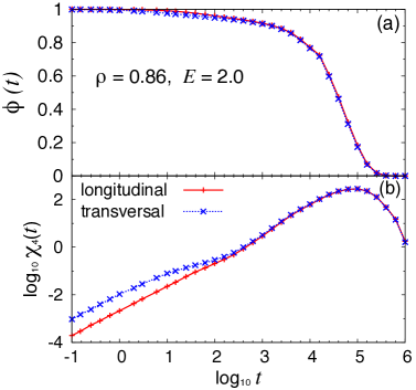
Figure 7: (color online) (a) Transversal ($\times$) and longitudinal (+) persistence, $\phi(t)$, vs time, $t$, for particle density $\rho=0.86$ and applied field $E=2.0$, corresponding to the negative differential resistance regime. Square lattice of linear size $L=500$. (b) transversal and longitudinal persistence fluctuations, $\chi_{4}$, for $\rho=0.86$ and $E=2.0$. Square lattice of linear size $L=100$.

V.1 Persistence and dynamic susceptibility

It is customary to characterize the dynamics of kinetically constrained systems by the persistence function, $\phi(t)$, i.e., the probability that a particle has never moved between times $0$ and $t$, whose field and density dependence have previously been discussed in Ref. sellitto . The long-time limit of $\phi(t)$ represents the fraction of particles that never moved, i.e., the fraction of permanently blocked particles. An asymptotic finite value of $\phi(t)$, therefore, signals a transition to a dynamically broken ergodicity regime. In our anisotropic system, we obviously need to distinguish between transversal and longitudinal particle motion leading to the definition of $\phi_{\scriptscriptstyle\rm T}(t)$ and $\phi_{\scriptscriptstyle\rm L}(t)$.

We find that the difference between longitudinal and transversal persistence functions is not sizable at a small field, and tiny at larger fields. In particular, it is only apparent in the early stage of relaxation of the large field regime. This suggests that there are no long-lived correlated structures but rather the continuous creation and destruction of spatially extended defects facilitating particle transport. Clearly, since persistence is a global, time-integrated quantity, it cannot represent an accurate probe of dynamic anisotropy on short-time scales. A slightly better characterization is provided by the dynamic susceptibility, which is generally defined as mean-square fluctuations of persistence

$$\chi_{4}(t)=N\left(\langle\phi^{2}(t)\rangle-\langle\phi(t)\rangle^{2}\right).$$ (5)

In Fig. 7 we plot the transversal and longitudinal component of persistence fluctuations. Differences between the two components are now more clearly visible at early times, and suggest the formation of short-lived correlated structures in the transversal direction. On a longer timescale the two susceptibility components show similar behavior: both the peaks position and the peaks height coincide, so that the behavior of the relaxation time as measured from the susceptibility peaks remains essentially unchanged.

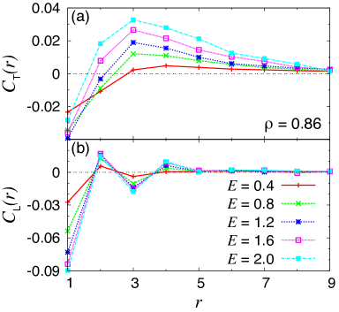
Figure 8: (color online) (a) Transversal and (b) longitudinal two-point correlation functions for $\rho=0.86$ for several applied fields $E$. Square lattice of linear size $L=500$.

V.2 Two-point correlation

To better quantify the anisotropy of dynamics we investigate here the behavior of a two-point correlation function at various values of density and driving field. The two-point correlation $C({\bf r})$ function is a measure of the spatial correlation of two particles at distance ${\bf r}$, and is defined here as

$$C({\bf r})=\frac{\left[\langle n_{\bf r+r_{0}}n_{\bf r_{0}}\rangle\right]_{\bf r_{0}}-\rho^{2}}{\rho(1-\rho)},$$ (6)

where the square brackets denote a spatial average and $n_{\bf r}=0,1$ are the usual lattice-gas occupation variables. In fig. 8 we show the transversal, $C_{\scriptscriptstyle\rm T}({\bf r})$, and the longitudinal, $C_{\scriptscriptstyle\rm L}({\bf r})$, two-point correlation functions in the non-equilibrium steady state.

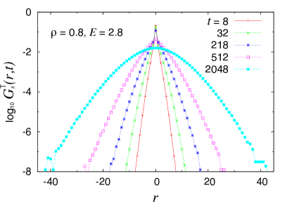
Figure 9: (color online) Transversal part of van Hove self correlation function at particle density $\rho=0.8$ and field $E=2.8$ (negative resistance regime). The system consists of a square lattice of linear size $L=50$.

In spite of the effective hard-core-like repulsion generated by kinetic constraints, we see that there is actually a medium short-range attractive-like interaction in the transversal direction to the applied force [fig. 8(a)]. The increased correlation between two nearby particles at a distance $r$, especially in the transversal direction, can be qualitatively explained as a purely dynamic effect, which arises from the fact that at large density and large applied field, any particle needs first to move either backward or transversally to the field direction in order to proceed forward. This effect is more and more pronounced as the density and the applied field increase. The interplay of kinetic constraints and driving force thus generally enhances the clustering of particles and appears to be akin to a transversal static short-range attraction. In the longitudinal direction instead we observe a short-range oscillatory behavior typical of liquids [fig. 8(b)]. These features can be linked to the different spatial structures that actually exist in the transversal and the longitudinal direction: we describe and discuss this in section VI.

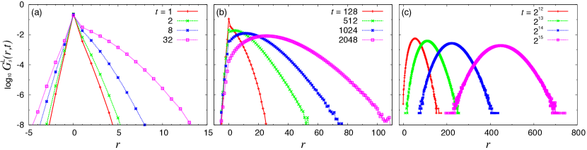
Figure 10: (color online) Longitudinal part of van Hove self-correlation function $G_{s}(r,t)$ vs position $r$ at time $t$, particle density $\rho=0.8$, and field $E=2.8$ (negative resistance regime) for a system of linear size $L=50$. There is long-lived asymmetry induced by the interplay of external drift and kinetic constraints. The exponential tails observed at short times eventually become more and more Gaussian at longer times.

V.3 van Hove self-correlation function

The van Hove self correlation function $G_{s}(r,t)$, quantifying the probability that a particle makes a displacement of size $r$ over a time interval $t$, is defined as

$$G_{s}(r,t)=\frac{1}{N}\sum_{i=1}^{N}\left\langle\delta(|{\bf r}_{i}(t)-{\bf r}_{i}(0)|-r)\right\rangle$$ (7)

where the delta is the Kronecker delta function. When the motion of particles is diffusive the van Hove function takes a Gaussian form. Deviations from the Gaussian behavior have been observed in a variety of glassy systems. Typically, one finds a crossover from an exponential decay at short-time, which is suggestive of dynamic heterogeneities (some particles move faster than others) to a Gaussian, normal diffusive behavior at large time - see Figs. 10 and 9. Consistently with other studies of relaxational glassy dynamics Chaudhuri ; Stariolo , we find a similar behavior in the particle transversal motion of our system. The latter, indeed can be assimilated to an equilibrium subsystem as there is no violation of detailed balance in the transversal direction. Interestingly, in the longitudinal direction, instead, we observe an asymmetric distribution of particle motion at early times, with Gaussian behavior slowly recovered at late times. The origin of the asymmetry in the distribution is due to the interplay between the drift caused by the field and the presence of kinetic constraints hindering crowded motion especially in the backward direction (against the field). The tail on the left side stays exponential over a longer time than on the right side, because the backward events leading to larger structural rearrangements are more rare. At large enough field backward motion is so obstructed that the time it takes to approach the Gaussian behavior can be exceedingly long to be observed.

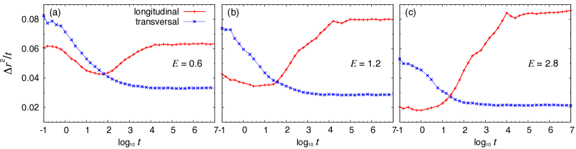
Figure 11: (color online) Time averaged longitudinal (+) and transversal ($\times$) mean-square displacement $\Delta r^{2}/t$ for a square lattice of linear size $L=50$. The normal diffusive behavior $\Delta r^{2}\sim t$ corresponds to horizontal lines; negative (positive) slope corresponds to sub (super) diffusion regime, respectively.

V.4 Mean-square displacement: anomalous diffusion

The differences we observed in the longitudinal and transversal motion are further confirmed by the analysis of the mean-square displacement. In fig. 11 we show the transversal and longitudinal mean-square displacements as a function of time. In the early stage of the dynamics, we see a sub-diffusive behavior in the transversal direction which correspond to the slow structural rearrangements of small size. This regime shrinks at large field and the asymptotic normal diffusion behavior is characterized by a diffusion coefficient that decreases with the applied field. In the longitudinal direction, the initial short-time sub-diffusion is followed by an intermediate super-diffusive behavior whose lifetime increases with the applied field. It corresponds to the regime in which the longitudinal van Hove function is strongly asymmetric and there are longitudinal particle rearrangements of large size. Normal diffusion is recovered at late times and, perhaps surprisingly, it is enhanced by increasing the applied field. We will show later that anisotropies are crucial for the dynamics and can be described microscopically in terms of intermittent creation and destruction of domain walls.

VI Traps and domain walls

Although the space and time averaged macroscopic observables exhibit several interesting features observed in more realistic systems, they shed little light on the microscopic mechanisms responsible for the blocking phase. Several transport problems showing reduced mobility involve the presence of localization and trapping of the carriers JKGC ; shlovskii ; bouchaud-anom-diff ; bouchaud-traps ; Dhar-Dietrich . In these problems anomalous diffusion and broad distributions of the waiting times of the particles are often found along with a non-monotonous dependence of the particle current on the external forcing or bias. In this context, we want to relate $J(E)$ to some specific properties of the domain walls or “walls of holes” that act as trapping and blocking regions for the dynamics.

We have quantified these regions by the average value of their longitudinal $w_{l}$ and transversal $w_{t}$ sizes. To do so, we have chosen to define the walls in the simplest way: we decouple the computation in the two directions and count any contiguous region of at least 2 holes as a wall in the given direction. We find that the direction sensitive to field intensity variations is the transversal one (see fig. 12) reflecting the formation of the extended structures that the direct inspection of the configurations already suggested. Nothing similar exist in the longitudinal direction. For this reason, we have concentrated our study on the transversal direction, and considered the transversal size of the domain walls as the key quantity to explain the negative resistance regime of $J(E)$; we will name it $w:=w_{t}$ for simplicity. The interesting feature of the growth of the average transversal size of the walls is that it is a saturating function of the external field and allows for an interpretation in terms of a blocking probability which will be detailed in the following discussion.

Figure 12: Longitudinal $w_{l}$ (open symbols) and transversal $w_{t}$ (filled symbols) average wall sizes for different values of the density as a function of the external forcing. The effect of the field on the longitudinal size is negligible with respect to the effect on the transversal size. Moreover, the higher the density, the stronger is the effect.

VI.1 Origin of the walls

The emergence of domain walls can be explained by a brief analysis of the detailed microscopic moves for a specific configuration, and then extending the results to the general case. Let us consider our system when subject to very strong fields $E\gg 1$. In that case, the probability to move against the field is almost suppressed while the transversal direction lets the system be mixed with a diffusive mechanism. Let us consider a special configuration formed by a density region where a longitudinal domain of empty regions has a single mobile particle on its borders, as shown in figure 13.(a).

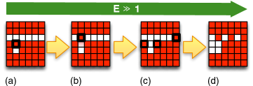
Figure 13: (color online) At high densities and strong fields, longitudinal clusters of holes (empty squares) are easily reduced to transversal structures and basins. (a) The limit case of a single longitudinal strip of vacancies accessed by a mobile particle (bold bordered) is shown; (b) the particle enters the strip, freeing some new mobile particles; (c) the initial particle is pushed rightward by the field; and finally (d) the remaining mobile particles follow an analogous path and a transversal basin of holes is formed.

If we follow the possible movements of the mobile particle and we consider that it cannot move against the field, we see that after a time which depends on the diffusive vertical process the particle is pushed rightward in the sense of the field. Other particles become mobile and they follow an analogous path, so that eventually the holes are concentrated in a basin that has lost the original longitudinal form in favor to a more transversal structure, similar to what was directly inspected in the snapshots of the evolution.

From this brief discussion we see that a general mechanism for the formation of the walls exists and depends actually on the probability of reversal moves $p_{back}$. We also recognize that, at high densities, if we have wide and compact empty regions and adjacent wide and compact filled regions, small “impurities” formed by isolated empty sites play an important role in making specific particles mobile.

VI.2 Exponential distributions

In order to properly justify the choice of the observable associated with the formation of domain walls, we have computed the distribution of the transversal wall sizes: the data have been collected letting a system in its steady state evolve for  20 relaxation times and scanning the whole lattice at each Montecarlo step. Moreover, we repeated the process for 150 samples, in order to smooth the distribution. Clearly, any distribution of lengths extracted from a simulation is affected by finite size effects (i.e. the tails of the distributions are bounded by the system size) so we are interested in large systems. We have chosen, for the majority of the results shown in the following figures, $L=100$, given that the crossover length obtained in ToBiFi for the undriven Kob-Andersen model ranges from $\Xi_{0.8}\approx 16$ to $\Xi_{0.82}\approx 21$ for values of $\rho$ between $0.80$ and $0.82$.

What we get in terms of the distributions is shown in figure 14 for the density $\rho=0.80$. We plot also the occurrence of very small structures of size 1 in order to show that they are at odds with respect to the rest of the data points. Indeed, the picture we get is that the distribution of transversal sizes has an exponential form $P(w)\propto e^{{-w/\langle w\rangle}}$ in a wide region bounded by the very small structures of size 1 and 2 (which are in the limit of the definition of a wall itself) and the tail of very large walls (which are rare and whose observation also depends on the system size). We see that at $E=0$ such a distribution is very clearly an exponential and also interpolates walls of size 1. As the field intensity increases, two behaviors emerge that correspond roughly to the two current regimes: in both regimes, we have a large number of very small structures, but the occurrence of larger walls increases until a final distribution is reached which is almost the same both for $E=2$ (around the current peak) and $E=6$ (far deep in the negative resistance region). Very similar distributions are obtained for different densities, even if the $J(E)$ curves at different $\rho$ have been shown to be quite different (see inset of fig. 2 for comparison): for this reason we have collapsed all the distributions with respect to their average wall size, showing that a common behavior exists for any density (see right panel of fig. 14). The interesting feature of the exponential distribution is that it properly defines a very pertinent observable, the characteristic wall size $\langle w\rangle$ corresponding to the average. The value of the average depends on the region of integration of the distribution: therefore, there is an important dependence of the obtained value on the inferior limit of integration, given that the upper bound corresponds to the size of the simulated system. In our case, we have chosen to ignore only the 1-site-long walls and compute the averages as if the walls were well defined for any size $\geq 2$, obtaining the result in figure 12.

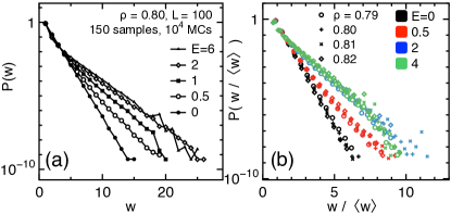
Figure 14: (color online) (a) Distribution of the transversal wall sizes. Excluding the very small structures necessary to the diffusive dynamics, clear exponential tails are established, defining a typical transversal wall length. (b) Distributions of the transversal wall sizes for different values of the external field, rescaled with respect to the average walls size value at densities $0.79,0.80,0.81,0.82$. For each value of the external field, the distributions computed at different densities collapse and at a large field converge to the same distribution.

VI.3 Current and traps

A phenomenological argument that allows for a fit expression of $J(E)$ with respect to $w(E)$ is the following. Let us say that the current flowing into the system has the form

$$J(E,\rho)=A(\rho)(1-{\rm e}^{-E})(1-p_{blocked}(E,\rho))$$ (8)

where $p_{blocked}(E,\rho)$ is simply the probability to pick a blocked configuration. We state that such a probability is expected to be, at a first order of approximation, proportional to the average transversal length of the domain walls. We show this with a concise reasoning: with a coarse grained view of the system, we can say that each domain wall blocks a number of particle which is proportional to its length. If we suppose that the spacing between the different walls $l_{w}$ depends only on the density, and we call $N_{w}$ the total number of walls, we can say that the average number of blocked sites is $n_{blocked}\approx N_{w}\langle w\rangle l_{w}$ and the probability

$$p_{blocked}\approx\frac{N_{w}\langle w\rangle l_{w}}{\rho L^{2}}$$ (9)

where $\rho L^{2}$ is the total number of particles. Assuming that the walls are uniformly distributed, we can estimate $N_{w}\propto\frac{L^{2}}{l^{2}_{w}}$ and finally write that

$$p_{blocked}\approx\alpha(\rho)\langle w\rangle(E,\rho)\propto\frac{\langle w\rangle(E,\rho)}{\rho l_{w}}$$ (10)

where $\alpha(\rho)$ is only a fitting constant. We obtain then an empirical fitting expression

$$J(E,\rho)=A(\rho)(1-e^{-E})[1-\alpha(\rho)\langle w\rangle(E,\rho)]$$ (11)

where both $A$ and $\alpha(\rho)$ should depend on the density of the system and are pure fitting parameters. This naive approach gives good results for densities near the critical value $\rho_{c}=0.79$, as shown in figure 15, but fails for larger densities. It is also harder to reach the steady state at high densities and fields and properly compute the probability distribution of the wall sizes.

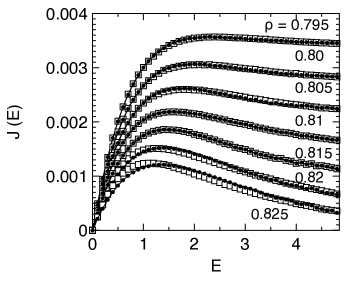
Figure 15: Simulated flow curves (white squares) fitted by the phenomenological model $J(E)=A(1-e^{-E})(1-\alpha\langle w\rangle)$ (black dots). Densities range from $0.795$ to $0.825$, $L=100$, and $\langle w\rangle$ is determined independently from the simulation.

Nevertheless, this approach can explain on a phenomenological basis the crossover region from the flowing to the blocking regime, with a formal expression analogous to what was proposed in JKGC , given that $\langle w\rangle$ is a bounded growing function on the external forcing.

VII Conclusions

We have investigated the spatio-temporal features of a simple kinetically constrained model driven into a non-equilibrium stationary state by a constant and uniform drive. The model can be considered as a generalization of the ASEP with an extra ingredient (the kinetic constraints) schematically representing the cage effect of glassy dynamics. In this type of systems the interplay between kinetic constraints and driving force generates some counterintuitive features which are observed in more complex driven athermal systems, such as highly packed colloidal suspensions and granular materials under shear. Despite the minimalistic rules of our model, we found a rich transport behavior including a crossover from a linear-response regime, at weak field and low density, to a negative resistance regime at strong field and high density, and asymptotically broken ergodicity. We have shown that the flow reduction in the negative resistance regime is related to the emergence of a complex self-organization of dynamical structures which evolve intermittently and exhibit anomalous diffusion. Intermittency is due to the competition between active and inactive regions, so that the system evolves through the alternative succession of low and high mobility configurations, compatibly with the scenario of a dynamical phase transition suggested by the thermodynamics of histories analysis TurciPitard . As observed in other facilitated or kinetically constrained models Jung:2004vo ; JKGC ; Shokef ; Redner , the appearance of dynamical heterogeneities is accompanied by enhanced diffusivity and is closely related to the intermittency in the formation and disruption of particle clusters. A systematic analysis of the typical space and time averaged observables of complex liquids shows that there are several interesting features associated with transport. These include a dynamically induced short-range particle attraction in the transversal direction, which is a signature of an enhanced particle clustering, and a regime of super-diffusion behavior in the longitudinal direction, whose duration increases at a larger applied field. We have highlighted the intermittent and heterogeneous nature of the dynamics by a careful analysis of the trajectories of motion of the particles that actually contribute to the global relaxation, and provided a phenomenological explanation of the crossover to the negative resistance regime. We have determined the characteristic dynamical length of the system and its dependence on the drift, connecting the detailed microscopic configuration space structure to the macroscopic flow. Further investigations concerning the spatial distribution of the correlated walls of holes would improve the understanding of the relationship between the two-folded behavior of the current and the growth of $\langle w\rangle(E)$ with increasing the field strength.

Several future developments can be envisaged. Extensions and generalizations of the present model shall explore other spatio-temporal features of non-equilibrium steady states. First, since the dynamics at strong fields and high densities partitions the systems in mobile and immobile dynamical regions, it would be interesting to analyze how the mobility percolates through the system and what are the geometric properties of the network of mobile particles when a space-dependent driving force (mimicking an applied shear stress) is applied. This would be necessary to address the transition from the shear-thinning to shear-thickening behavior in a more realistic setup. Second, the boundary conditions could be modified by including static walls parallel to the transport direction and different species of particles. That would allow one to explore the effect of confinement and entropic sorting of particles entropicsorting . This could be compared with the case in which the wall is transversal to the applied field (as in granular materials under gravity) where layering phenomena near the wall and segregation effects have been observed SeAr . Third, it would be interesting to extend our approach to the case in which transport is induced by external particle reservoirs Se . Finally, one could modify our model by imposing velocity kinks randomly in space and time to the particles, the dynamics without the kinks obeying the same dynamical constraints as before: this would allow one to investigate the possible emergence of congested traffic motion in active fluids cugliandolo ; wolynes ; vicsek ; active-part-review ; giomi-liverpool-marchetti ; heidenreich .

Acknowledgements - We are grateful to I. Neri for the interpretation of equation (2), and to V. Lecomte, F. van Wijland, J. Kurchan and L. Berthier for interesting discussions. FT is supported by the French Ministry of Research and EP by CNRS and PHC No. 19404QJ.

References

- (1) For reviews see: H. Sillescu, J. Non-Cryst. Solids 243, 81 (1999); M.D. Ediger, Annu. Rev. Phys. Chem. 51, 99 (2000); S.C. Glotzer, J. Non-Cryst. Solids, 274, 342 (2000); R. Richert, J. Phys. Condens. Matter 14, R703 (2002); H. C. Andersen, Proc. Natl. Acad. Sci. U. S. A. 102, 6686 (2005).
- (2) Dynamical heterogeneities in glasses, colloids, and granular media, edited by L. Berthier, G. Biroli, J-P Bouchaud, L. Cipelletti and W. van Saarloos (Oxford University Press, Oxford, 2011).
- (3) R.G. Larson, The Structure and Rheology of Complex Fluids (Oxford University Press, Oxford, 1999).
- (4) Soft and Fragile Matter: Non-equilibrium Dynamics, Metastability and Flow, edited by M.E. Cates and M.R. Evans (IoP, London 2000).
- (5) Jamming and Rheology: Constrained Dynamics on Microscopic and Macroscopic Scales, edited by A. Liu and S.R. Nagel (Taylor & Francis, London 2001).
- (6) F. Ritort and P. Sollich, Adv. Phys. 52, 219 (2003).
- (7) J.P. Garrahan, P. Sollich and C. Toninelli, in Dynamical Heterogeneities in Glasses, Colloids, and Granular Media, edited by L. Berthier, G. Biroli, J.-P. Bouchaud, L. Cipellietti, and W. van Saarloos (Oxford University Press Oxford, 2011), Chap. 10.
- (8) M. Sellitto, Phys. Rev. Lett. 101, 048301 (2008).
- (9) M. Sellitto, Phys. Rev. E 80, 011134 (2009).
- (10) F. Turci and E. Pitard, Europhys. Lett. 94, 10003 (2011)
- (11) J.P. Garrahan, R.L. Jack, V. Lecomte, E. Pitard, K. van Duijvendijk and F. van Wijland , Phys.Rev.Lett. 98, (2007) 195702. J. Phys. A 42, (2009) 075007. E. Pitard, V. Lecomte and F. Van Wijland, Europhys. Lett. 96, 56002 (2011).
- (12) W. Kob and H.C. Andersen, Phys. Rev. E 48, 4364 (1993).
- (13) J. Kurchan, L. Peliti, and M. Sellitto, Europhys. Lett. 39, 365 (1997)
- (14) S. Franz, R. Mulet and G. Parisi, Phys. Rev. E 65, 021506 (2002).
- (15) C. Toninelli, G. Biroli, D.S. Fisher, Phys. Rev. Lett 92, 185504 (2004).
- (16) E. Marinari and E. Pitard, Europhys. Lett. 69, 235 (2005).
- (17) P. Chaudhuri, S. Sastry and W. Kob, Phys. Rev. Lett. 101, 190601 (2008)
- (18) R. Pastore, M. P. Ciamarra, A. de Candia and A. Coniglio, Phys. Rev. Lett. 107, 065703 (2011)
- (19) H. Spohn, J. Phys. A 16 4275 (1983).
- (20) R. L. Jack, D. Kelsey, J.P. Garrahan, D. Chandler, Phys. Rev. E 78, 011506 (2008).
- (21) F. Varnik, L. Bocquet, J. L. Barrat, L. Berthier, Phys. Rev. Lett. 90 , 095702 (2003).
- (22) P. Chaudhuri, L. Berthier, and W. Kob, Phys. Rev. Lett. 99, 060604 (2007).
- (23) D.A. Stariolo and G. Fabricius, J. Chem. Phys. 125, 64505 (2006).
- (24) E.I. Levin, B. I. Shklovskii, Solid State Communications, 67 (3), (1988).
- (25) J.-P. Bouchaud, in Anomalous Transport: Foundations and Applications, edited by R. Klages, G. Radons, and I.M. Solokov, Wiley-VCH (Berlin, 2008).
- (26) C. Monthus, J.-P. Bouchaud, J. Phys. A 29, 3847 (1996).
- (27) D. Dhar, D. Stauffer, Int. J. Mod. Phys. C 9, 349 (1998).
- (28) Y. J. Jung, J.P. Garrahan and D. Chandler Phys. Rev. E.69, 061205 (2004).
- (29) Y. Shokef and A. Liu, Europhys. Lett. 90, 26005 (2010).
- (30) A. Gabel, P.L. Krapivsky and S. Redner, Phys. Rev. Lett. 105, 210603 (2010).
- (31) D. Reguera, A. Luque, P. S. Burada, G. Schmid, J. M. Rubi, and P. Hanggi Phys. Rev. Lett. 108, 020604 (2012).
- (32) M. Sellitto, and J.J. Arenzon, Phys. Rev. E 62, 7793 (2000). Y. Levin, J.J. Arenzon and M. Sellitto, Europhys. Lett. 55, 767 (2001).
- (33) M. Sellitto, Phys. Rev. E 65 020101 (2002).
- (34) D. Loi, S. Mossa, and L. F. Cugliandolo, Physical Review E 77, 051111 (2008).
- (35) A. Czirok and T. Vicsek, Physica A 281, 17 (2000).
- (36) P. Romanczuk, M. Baer, W. Ebeling, B. Lindner, and L. Schimansky-Geier, Eur Phys J-Spec Top 202, 1 (2012).
- (37) S. Wang and P. G. Wolynes, Proc Natl Acad Sci USA 108, 15184 (2011).
- (38) L. Giomi, T. B. Liverpool, and M. C. Marchetti, Phys. Rev. E 81, 051908 (2010).
- (39) S. Heidenreich, S. Hess, and S. H. L. Klapp, Phys. Rev. E 83,011907 (2011).