A $T$-Matrix Calculation for in-Medium Heavy-Quark Gluon Scattering

Abstract

The interactions of charm and bottom quarks in a Quark-Gluon Plasma (QGP) are evaluated using a thermodynamic 2-body $T$-matrix. We specifically focus on heavy-quark (HQ) interactions with thermal gluons with an input potential motivated by lattice-QCD computations of the HQ free energy. The latter is implemented into a field-theoretic ansatz for color-Coulomb and (remnants of) confining interactions. This, in particular, enables to discuss corrections to the potential approach, specifically hard-thermal-loop corrections to the vertices, relativistic corrections deduced from pertinent Feynman diagrams, and a suitable projection on transverse thermal gluons. The resulting potentials are applied to compute scattering amplitudes in different color channels and utilized for a calculation of the corresponding HQ drag coefficient in the QGP. A factor of $\sim$2-3 enhancement over perturbative results is obtained, mainly driven by the resummation in the attractive color-channels.

I Introduction

The description of the Quark-Gluon Plasma (QGP) requires an understanding of how its constituents propagate in the heat bath. The information on pertinent transport properties can ultimately be used to understand how the dense matter produced in heavy-ion colliders such as RHIC and LHC evolves. A starting point of such investigations is the basic two-body interaction between constituents of the QGP. The identification of an in-medium force is a formidable task, especially in a nonperturbative regime as is likely present in the QGP close to the critical temperature, $T_{c}$, and up to 2-3 times its value. For example, lattice-QCD (lQCD) calculations of the heavy-quark (HQ) free energy have found that contributions from the confining force, i.e., linear in the separation, $r$, between heavy quark ($Q$) and anti-quark ($\bar{Q}$), persist up to well above $T_{c}$ Pisarski:2002ji ; Kaczmarek:2005ui ; Petreczky:2004 . The HQ sector is particularly suitable to study the basic QCD two-body force since a large quark mass renders elastic interactions with spacelike exchange kinematics dominant. This leads to a potential interaction which facilitates the reduction of a pertinent scattering equation from the 4-dimensional Bethe-Salpeter one to a 3-dimensional Lippmann-Schwinger PhysRevC.38.51 form. As emphasized in Ref. Rapp:2009my , the spacelike exchange kinematics prevalent in HQ bound states also applies to the scattering of a single heavy quark, thus opening the possibility for a comprehensive treatment of quarkonia and HQ transport in the QGP Riek:2010fk . This has recently been carried out in a thermodynamic $T$-matrix approach where the input potential is resummed in ladder approximation and medium effects are incorporated in both the interaction kernel and the intermediate particle propagation. Thus far, the interactions of heavy quarks in the QGP have mostly been considered with light quarks vanHees:2007me ; Riek:2010fk , which could be done in a fairly straightforward extension of quarkonia Cabrera:2006wh ; PhysRevC.72.064905 .

In the present work we extend the $T$-matrix approach to HQ-gluon scattering. Compared to the heavy-light quark case, this requires to revisit the relativistic corrections to the potential vertices and associated subtleties due to the different dimension of the scattering amplitude, as well as the appropriate transverse polarization of the in- and outgoing thermal gluons. Once suitable amendments are deduced and implemented we compute the pertinent $T$-matrices in all available color projections and obtain thermal relaxation rates as defined by an underlying Fokker-Planck equation. In particular, we will compare our results to perturbative evaluations in order to quantify the relevance of the confining and higher-order terms in the $T$-matrix.

Our article is organized as follows. In Sec. II we briefly recall the field-theoretical model used to implement the lQCD-motivated static potentials. In Sec. III we discuss the relativistic corrections to the color-Coulomb and confining terms of the potential, with special care of the different dimension of the quark-gluon relative to the quark-quark $T$-matrix and a restriction to transverse degrees of the physical gluons. In Sec. IV we calculate the HQ-gluon $T$-matrices in different color channels and elucidate the role of the confining and the higher-order rescattering terms. In Sec. V we utilize the HQ-gluon $T$-matrices to evaluate the HQ friction coefficient at different temperatures as a function of 3-momentum, decomposed into its color and angular-momentum contributions. We summarize and conclude in Sec. VI.

II Construction of the in-Medium Potential

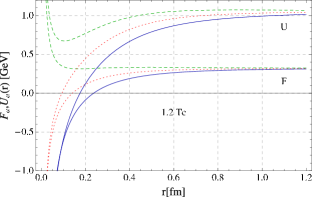
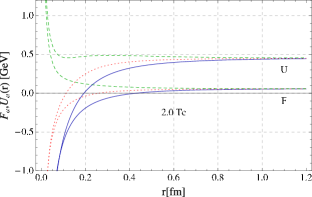
Figure 1: In-medium HQ free and internal energies in the triplet (solid lines), sextet (dotted lines), and 15-plet (dashed lines) channels at temperatures $T=1.2\,T_{c}$ (left) and 2 $T_{c}$ (right). (Color online.)

Recent computations of the static HQ free energy in thermal lQCD Bazavov:2009us have revived potential-based approaches to quarkonia in the QGP. Since a functional fit to static coordinate-space quantities is somewhat limited in flexibility for microscopic applications, we follow Ref. Riek:2010fk where a microscopic model Megias:2007pq ; Megias:2005ve for color-Coulomb and confining terms has been adopted. A fit has been performed to the color-average free energies at different temperatures (from 1.2 $T_{c}$ to $\sim$2 $T_{c}$) using 4 model parameters characterizing the overall strength ($\alpha_{s}$, $m_{G}$) and screening properties ($m_{D}$, $\tilde{m}_{D}$) of each of the two contributions (here, we focus on the lQCD data of Ref. Kaczmarek:2007pb , denoted as “potential-1” in Ref. Riek:2010fk ; another set of lQCD data studied therein leads to slightly stronger effects). The different color projections are then obtained as

$$F_{a}(T,r) = -\frac{4}{3}\alpha_{s}(\frac{C_{a}}{r}e^{-m_{D}r}+\frac{m_{G}^{2}}{2\tilde{m}_{D}}e^{-\tilde{m}_{D}r}$$ (1)

$$-\frac{m_{G}^{2}}{2\tilde{m}_{D}}+m_{D})\ ,$$

where it is assumed that the string interaction (second term), as well as the long-distance limit represented by the last two terms, are color-blind. For the color-Coulomb interaction (first term), one assumes the standard (perturbative) Casimir scaling resulting in the following coefficients for quark-antiquark, quark-quark and quark-gluon channels, respectively PhysRevD.70.054507 ,

$$C_{1} = 1\qquad,\ C_{8}=-1/8\ ,$$

$$C_{6} = -1/4\ ,\ C_{\bar{3}}=1/2\ \ \ ,$$

$$C_{3} = 9/8\quad\,,\ C_{6}=3/8\ \ \ ,\ C_{15}=-3/8\ .$$ (2)

The internal energy follows as

$$U(T,r)=F(T,r)-T\frac{d}{dT}F(T,r)\ .$$ (3)

The resulting coordinate-space potentials in the HQ-gluon color projections are summarized in Fig. 1.

There is currently no consensus as to whether the free or internal energy (or combinations thereof) should be used as a static potential in a Schrödinger (or Lippmann-Schwinger) equation. We will perform our calculations for both $U$ and $F$. As usual, we will subtract off the infinite-distance limit to define the genuine two-body interaction contribution in each case,

$$V_{a}(T,r)=X_{a}(T,r)-X(T,\infty)\hskip 4.33601pt,\hskip 4.33601ptX=F\text{ or }U\ ,$$ (4)

and reinsert $X(T,\infty)$ into the calculation by interpreting it as a temperature-dependent mass term of the heavy anti-/quarks. For a more reliable application at higher energies, it remains to elaborate the effects of relativistic corrections for the case at hand, i.e., HQ-gluon scattering.

III Relativistic Corrections to Potential Terms

Diagrams/tchannelgluon (45,30) i1,i2 o1,o2

$p_{1}$i1 $p_{2}$i2 $p_{3}$o1 $p_{4}$o2

fermioni1,v1,o1 curlyi2,v2,o2 curlyv1,v2

Figure 2: Feynman diagram for $Q$-$g$ scattering via $t$-channel gluon exchange. In the center-of-mass system, $q=(p_{2}-p_{1})/2$ and $q^{\prime}=(p_{4}-p_{3})/2$.

To identify relativistic corrections to the nonrelativistic potential we will be analyzing Feynman diagrams associated with the Coulomb and string terms, $V_{c}$ and $V_{s}$, respectively. For the Coulombic part, we refer to the $t$-channel exchange diagram for quark-gluon scattering displayed in Fig. 2 (Compton scattering diagrams with an intermediate HQ propagator are parametrically suppressed by a power of the HQ mass). To establish a relationship between the fully relativistic scattering amplitude, $\mathcal{M}$, and the nonrelativistic $T$-matrix, $T$ (following from the Fourier transform of the static coordinate-space potential), we write down pertinent expressions of the cross section. For fermion-boson scattering with Bjorken-Drell conventions (where the Dirac spinors are normalized as $\bar{u}u=1$), the former reads bjorken1964relativistic

$$d\sigma = \frac{(2\pi)^{4}m_{1}m_{3}}{\omega_{1}\omega_{2}|\mathbb{v}_{1}-\mathbb{v}_{2}|}\int\frac{d^{3}p_{3}}{2\omega_{3}(2\pi)^{3}}\frac{d^{3}p_{4}}{2\omega_{4}(2\pi)^{3}}$$ (5)

$$\times|\mathcal{M}|^{2}\delta^{(4)}(p_{3}+p_{4}-p_{1}-p_{2})\ ;$$

note that in this convention $\mathcal{M}$ carries the dimension of inverse energy, dim$(\mathcal{M})=E^{-1}$ (for fermion-fermion scattering, dim$(\mathcal{M})=E^{-2}$, see also Ref. Riek:2010fk ; this is convenient for taking the nonrelativistic limit to recover the nonrelativistic $T$-matrix). In terms of the nonrelativistic $T$-matrix, the cross section can be expressed as goldberger2004collision

$$d\sigma = \frac{(2\pi)^{4}}{\omega_{1}\omega_{2}|\mathbb{v}_{1}-\mathbb{v}_{2}|}\int\frac{d^{3}p_{3}}{2\omega_{3}(2\pi)^{3}}\frac{d^{3}p_{4}}{2\omega_{4}(2\pi)^{3}}$$

$$\times|\sqrt{\omega_{1}\omega_{2}}T\sqrt{2\omega_{3}2\omega_{4}}|^{2}\delta^{(4)}(p_{3}+p_{4}-p_{1}-p_{2})\ .$$

Comparison with Eq. (5) thus leads to

$$\sqrt{\omega_{1}\omega_{2}}T\sqrt{2\omega_{3}2\omega_{4}}=\sqrt{m_{1}m_{3}}\mathcal{M}\ .$$ (7)

In Ref. Herrmann:1992 the relation between the nonrelativistic $T$-matrix and a properly generalized relativistic form, $\tilde{T}$, has been worked out for the fermion-fermion case as

$$T=\sqrt{\frac{m_{1}m_{2}m_{3}m_{4}}{\omega_{1}\omega_{2}\omega_{3}\omega_{4}}}\tilde{T}\ ,$$ (8)

which is the same result obtained in Ref. Riek:2010fk , i.e., $\tilde{T}$ is the relevant quantity for our purposes here. However, since we are interested in fermion-boson scattering, an additional dimensionful normalization factor appears. This can be obtained by inserting the expression for $\tilde{T}$ from Eq. (8) into Eq. (7). One obtains

$$\tilde{T}=\frac{1}{\sqrt{2m_{2}2m_{4}}}\mathcal{M}\ ,$$ (9)

where we recall that $\mathcal{M}$ is the fully relativistic scattering amplitude in Bjorken-Drell normalization.

To proceed, we consider the Born approximation, where $\tilde{T}=\tilde{V}$, and evaluate $\mathcal{M}$ using Feynman diagrams from an underlying Lagrangian. As before, we split $\mathcal{M}$ into a Coulombic and string part,

$$\mathcal{M}=\mathcal{M}_{c}+\mathcal{M}_{s}\ ,$$ (10)

where the Coulombic part is given by the gluon-exchange diagram in Fig. 2 and the string contribution by Fig. 4. Let us first consider the Coulomb part which we factorize into a Yukawa-like propagator including coupling and color factors and a spinor-dependent quantity,

$$\mathcal{M}_{c}=-i \underbrace{\frac{C_{A}g^{2}}{t-m_{D}^{2}}}\underbrace{\bar{u}(p_{3})(-i\gamma^{\mu})u(p_{1})\epsilon(p_{4})_{\rho}^{*}\Gamma^{\rho\lambda}_{\mu}\epsilon(p_{2})_{\lambda}}\ ,$$

YukawaSpinor (11)

where $u$ denote the HQ spinors, $\epsilon^{\mu}$ the gluon polarization vectors, $\Gamma^{\rho\lambda}_{\mu}$ the 3-gluon vertex, and $1/({t-m_{D}^{2}})$ the gluon-exchange propagator. The 3-gluon vertex is given by

$$\Gamma^{\rho\lambda}_{\mu}= -(-g^{\rho\lambda}(p_{4}+p_{2})_{\mu}+g^{\lambda}_{\mu}(p_{2}-q)^{\rho}$$

$$+g^{\rho}_{\mu}(q+p_{4})^{\lambda})\ .$$ (12)

The Yukawa part is merely the Fourier transform of the Coulombic static potential ansatz given in Eq. (4), while the second factor encodes the relativistic corrections. That is,

$$\tilde{V}_{c}=\frac{V_{c}}{\sqrt{2m_{2}2m_{4}}}|-i\bar{u}(p_{3})(-i\gamma^{\mu})u(p_{1})\epsilon(p_{4})_{\rho}^{*}\Gamma^{\rho\lambda}_{\mu}\epsilon(p_{2})_{\lambda}|\ .$$ (13)

The spinor part is calculated by taking its square and then contracting across the vertices. This allows to read off the leading relativistic corrections to our static potential ansatz (a similar procedure will be carried out for the string term, cf. Eq. (40) and below).

A consistent treatment at finite temperature requires the consideration of thermal vertex corrections which we analyze within the Hard Thermal Loop (HTL) framework. For the 3-gluon vertex, we have contributions from a gluon loop, ghost loop and quark loop as illustrated in Fig. 3.

Diagrams/gluonloop (0,0)(0,7) .4 (45,30) i1 o1,o2 $p_{1}$i1 $p_{3}$o1 $p_{2}$o2 curly,tension=3,width=.01i1,v1 curly,tension=1v1,v3 curly,tension=1v1,v2 curly,tension=.1v3,v2 curly,tension=3v2,o2 curly,tension=3v3,o1 Diagrams/ghostloop (0,0)(0,7) .4 (45,30) i1 o1,o2 $p_{1}$i1 $p_{3}$o1 $p_{2}$o2 curly,tension=3,width=.01i1,v1 dashes,tension=1v1,v3 dashes,tension=1v1,v2 curly,tension=.1v3,v2 curly,tension=3v2,o2 curly,tension=3v3,o1

Diagrams/quarkloop (0,0)(0,7) .4 (45,30) i1 o1,o2 $p_{1}$i1 $p_{3}$o1 $p_{2}$o2 curly,tension=3,width=.01i1,v1 plain,tension=1v1,v3 plain,tension=1v1,v2 plain,tension=.1v3,v2 curly,tension=3v2,o2 curly,tension=3v3,o1

Diagrams/gluoncircleloop

.4 (45,30) i1 o1 b1,b2,b3 t1 $p_{1}$b1 $p_{2}$t1 $p_{3}$b3 curlyb1,b2,b3 curly,left=1,tension=.3b2,v2,b2 curlyv2,t1

Figure 3: Contributions to the 3-gluon vertex corrections. Curly, solid and dashed lines represent gluons, quarks and ghosts, respectively.

The gluon contribution reads

$$\Gamma^{(gl)}(p_{1},p_{2},p_{3})= ig^{3}C_{A}f_{abc}\int\frac{d^{4}k}{4\pi}9{k}_{\mu}{k}_{\nu}{k}_{\rho}$$

$$\times\Delta(k)\Delta(p_{2}-k)\Delta(p_{3}+k)\ ,$$ (14)

where the $\Delta$’s indicate intermediate gluon propagators. Utilizing standard power counting techniques Braaten:1990 ; Braaten1990310 , the propagator contributions will schematically integrate to

$$\int\frac{d^{4}k}{(2\pi)^{4}}\Delta(k)\Delta(p_{2}-k)\Delta(p_{3}+k)\propto\int\frac{dk}{kp}X\ ,$$ (15)

where $X$ depends on the quantum statistics of the interacting particles. There are three possible cases: (i) $X$ involves a sum of statistical factors of the same kind (both fermion or both boson), (ii) $X$ is a difference of statistical factors of the same kind, and (iii) $X$ is a difference of statistical factors of different kinds. Case (i) and (ii) occur for the 3-gluon vertex, while (iii) occurs for the quark-gluon vertex. However, case (i) will drop out because it is associated with a $T=0$ divergence, and the 3-gluon vertex is only linearly divergent. Examining the 3-gluon vertex (ii), we have, schematically, $X\propto\frac{dn}{dk}\rightarrow 1/T$. Combining the above equation with the kinematic contributions of the vertex, the gluon HTL correction will behave as

$$g^{3}\int\frac{dk}{kp}k^{3}X\propto g^{3}T^{2}p^{-1}\ .$$ (16)

Thus, for $p\sim gT$ the HTL correction is of order $g^{2}T$, which is the same as the zeroth order 3-gluon vertex. However, in the regime of interest here, the gluons in the heat bath are hard and thus $p\approx T$. This renders HTLs subleading and it is sufficient to use the bare vertex at finite temperature. A similar argument is carried out for the quark-gluon vertex and the other loop corrections displayed in Fig. 3.

Let us now return to the task of analyzing the diagrammatic representation of our potential. Toward this end we calculate the potential $\tilde{V}_{c}$ by utilizing completeness relations that sum over spin ($s$) and polarization states ($r$),

$$\sum_{s}u_{\mu}(p,s)\bar{u}_{\nu}(p,s)=\Big{(}\frac{\not{p}+m}{2m}\Big{)}_{\mu\nu}\ ,$$ (17)

$$\sum_{r}\epsilon^{*}_{\mu}(p,r)\epsilon_{\nu}(p,r)=g_{\mu\nu}-\frac{p_{\mu}p_{\nu}}{m^{2}}\ .$$ (18)

The spinor terms in Eq. (11) are evaluated by first replacing the $u$’s with the completeness relation from Eqs. (17,18),

$$\Pi=|\bar{u}(p_{3})\gamma {}^{\mu}u(p_{1})\epsilon(p_{4})_{\rho}^{*}\Gamma^{\rho\lambda}_{\mu}\epsilon(p_{2})_{\lambda}|^{2}$$

$$= \frac{\text{Tr}\{(\not{p_{3}}+m_{1})\gamma^{\mu}(\not{p_{1}}+m_{1})\gamma^{\sigma}\}}{4m_{1}^{2}}$$ (19)

$$\times\Gamma^{\rho\lambda}_{\mu}\Gamma^{\alpha\beta}_{\sigma}E_{\alpha\beta}E_{\rho\lambda}\ ,$$

where the $\Gamma$ and $E$ tensors are defined as

$$\Gamma^{\rho\lambda}_{\mu}= -(-g^{\rho\lambda}(p_{4}+p_{2})_{\mu}+g^{\lambda}_{\mu}(p_{2}-q)^{\rho}$$

$$+g^{\rho}_{\mu}(q+p_{4})^{\lambda})\ ,$$ (20)

$$E_{\mu\nu}= g_{\mu\nu}-\frac{p_{\mu}p_{\nu}}{m_{2}^{2}}\ .$$ (21)

Contracting across the $\Gamma$’s and a term being traced over with computational tools Mertig1991345 , we utilize standard Mandelstam variables to simplify the result,

$$s= (p_{1}+p_{2})^{2}\rightarrow p_{1}\cdot p_{2}=\frac{1}{2}(s-p_{1}^{2}-p_{2}^{2})\ ,$$ (22)

$$t= (p_{1}-p_{3})^{2}\rightarrow p_{1}\cdot p_{3}=-\frac{1}{2}(t-p_{1}^{2}-p_{3}^{2})\ ,$$ (23)

$$u= (p_{1}-p_{4})^{2}\rightarrow p_{1}\cdot p_{4}=\frac{1}{2}(-s-t$$

$$+m_{1}^{2}+m_{2}^{2}+m_{3}^{2}+m_{4}^{2}-p_{1}^{2}-p_{4}^{2})\ ,$$ (24)

where for the last line we have used $s+t+u=m_{1}^{2}+m_{2}^{2}+m_{3}^{2}+m_{4}^{2}$. Furthermore, we employ the on-shell conditions $p^{2}=m^{2}$ for in- and outgoing particles. Following Ref. Riek:2010fk , we drop terms of order $t$ or higher relative to $s$, $m_{Q}^{2}$. This is justified in the high-energy elastic limit which is the one of interest to infer the relativistic corrections. We now have an expression with $\sim$200 terms that must be contracted with the remaining vector-boson completeness relation. An important feature for the thermal gluon is that it should not exhibit the 3 degrees of freedom expected from a massive spin-1 vector-boson, since the longitudinal degree of freedom is not observed in the high-temperature limit of the QGP equation of state computed in lQCD PhysRevC.57.1879 ; Cheng:2007jq . To enforce this characteristic, we project out the transverse modes with the help of the usual projection operators,

$$(P_{T}+P_{L})_{\mu\nu}=g_{\mu\nu}-\frac{p_{\nu}p_{\mu}}{m^{2}}\ ,$$ (25)

$$(P_{T})_{ij}=\delta_{ij}-\frac{p_{i}p_{j}}{m^{2}}\ ,$$ (26)

$$(P_{T})_{00}=(P_{T})_{0i}=(P_{T})_{j0}=0\ ,$$ (27)

where $i=1,2,3$. By selecting $P_{T}$, we proceed with the contraction that schematically is viewed as

$$\Pi_{T}=\Lambda^{ijkl}(P_{T})_{ij}(P_{T})_{kl}=\Lambda^{ijkl}E_{ij}E_{kl}\ ,$$ (28)

with $\Lambda$ representing the result of the first contraction. We are then left with a series of purely 3-D scalar products. To see this, we rework the Mandelstam relations for 3-momenta,

$$\mathbf{p}_{1}\cdot\mathbf{p}_{2}=\frac{1}{2}(-s+m_{1}^{2}+m_{2}^{2}+2\omega_{1}\omega_{2})\ ,$$ (29)

$$\mathbf{p}_{1}\cdot\mathbf{p}_{3}=-\frac{1}{2}(t-m_{1}^{2}-m_{3}^{2}+2\omega_{1}\omega_{3})\ ,$$ (30)

$$\mathbf{p}_{1}\cdot\mathbf{p}_{4}=\frac{1}{2}(-s-t+m_{2}^{2}+m_{3}^{2}+2\omega_{1}\omega_{4})\ ,$$ (31)

where $E_{i}=\omega_{i}=\sqrt{m_{i}^{2}+\mathbf{k}_{i}^{2}}$. In the center of mass (CM) of an elastic collision, we set $\omega_{1/2}=\omega_{3/4}$ and $\mathbf{p}_{1/3}=-\mathbf{p}_{2/4}$. Thus,

$$\Pi_{T}=$$

$$\frac{2}{m_{1}^{2}}\Big{(}(-{\mathbf{p}_{1}}^{2}({m_{1}}^{2}-{\omega_{1}}^{2})({m_{2}}^{2}+{m_{1}}^{2}-s+2{\omega_{1}}{\omega_{2}})^{2}$$

$$+({m_{2}}^{2}-{\omega_{2}}^{2})^{2}({m_{2}}^{2}+{m_{1}}^{2}-s)^{2}+2{\mathbf{p}_{1}}^{8})\frac{1}{{\mathbf{p}_{1}}^{4}}$$

$$-4{\omega_{1}}{\omega_{2}}({m_{2}}^{2}+{m_{1}}^{2}-s)-2({m_{1}}^{2}-{\omega_{1}}^{2})^{2}-4{\omega_{1}}^{2}{\omega_{2}}^{2}\Big{)}\ ,$$ (32)

which, upon averaging over spin states, can be further simplified to

$$\Pi_{T}=\frac{1}{m_{1}^{2}}(s-m_{2}^{2}-m_{1}^{2})^{2}\ .$$ (33)

We take $\Pi_{T}$ as the result of the spinor structure calculation and ignore the longitudinal mode. We set $m_{2/4}=m_{g}$ and $m_{1/3}=m_{Q}$. Referring back to Eq. (13), our modified potential, $\tilde{V}_{c}$, thus reads

$$\tilde{V}_{c}=V_{c}\sqrt{\frac{(s-m_{g}^{2}-m_{Q}^{2})^{2}}{4m_{g}^{2}m_{Q}^{2}}}\ .$$ (34)

We see that $\Pi_{T}/4m_{g}^{2}$ yields the same corrections as found for the heavy-light quark case elaborated in Ref. Riek:2010fk ; we adopt the notation in there to summarize our relativistic corrections as

$$R(q,q^{\prime})= m(q)^{-1/2}m(q^{\prime})^{-1/2}\ ,$$ (35)

$$B(q,q^{\prime})= b(q)^{1/2}b(q^{\prime})^{1/2}\ ,$$ (36)

$$b(q)= (1+\frac{q^{2}}{\omega_{g}(q)\omega_{Q}(q)})\ ,$$ (37)

$$m(q)= \frac{m_{Q}m_{g}}{\omega_{Q}(q)\omega_{g}(q)}\ .$$ (38)

The relativistically augmented Coulomb potential for HQ-gluon scattering then reads

$$\tilde{V}_{c}=V_{c}\ R(q,q^{\prime})\ B(q,q^{\prime})\ .$$ (39)

We now perform the same analysis on the string portion of the potential which requires an ansatz for a pertinent Lagrangian. Assuming the string interaction to be of scalar type one has

$$\mathcal{L}=\tilde{G}m_{g}A^{\mu}A_{\mu}\bar{Q}Q\ ,$$ (40)

which is characterized by a dimensionful coupling, $\tilde{G}$, which in momentum space recovers the Fourier transform of the static linear coordinate-space potential, $V_{s}\sim m_{G}^{2}/(\mathbf{k}^{2}+\tilde{m}_{D}^{2})^{2}$. As in the Coulomb case, we can then write down the amplitude (in Bjorken-Drell normalization) as a potential with relativistic corrections from the spinor terms,

$$\tilde{V}_{s}=\frac{V_{s}}{2m_{g}}|\bar{u}(p_{3})u(p_{1})2m_{g}\epsilon(p_{4})_{\mu}^{*}\epsilon(p_{2})^{\mu}|\ .$$ (41)

Diagrams/scalar (45,30) i1,i2 o1,o2 $p_{1}$i1 $p_{2}$i2 $p_{3}$o1 $p_{4}$o2 fermioni1,v1,o1 curlyi2,v1,o2

Figure 4: Schematic approximation of the nonperturbative string term by a scalar 4-point interaction.

Calculating the spinor terms with transverse gluons yields

$$\Xi= |\bar{u}(p_{3})u(p_{1})2m_{g}g^{\mu\nu}\epsilon(p_{4})_{\mu}^{*}\epsilon(p_{2})_{\nu}|^{2}$$

$$\Xi_{T}= \text{Tr}\{(\not{p_{1}}+m_{1})(\not{p_{3}}+m_{3})\}E_{ij}E^{ij}\frac{4m_{g}^{2}}{4m_{Q}^{2}}$$

$$= (8m_{Q}^{2}-2t)(1+\frac{(\mathbb{p}_{2}\cdot\mathbb{p}_{4})^{2}}{\mathbb{p}_{2}^{2}\mathbb{p}_{4}^{2}})\frac{4m_{g}^{2}}{4m_{Q}^{2}}\ .$$ (42)

We can simplify Eq. (23) by plugging our elastic condition, $t=-(\mathbf{p}_{2}-\mathbf{p}_{4})^{2}$, into Eq. (42),

$$\Xi_{T}=8m_{g}^{2}(1+\frac{1}{4}(\mathbb{p}_{2}^{4}+\mathbb{p}_{4}^{4}+2\mathbb{p}_{2}^{2}\mathbb{p}_{4}^{2})(\mathbb{p}_{2}^{2}\mathbb{p}_{4}^{2})^{-1})\ .$$ (43)

Utilizing CM kinematics, $\mathbb{p}_{2}^{2}=\mathbb{p}_{4}^{2}$, Eq. (43) reduces to $\Xi_{T}=16m_{g}^{2}$. Averaging over spin states and dividing through by the normalization factor, one obtains

$$\tilde{V}_{s}=V_{s}\frac{\sqrt{\Xi_{T}/4}}{2m_{g}}=V_{s}\ .$$ (44)

The net result is that the string potential does not develop a relativistic correction within our approximation scheme (again, paralleling the heavy-light quark case Riek:2010fk ).

The parameterization of the static lQCD coordinate potential in principle includes the effect of a running coupling constant at short distances. However, its off-shell extension in the Fourier transform does not, i.e., if the in- and outgoing moduli of the relative 3-momenta are different. We therefore introduce a correction to simulate the off-shell running of $\alpha_{s}$ through a factor

$$\text{F}_{\rm run}(q,q^{\prime})=\text{ln}[\frac{\Delta^{2}}{\Lambda^{2}}]/\text{ln}[\frac{(q-q^{\prime})^{2}+\Delta^{2}}{\Lambda^{2}}]\ ,$$ (45)

with $\Delta=1$ GeV and $\Lambda=0.2$ GeV.

We are now in position to quote the final form our relativistically generalized static potential as

$$\tilde{V}(q,q^{\prime})=R(q,q^{\prime})B(q,q^{\prime})F_{\rm run}(q,q^{\prime})V_{c}(q,q^{\prime})+V_{s}(q,q^{\prime})\ .$$ (46)

Its explicit decomposition into color projections and partial waves reads

$$\tilde{V}^{l,a}(q,q^{\prime})=R(q,q^{\prime})B(q,q^{\prime})F_{\text{run}}(q,q^{\prime})V_{c}^{l,a}(q,q^{\prime})$$

$$+V_{s}^{l}(q,q^{\prime})\ ,$$ (47)

where $l=0,1,2...$ denotes the angular-momentum quantum number and $a$ the color index of the irreducible representations of the triplet-octet system (the Coulomb part follows Casimir scaling while the string term is assumed to be color-blind). As in previous work we neglect spin-orbit and and spin-spin contributions to the potential. Equation (47) is the explicit expression to be used in the pertinent $T$-matrix equations for each combination of $\{l,a\}$.

IV $T$-Matrix

We solve for the $\tilde{T}$-matrix utilizing a 3-D reduced Bethe-Salpeter PhysRev.84.1232 equation in ladder approximation Machleidt:1989tm ; Thompson:1970wt . After partial-wave expansion and color projection we obtain a 1-D integral equation which yields itself to numerical analysis,

$$\tilde{T}^{l,a}(E;q^{\prime},q)=\tilde{V}^{l,a}(q^{\prime},q)+\frac{2}{\pi}\int\limits_{0}^{\infty}dkk^{2}\tilde{V}^{l,a}(q^{\prime},k)$$

$$\times G_{12}(E;k)\tilde{T}^{l,a}(E;k,q)[1-n_{1}(\omega_{1}(k))+n_{2}(\omega_{2}(k))]\ .$$ (48)

The thermal distribution functions, $n_{i}$, figure according to their quantum statistics, i.e., fermion for $i$=1 (heavy quark) and boson for $i$=2 (gluon). At the relevant QGP temperatures of up to 2-3 $T_{c}$ their impact is small (negligible for heavy quarks). As before, $q=|\mathbf{q}|$ and $q^{\prime}=|\mathbf{q}^{\prime}|$ denote the relative 3-momenta of the incoming and outgoing states, respectively, and $k=|\mathbf{k}|$ is the relative (integration-) momentum of the intermediate states. To complete the analysis of our $\tilde{T}$-matrix, we must select a propagator which amounts to specifying the reduction scheme of the underlying 4-D scattering equation. For the present paper we employ the Thompson Thompson:1970wt scheme,

$$G_{gQ}(q)= \frac{m(q)}{E-\omega_{g}(q)-\omega_{Q}(q)-\Sigma_{g}-\Sigma_{Q}}\ ,$$ (49)

where $\omega_{g,Q}(q)=\sqrt{q^{2}+m_{g,Q}^{2}}$, and $m(q)$ is defined in Eq. (38). We motivate the choice of the Thompson scheme by stating that it has been previously suggested Woloshyn:1973 to provide the closest resemblance to the original Bethe-Salpeter equation. As in Ref. Riek:2010fk the masses of the heavy quarks are determined by the sum of a bare mass, $m_{Q}^{0}$, and an in-medium contribution defined by the infinite-distance limit of the potential (free or internal energy),

$$m_{Q}=m_{Q}^{0}+\Sigma_{Q}^{R}(T)\hskip 4.33601pt,\hskip 4.33601pt\Sigma_{Q}^{R}(T)=X(T,\infty)/2\ ,$$ (50)

with $X=F\text{ or }U$. The bare mass is adjusted to the ground-state quarkonium mass in vacuum (where the self-energy contribution, $\Sigma_{Q}^{R}(T=0)$, is evaluated at a typical string-breaking scale of $r\simeq$1-1.2 fm). When using the lQCD potential of Ref. Kaczmarek:2007pb within the Thompson scheme one finds $m_{c}^{0}=1.264$ GeV and $m_{b}^{0}=4.662$ GeV. The in-medium gluon mass, $m_{g}$, is approximated by its expression from thermal perturbation theory bellac2000thermal ,

$$m_{g}^{2}=\frac{g^{2}T^{2}}{2}(\frac{N_{c}}{3}+\frac{N_{f}}{6})\ .$$ (51)

We choose 3 active light flavors ($N_{f}=3$), and with three colors, $N_{c}=3$, the thermal mass correction is $m_{g}=\sqrt{{3}/{4}}gT$. We fix $g=2.3$, which is consistent with lQCD calculations as outlined in Ref. Riek:2010fk ; Cheng:2010 . In the QGP, both heavy quarks and light partons are expected to acquire a substantial width. For charm quarks, it has been computed selfconsistently in Ref. Riek:2010py . For simplicity, we fix the combined width of heavy quark and gluon at $0.2$ GeV, i.e., $0.1$ GeV for each particle. This approximation has been shown previously to give good agreement with the selfconsistent results when computing the HQ relaxation rates, which is our main focus here.

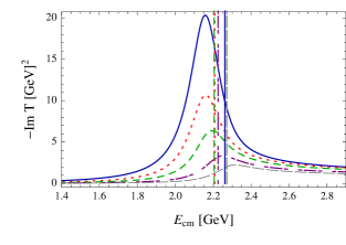
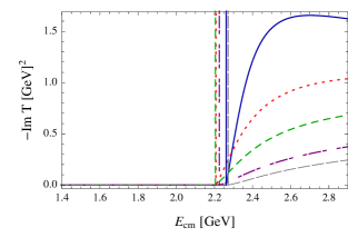
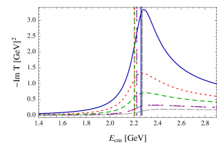
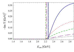
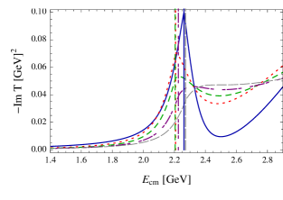
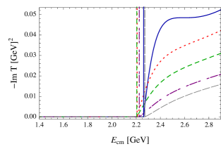
Figure 5: Imaginary part of the on-shell charm-gluon $\tilde{T}$-matrix for $S$-wave (left) and $P$-wave (right) scattering in the triplet (upper), sextet (middle), and 15-plet (bottom) channels using $U$ as a potential and a fixed two-particle width of 200 MeV. Vertical lines indicate the mass threshold at the associated temperature. (Color online.)

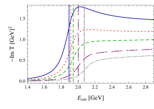
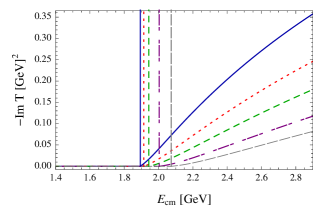
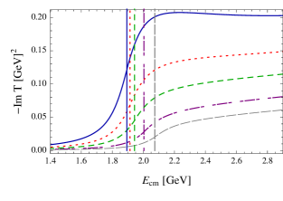
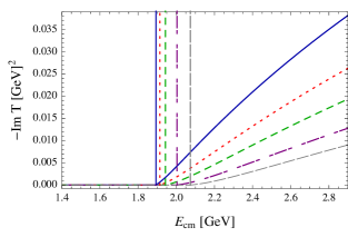
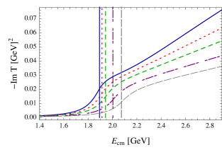
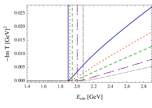
Figure 6: Same as Fig. 5, but using potential $F$.

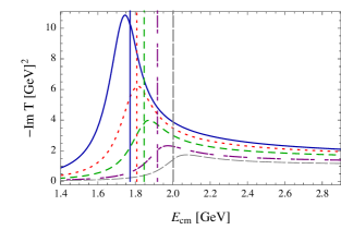
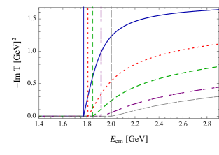
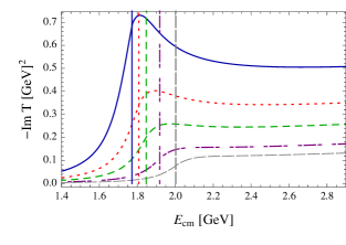
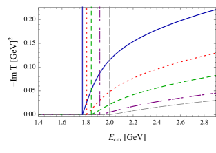
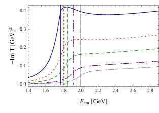
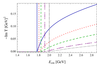
Figure 7: Same as Fig. 5, but for a potential with only the Coulomb term.

The resulting $\tilde{T}$-matrices, depicted in Fig. 5, indicate near-threshold resonances in the attractive triplet and sextet channels up to temperatures of $\sim$1.5 $T_{c}$. The repulsive 15-plet channel is suppressed in strength by more than an order of magnitude in the near-threshold regime, and turns out to be comparable in $S$- and $P$-waves. On the other hand, in the attractive color channels the $P$-waves are substantially suppressed relative to the $S$-waves not too far above threshold, but become comparable well above threshold once the $S$-wave resonance structure ceases. When changing the input potential to the free energy, $F$, (cf. Fig. 6), the 2-particle threshold energy is significantly reduced at low temperatures. Due to the reduced interaction strength, the attractive resonance structures universally disappear in all channels for all temperatures (excluding perhaps the triplet at $1.2T_{c}$); the remaining enhancements in the $S$-waves now mostly occur above the threshold energies. The latter continually increase with temperature, as opposed to the non-monotonic behavior for the internal energy. This is attributed to the dominance of the increasing thermal-mass contribution of the gluon over the weakly decreasing infinite-distance limit of the free energy governing the in-medium HQ mass.

To investigate the relative importance and interplay of the Coulomb and string parts in our potential ansatz, we perform identical calculations for the Coulomb portion only by setting $m_{G}=0$. This, in particular, implies that the infinite-distance limit of the potential is largely reduced, leading to a smaller mass correction (which can even become negative as expected from thermal perturbation theory at high $T$). The smaller mass enhances the potential through the relativistic correction factors in Eq. (35) entailing an increase in the $\tilde{T}$-matrix. On the other hand, the attractive channels experience a loss of attraction due to the missing string term, while in the repulsive channel the compensation effect with the attractive string term is lifted. These effects are quantitatively borne out of Fig. 7. The Coulomb-only $\tilde{T}$-matrices are reduced by up to a factor of 2 (4) in the triplet (sextet) channels in the resonance region, and less so at higher energies and with increasing $T$. On the other hand, the 15-plet increases by a factor of up to $\sim$4 close to threshold and close to $T_{c}$. The sextet and 15-plet thus exhibit the strongest sensitivity since here Coulomb and string term are comparable and thus their interplay is most pronounced (enhancement and compensation, respectively). Another important component is the threshold energy: in the full potential at 1.2 $T_{c}$ the charm-quark mass is $\sim$1.8 GeV, while for Coulomb only it is $\sim$1.3 GeV. This increases the phase space allowing for more possible interactions when the particle propagates in the medium which has important consequences for the HQ transport coefficient. Additionally, in the attractive channels, the Coulomb $\tilde{T}$-matrix peaks somewhat closer to threshold (due to slightly less binding), thus making available more interaction strength in the scattering regime (continuum). In the $P$-wave, the differences in magnitude of the $\tilde{T}$-matrix between the full and Coulomb-only calculations are less pronounced in the attractive channels (higher momenta are probed where the string term is suppressed), while the 15-plet still shows a noticeable enhancement. These dynamic and kinematic effects will be important in the interpretation of the pertinent results for the transport coefficient discussed below.

V Transport Coefficient

To examine the diffusion properties of a single heavy (anti-) quark in the context of our heavy-light $\tilde{T}$-matrix, we adopt the usual Fokker-Planck approach PhysRevD.37.2484 . The relaxation rate,

$$\gamma_{Q}=1/\tau_{Q}\equiv\lim_{p\rightarrow 0}A(\mathbf{p})\ ,$$ (52)

then follows from a friction coefficient given by

$$A(\mathbf{p})= \frac{1}{16(2\pi)^{9}\omega_{Q}(p)}\int\frac{d^{3}q}{\omega_{g}(q)}n_{F}(\omega_{g}(q))\int\frac{d^{3}q^{\prime}}{\omega_{g}(q^{\prime})}$$

$$\times\int\frac{d^{3}p^{\prime}}{\omega_{Q}(p^{\prime})}\frac{(2\pi)^{4}}{d_{c}}\sum|\mathcal{M}|^{2}\delta^{(4)}(q+p-q^{\prime}-p^{\prime})$$

$$\times(1-\frac{\mathbf{p}\cdot\mathbf{p^{\prime}}}{\mathbf{p}^{2}})\ .$$ (53)

The initial-state averaged and final-state summed scattering amplitude is related to our partial-wave expanded $T$-matrix via vanHees:2007me

$$\sum|\mathcal{M}|^{2}=\frac{64\pi}{s^{2}}(s-m_{g}^{2}+m_{Q}^{2})^{2}(s-m_{Q}^{2}+m_{g}^{2})^{2}$$

$$\times N_{f}\sum_{a}d_{a}(|T^{0,a}(s)|^{2}+3|T^{1,a}(s)\cos{\theta_{\rm cm}}|^{2})\ ,$$ (54)

where $T$ is related to $\tilde{T}$ via Eq. (8),

$$T^{i,a}(s)= m(p_{\rm cm})^{1/2}\tilde{T}^{i,a}(E;p_{\rm cm},p_{\rm cm})m(p_{\rm cm})^{1/2}\ ,$$ (55)

$$E= \sqrt{s}=\omega_{g}(p_{\rm cm})+\omega_{Q}(p_{\rm cm})\ ,$$ (56)

$$p_{\rm cm}= \frac{1}{2E}\sqrt{m_{Q}^{4}+(m_{g}^{2}-s)^{2}-2m_{Q}^{2}(m_{g}^{2}+s)}\ ,$$ (57)

with color degeneracies for HQ scattering off

$$\text{anti-/quarks: }d_{0}= 1\ ,\hskip 7.22743ptd_{\bar{3}}=3\ ,\hskip 7.22743ptd_{6}=6\ ,\hskip 7.22743ptd_{8}=8\ ,$$

$$\text{gluons: }d_{3}= 3\ ,\hskip 7.22743ptd_{6}=6\ ,\hskip 7.22743ptd_{15}=15\ .$$ (58)

The friction coefficient in Eq. (53) is now applied for the gluon sector. For comparison, we also recover the results for the light- and strange-quark sectors (where the light sector is doubly degenerate).

The results for $\gamma_{c}$ employing the full $\tilde{T}$-matrix with the $U$-potential are summarized in Fig. 8. At low temperatures the sextet channel produces a stronger drag coefficient ($\gamma_{c}=0.027$ fm^-1) than the the triplet channel ($\gamma_{c}=0.018$ fm^-1), while the situation reverses at higher temperature. The former is due to the larger color degeneracy in the sextet together with the fact that the triplet resonance is still slightly below threshold at 1.2 $T_{c}$. As it moves closer to threshold, more continuum strength becomes available for $Q$-$g$ scattering. The 15-plet gains little ground due to its degeneracy; its contribution remains quite small relative to the attractive channels. In the $P$-waves, the triplet dominates at all temperatures considered, while 6- and 15-plet are quite comparable. Note the small temperature dependence in the triplet (also for the sextet $S$-wave): the large increase in scattering partners from the medium (thermal gluon density) is essentially compensated by the decrease in interaction strength due to color screening. A qualitatively similar analysis holds for the $b$-quark relaxation rates ($\gamma_{b}$) compiled in Fig 9.

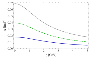
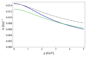
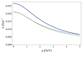
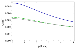
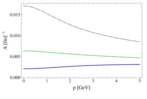
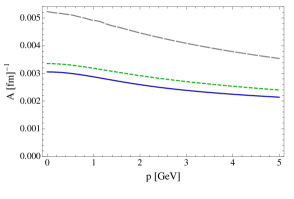
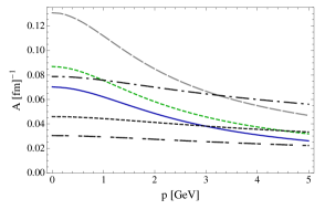
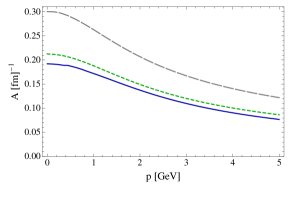
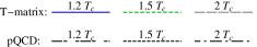
Figure 8: Friction coefficients in the $S$-wave (left) and $P$-wave (right) for charm-gluon scattering with potential $U$ in triplet (top), sextet (2nd row) and 15-plet (3rd row) color channels. The sum of all gluon contributions is displayed at the bottom left while the total sum of gluons, light and strange quarks is at the bottom right. (Color online.)

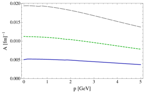
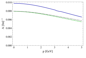
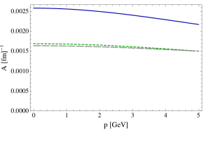
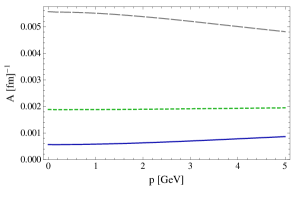
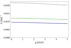
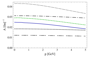
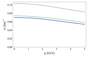
Figure 9: Same as Fig. 8, but for bottom quarks.

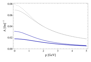
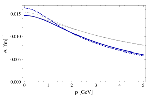
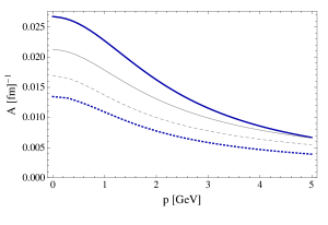
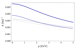
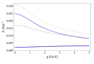
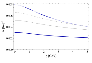
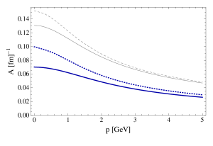
Figure 10: Drag coefficients calculated with only the Coulomb part of the in-medium $U$ potential (dashed/dotted lines), compared to the full potential (solid lines), for charm-gluon interactions at 1.2 $T_{c}$ (thick blue lines) and 2.0 $T_{c}$ (thin gray lines). (Color online.)

The lower right panel in Fig. 8 summarizes the total $c$-quark relaxation rates in a QGP with 2+1 flavors as obtained from our elastic in-medium $T$-matrices, by adding the here calculated gluon contributions to the $u$, $d$ and $s$ anti-/quark contributions calculated in Ref. Riek:2010fk (lower left panel of Fig. 23 in there). Not unexpectedly, replacing the perturbative gluon part in there with the nonperturbative $\tilde{T}$-matrix, the total drag coefficient increases by about 25% at low momenta (somewhat more at 1.2 $T_{c}$ and somewhat less at 2 $T_{c}$). However, at charm-quark momenta of about 5 GeV (and above), we find a slight decrease of the total $A$. The reason is that the perturbative gluon contribution in Ref. vanHees:2004gq ; Riek:2010fk has been calculated with $\alpha_{s}=0.4$, while the lQCD free-energy fits result in $\alpha_{s}\simeq 0.3$ for the Coulomb part (which dominates at high momenta). This reiterates that our calculations approach the leading-order pQCD limit at high momenta, i.e., the resummation effects cease. In particular, it demonstrates that the use of a schematic momentum-independent $K$-factor to upscale perturbative results in the low-momentum regime will lead to incorrect results at high momentum. A proper dynamic treatment of the nonperturbative effects is thus mandatory to obtain a realistic momentum dependence of the HQ transport coefficient in the QGP. In a sense, this is a reflection of the asymptotic freedom property of QCD, with a dynamical generation of nonperturbative effects in the low-energy domain. Again, similar considerations apply in the bottom sector, only that the momentum scale for recovering perturbative results is augmented relative to the charm case by roughly the mass ratio of $m_{b}/m_{c}\simeq 3$.

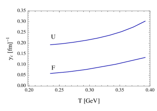
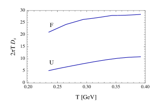
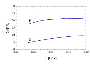
Figure 11: Charm (left) and bottom (right) relaxation rates (upper) and diffusion constants (lower) using $U$ and $F$ as a potential.

We also examine the drag coefficient computed from utilizing the Coulomb-only potential for charm-gluon interactions, cf. Fig. 10. First, all channels are subject to an overall kinematic effect due to the smaller in-medium charm-quark mass, by about 20(10)% at 1.2(2) $T_{c}$, which increases the thermal relaxation rate accordingly. Additional effects arise dynamically due to changes in the $\tilde{T}$ matrix and thus vary depending on the channel under consideration. In the color-$3$ $S$-wave, there is a moderate enhancement of the Coulomb-only over the full potential for 1.2 $T_{c}$ at small momenta which is partly due to the bound state (or resonance) being located closer to the 2-particle threshold owing to less binding in the absence of the string term; this provides more $\tilde{T}$-matrix strength in the scattering regime. At 2 $T_{c}$ this effect is no longer operative (the small enhancement is compatible with the kinematic effect alone). In the 15-plet, the enhancement of the Coulomb-only case over the full potential is more pronounced, especially at low temperature, due to the absence of the compensation between attractive string and repulsive Coulomb terms. In the sextet, on the other hand, one finds an overall suppression effect: despite the smaller $c$-quark mass, the large loss in near-threshold $\tilde{T}$-matrix strength due to the absence of the string term leads to a reduction of the relaxation rate. The total HQ relaxation rate from interactions with thermal gluons increases in the Coulomb-only case relative to the full calculations by $\sim$40(15)% at 1.2(2.0) $T_{c}$, i.e., the nonperturbative effect fades away toward higher temperatures, as expected. At 1.2 $T_{c}$, the suppression of the $S$-wave sextet (factor of 0.5) is more than compensated by a 70% increase in the triplet and the large enhancement of the 15-plet (factor of $\sim$10). At 2 $T_{c}$, the effects of the missing string term essentially compensate each other between the different channels, leaving a net increase of $\gamma_{c}$ which is close to the expected mass scaling. At high momenta, where both mass and nonperturbative effects are expected to become suppressed, we indeed observe a general tendency of convergence of the full and the Coulomb-only potential results.

We finally relate the relaxation rate at zero momentum to the spatial diffusion coefficients by

$$D_{s}=\frac{T}{m_{Q}\gamma_{Q}}\ .$$ (59)

Note that this quantity essentially divides out the kinematic “delay” of $\sim$$T/m_{Q}$ of the relaxation rate for a massive particle. Thus, in first approximation one may expect $D_{s}$ to be independent of the HQ mass. This is one of the main reasons why this quantity, after scaling by temperature to a dimensionless quantity, has been used as an indicator of a general transport parameter of the QCD medium, namely the ratio of viscosity to entropy-density, $\eta/s\simeq cTD_{s}$. The coefficient $c$ typically ranges from 1/5 to 1/2 in weakly and strongly coupled plasmas, respectively. In Fig. 11 we summarize the temperature dependence of $\gamma_{Q}$ (upper panels) and $D_{s}$ (lower panels) from our calculations for charm (left panels) and bottom quarks (right panels), using both free and internal energies for the input potentials. For the relaxation rate, we roughly find the expected mass scaling by a factor of $m_{c}/m_{b}$ when going from charm to bottom, for both $F$ and $U$ potentials. For charm quarks the difference between the potentials translates into a factor of 4(2.5) increase in the relaxation rate at low (high) temperatures. This is somewhat less pronounced for bottom. The anticipated independence of $D_{s}$ on mass holds well for the $U$ potential (within ca. 10%), while for the $F$ potential the deviations are somewhat larger (ca. 20-25%). If $TD_{s}$ is indeed proportional to $\eta/s$, all results are suggestive for a shallow minimum toward the critical temperature, which is nontrivial since it implies a marked increase in interaction strength with decreasing temperature. Quantitatively, our newly included nonperturbative treatment for HQ-gluon scattering reduces $D_{s}$ by about 25% relative to our previous results Riek:2010fk ; for the $U$-potential both charm and bottom give $TD_{s}\simeq 0.8$ at the lowest temperature, which would imply $\eta/s\simeq 0.16-0.4$.

VI Conclusion

In this paper we have extended a previous in-medium $T$-matrix approach for elastic heavy-quark scattering off light anti-/quarks in a deconfined plasma to the thermal gluon sector. Our main objective was the evaluation of relativistic corrections to the static potential and a reliable matching of normalization factors to account for the spin-1 properties of the gluons. We also investigated the possibility of thermal corrections to the gluonic vertices and restricted the gluon polarizations to the physical transverse ones in the presence of a thermal mass. The diagrammatic analysis of Coulomb and string contributions to the potential led to relativistic corrections paralleling the light-quark case. Upon a ladder resummation in the $T$-matrix equation, we found the emergence of HQ-gluon resonance structures in the attractive color-Coulomb channels close to the 2-particle threshold at QGP temperatures close to the critical one. The peak structures gradually dissolve with increasing temperature but an appreciable near-threshold enhancement persists even at 2 $T_{c}$. These nonperturbative effects in the scattering amplitudes lead to a marked enhancement of the pertinent transport coefficient (thermal relaxation rate), by up to a factor of 3 at low HQ momenta and close to $T_{c}$. At higher momenta, $p\gg m_{Q}$, the rates approach perturbative values, thus reiterating the importance of a dynamical treatment to consistently account for the momentum dependence of HQ transport in the QGP. We furthermore investigated the interplay of Coulomb and string terms; by switching off the latter, a nontrivial interplay between kinematic mass reduction, binding effects and the lack of constructive (destructive) interference in the attractive (repulsive) Coulomb channels was observed. These effects ceased with increasing temperature, signaling the fading of the string term.

By combining the nonperturbative gluon contribution with previous calculations in the light- and strange-quark sector we found that an overall enhancement of the low-momentum transport coefficient by about 25% emerges, while the high-momentum part is little affected (indicating even a slight decrease compared to the previous perturbative treatment with larger coupling). These updates should be included in phenomenological applications to heavy-quark observables at RHIC and LHC He:2012df . When coupled with a quantitatively constrained bulk evolution model (e.g., relativistic hydrodynamics), the updated input rates can serve as a rather complete baseline for the contribution of elastic interactions in the HQ diffusion process. We recall that at low momenta these are the only interactions contributing to the transport coefficient. When coupled with a realistic hadronization description and subsequent hadronic diffusion in a heavy-ion reaction, a detailed comparison with experiment can then reveal remaining shortcomings in the description, most notably contributions from radiative processes which are expected to become relevant at (much) higher HQ momenta. Work in these directions is in progress.

- (1) R. D. Pisarski, p. 353 (2002), arXiv:hep-ph/0203271.
- (2) O. Kaczmarek and F. Zantow, Phys. Rev. D 71, 114510 (2005).
- (3) P. Petreczky and K. Petrov, Phys. Rev. D 70, 054503 (Sep 2004).
- (4) K. Nakayama and W. G. Love, Phys. Rev. C 38, 51 (1988).
- (5) R. Rapp, H. van Hees, in R. C. Hwa, and X.-N. Wang (Ed.), Quark Gluon Plasma 4. p. 111 (2010).
- (6) F. Riek and R. Rapp, Phys. Rev. C 82, 035201 (2010).
- (7) H. van Hees, M. Mannarelli, V. Greco, and R. Rapp, Phys. Rev. Lett. 100, 192301 (2008).
- (8) D. Cabrera and R. Rapp, Phys. Rev. D 76, 114506 (2007).
- (9) M. Mannarelli and R. Rapp, Phys. Rev. C 72, 064905 (2005).
- (10) A. Bazavov, P. Petreczky, and A. Velytsky, (2009), arXiv:0904.1748 [hep-ph].
- (11) E. Megias, E. Ruiz Arriola, and L. Salcedo, Phys. Rev. D 75, 105019 (2007).
- (12) E. Megias, E. Ruiz Arriola, and L. Salcedo, JHEP 0601, 073 (2006).
- (13) O. Kaczmarek, PoS CPOD07, 043 (2007).
- (14) E. V. Shuryak and I. Zahed, Phys. Rev. D 70, 054507 (2004).
- (15) J. Bjorken and S. Drell, Relativistic Quantum Mechanics, International series in pure and applied physics (McGraw-Hill, New York, 1964).
- (16) M. Goldberger and K. Watson, Collision Theory, Dover books on physics (Dover Publications, New York, 2004).
- (17) V. Herrmann and K. Nakayama, Phys. Rev. C 46, 2199 (1992).
- (18) E. Braaten and R. D. Pisarski, Nuclear Physics B 337, 569 (1990).
- (19) E. Braaten and R. D. Pisarski, Nuclear Physics B 339, 310 (1990).
- (20) R. Mertig, M. Böhm, and A. Denner, Computer Physics Communications 64, 345 (1991).
- (21) P. Lévai and U. Heinz, Phys. Rev. C 57, 1879 (1998).
- (22) M. Cheng, N. Christ, S. Datta, J. van der Heide, C. Jung, et al., Phys. Rev. D 77, 014511 (2008).
- (23) E. E. Salpeter and H. A. Bethe, Phys. Rev. 84, 1232 (1951).
- (24) R. Machleidt, Adv. Nucl. Phys. 19, 189 (1989).
- (25) R. Thompson, Phys. Rev. D 1, 110 (1970).
- (26) R. Woloshyn and A. Jackson, Nucl. Phys. B 64, 269 (1973).
- (27) M. Bellac, Thermal Field Theory, Cambridge Monographs on Mathematical Physics (Cambridge University Press, Cambridge, 2000).
- (28) M. Cheng, S. Ejiri, P. Hegde, et al., Phys. Rev. D 81, 054504 (Mar 2010).
- (29) F. Riek and R. Rapp, New J. Phys. 13, 045007 (2011).
- (30) B. Svetitsky, Phys. Rev. D 37, 2484 (1988).
- (31) H. van Hees and R. Rapp, Phys. Rev. C 71, 034907 (2005).
- (32) M. He, R. J. Fries, and R. Rapp, (2012), arXiv:1204.4442 [nucl-th].